Fatbox: the Fault Analysis Toolbox

Analysing the spatial arrangement, connectivity, and evolutionary history of complex fault networks is essential for quantifying strain distribution in active deformational zones, and evaluating associated geohazard and resource potentials. The structure and evolution of fault networks are commonly investigated using a range of methods, including the analysis of topographic data derived from satellite imagery, numerical modelling, as well as physical experiments. The high density and intrinsic complexity of fault systems in many study areas or models pose significant challenges for automated analysis, often necessitating time-intensive manual interpretation. Here, we present Fatbox, the Fault Analysis Toolbox, an open-source Python library that integrates semi-automated fault extraction with automated geometric and kinematic analysis of fault networks. The toolbox capabilities are demonstrated through three case studies on normal fault systems, each drawing on a different data type: (1) fault extraction and geometric characterization using GLO-30 topographic data in the Magadi-Natron basin in East Africa; (2) spatio-temporal tracking of fault development in vertical cross-sections of a forward numerical rift model; and (3) surface fault mapping and geometric evolution of a physical rifting experiment. Fatbox represents fault networks as topological graphs, comprising nodes (i.e., points) and edges (i.e., lines) connecting the nodes. In time-dependent models, the toolbox enables temporal tracking of faults, providing detailed insights into their geometric evolution and facilitating high-resolution measurements of fault kinematics. Fatbox offers a versatile and scalable framework that enhances the efficiency, reproducibility, and precision of fault system analysis – opening new avenues for tectonic research.

1 Introduction

Faults accommodate shear displacements and form when applied stresses exceed the mechanical strength of the host rock. These structures occur across a vast range of spatial (from micrometres to kilometres) and temporal (from years to millennia) scales (Scholz, 2019), often evolving into intricate, highly complex networks (Osagiede et al., 2023; Tewksbury et al., 2014). This complexity reflects the evolution of fault architecture over time as individual faults grow, interact, and sometimes link together (Faulkner et al., 2010; Rotevatn et al., 2019),. This growth and interaction process plays a crucial role in shaping the fault network's geometry and mechanical behaviour. Geometric analyses of fault structures can therefore be used to estimate regional strain and, where sufficient temporal constraints exist, to quantify strain rates – analyses that are mostly conducted in continental rifts where normal fault networks are identifiably from satellite data (La Rosa et al., 2025; Polun et al., 2018; Riedl et al., 2022). At plate boundaries, faults are fundamental in accommodating strain, and detailed characterization is essential for evaluating the contribution of distributed, off-fault deformation to the total slip budget (Herbert et al., 2014). Beyond their mechanical role, faults significantly influence the rheological and transport properties of the crust by serving as conduits for fluids, volatiles, and deeply sourced gases (Frondini et al., 2008; Muirhead et al., 2020; Tamburello et al., 2018). In continental rifts, fault activity is frequently happening in alternance with magmatic processes, and serves as a key control on the structure of geothermal systems located above magmatic systems (Corti, 2012; Jolie et al., 2021). (Faulkner et al., 2010; Rotevatn et al., 2019).

Fault networks can be investigated using a range of complementary techniques, each offering a different perspective on deformation processes:

1. Mapping of natural fault systems combines various field, remote sensing and geophysical methods to identify and characterize faults at the surface and at depth. Geological mapping focuses on the surface expression of faults (Muirhead et al., 2016), while seismic data helps detect subsurface displacements along stratigraphic horizons (Wrona et al., 2023). Magnetotelluric surveys further contribute by mapping variations in electrical resistivity, which can indicate the presence of fluids or fault zones at depth (Martí et al., 2020), and can be used in conjunction with satellite imagery. Normal faults, in particular, are well-suited for remote sensing approaches due to their strong topographic signature in extensional settings. These faults can be detected either by identifying topographic shifts caused by displacement – using resources such as the Copernicus GLO-30 dataset, an open-source global topographic model released by the European Space Agency in 2019 – or by recognizing their traces in optical imagery (La Rosa et al., 2022). Unlike thrust faults within contractional settings where the hanging wall collapse and obscures the fault scarp, normal faults produce first-order topographic features that make them especially visible in satellite data.

2. Numerical modelling provides a powerful tool for simulating geodynamic processes over spatial and temporal scales relevant to Earth's evolution. These models incorporate well-constrained rheological properties of Earth's layers (Bürgmann and Dresen, 2008), simulating deformation through brittle failure (Davis and Selvadurai, 2002) or ductile flow based on experimentally-derived flow laws (Hirth and Kohlstedt, 2004). Depending on the research focus, models may address fault evolution in crustal-scale setups (Allken et al., 2011) or include the mantle to examine long-term rift evolution and the onset of seafloor spreading in extensional systems (Li et al., 2024). Although often conducted in two dimensions, such simulations offer high spatial resolution, enabling detailed exploration of fault geometries and their temporal development (Neuharth et al., 2022).

3. Laboratory-based physical experiments are conducted to simulate natural geological processes, employing a variety of experimental configurations designed to accurately replicate the key elements of the target system. In the study of normal fault systems, analogue modelers commonly utilize table-top experiments, wherein the mechanical properties and physical dimensions of the model materials are scaled to represent those of the crust (Maestrelli et al., 2024; Zwaan et al., 2021). Topographic changes are systematically monitored throughout the experiment using digital cameras, enabling the reconstruction of surface morphology at regular time intervals and the optical tracking of fault network evolution. The acquired image sequences are subsequently processed using Particle Image Velocimetry (PIV), which allows for the calculation of velocity fields and the generation of strain maps, thereby quantifying the kinematic development of the physical model (Strak and Schellart, 2016).

Natural fault and fracture systems are commonly mapped using field, satellite, and geophysical data (Claringbould et al., 2020; Muirhead et al., 2016) and manual faults interpretations performed by expert geologists and corroborated by field observations are the most common and reliable methods (La Rosa et al., 2022; Muirhead et al., 2016). However, this approach demands substantial expertise and time, and mapping consistency is not always ensured, especially in large areas (Bond, 2015). Semi-automated workflows can perform high-resolution fault mapping using regional DEMs (Ahmadi and Pekkan, 2021), though these methods necessitate careful calibration against manual interpretations to ensure accuracy. Recently, several semi-automated fault detection methods have been (Healy et al., 2017; Wrona et al., 2021; Zielke et al., 2010). Certain approaches focus on the quantification of lateral and vertical displacements by analysing geomorphological offsets, such as river channel shifts (Stewart et al., 2018; Zielke et al., 2012). Other methods employ U-Net convolutional neural networks for the automatic detection of fractures and faults in optical images and DEMs (Mattéo et al., 2021). Existing tools are typically designed for a specific task, such as network extraction from images (Dirnberger et al., 2015), topological analysis (NetworkGT by Nyberg et al., 2018), remote sensing data processing (Ahmadi and Pekkan, 2021), fracture system analysis (FracPaq by Healy et al., 2017), or automated throw calculation (e.g. ScarpLearn by Pousse-Beltran et al., 2025; Auto_Throw by Giampietro et al., 2025). However, so far, no tool unites these functionalities within an open-source framework that allows multiple data source types, temporal correlation, and both geometric and kinematic fault descriptions.

Here we introduce Fatbox – the Fault Analysis Toolbox, an open-source Python software that includes a comprehensive suite of functions for extracting and analysing faults and fractures in various observational datasets and models. In Fatbox, faults are described as networks that capture the spatial evolution of the systems, which allows for the representation of rich and complex geometries as observed in natural fault networks. Additionally, the toolbox includes functions for correlating faults over time, allowing for the tracking of the system's temporal evolution. Furthermore, classical geometric fault analysis parameters like length, throw, and displacement (Fossen, 2016) have been incorporated to quantify and visualize fault network evolution. In this study, we focus on extensional settings to present the different functionalities of Fatbox using three application examples that best illustrate its potential: (1) mapping and geometric analysis using a topographic dataset from the Magadi-Natron basin, (2) extracting and tracking fault evolution in depth profiles using strain rate data from a numerical rift model, (3) monitoring topography and incremental strain evolution in a physical extension experiment. Each application serves to illustrate specific functionalities of the toolbox, addressing distinct analytical requirements. While our examples focus on extensional settings, the underlying tools are designed to be flexible and broadly applicable.

2 Background and technical setup

2.1 Definitions and graph description

Fatbox extracts and quantifies the geometry of fault networks, accounting for their complex spatial and temporal evolution. Developed in Python 3.9, Fatbox provides functions for mapping, editing, analysing, and tracking the temporal evolution of fault networks. Two types of input data are typically used: topography or strain. The fault extraction can be conducted semi-automatically or imported in the workflow from an existing dataset of manually picked faults.

In Fatbox, we represent fault systems as topological networks. Each extracted fault is defined as a component of the larger network and assigned a unique identification number, or label. These components are organized within a graph object (NetworkX, Hagberg et al., 2008), a structure that is similar to a dictionary and that allows manipulating the graph components and their associated attributes. Each network component comprises nodes (points defined by their x and y coordinates) and edges (connections between nodes) (Fig. 1B–D). We compute and store attributes for each element, such as the strike of an edge or the length of a component, allowing rapid and straightforward data access. This network-based framework effectively captures the connectivity observed in natural fault systems, including features such as fault splays (nodes with three connecting edges) and intersections (nodes with four connecting edges) (Fig. 1C–D). The key functionalities of the toolbox are (1) automated fault extraction from various datasets, including top-view and depth sections; (2) temporal tracking of structures; (3) quantification of multiple structural and geometric parameters across the fault network. Fault networks can be exported in raster, shapefile, and KMZ formats.

Fatbox comprises six Python module files and three Jupyter notebook tutorials. The modules organize the functions by specific tasks and are callable within separate scripts. The tutorials illustrate the main applications of the toolbox as detailed in this study: elevation data of a natural rift, numerical modelling, and analogue modelling. Each tutorial contains multiple Jupyter notebooks that outline key functionality step-by-step and explains the corresponding workflows. The figures accompanying the applications in this paper are generated using Fatbox tutorials and open-source data and results, ensuring reproducibility and providing users with easy access to the workflow. The toolbox is further supplemented on the GitHub repository with a glossary and a comprehensive documentation.

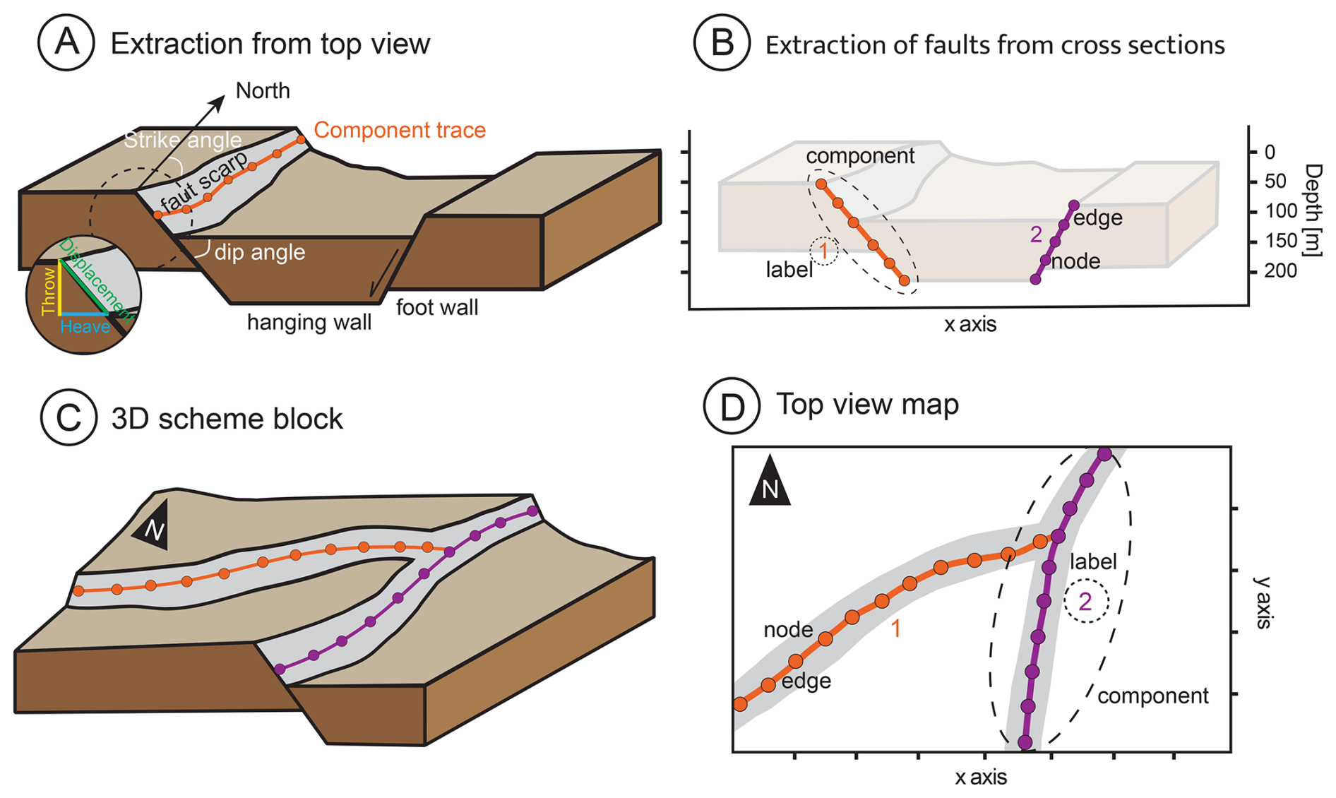
Figure 1 Network description exemplified using normal faults. The fault systems are described as networks, consisting of sets of nodes (depicted as circles in the figure) and edges (the segments connecting the nodes). The nodes are defined by their spatial (x, y) coordinates in 2D space, and the edges are defined as a pair of connected nodes. Components are groups of linked nodes; they represent individual faults. Per default, components are labelled via consecutive, integer fault identifiers. (A) Map view showing the location of the mapped faults on the scarp. Each fault is characterized by key geometric parameters: throw (vertical offset), heave (horizontal offset), and displacement (net slip). (B) Fault traces on a vertical cross section. (C) Triple junctions (or y-nodes) are split based on their orientation, ensuring that the two closest branches remain connected while the splay is cut off. (D) Top view of triple junctions illustrating the geometric configuration.

2.2 Accessibility and structure of the toolbox

The Fatbox repository is available on Github https://github.com/PaulineGayrin/Fatbox (last access: 25 February 2026).

Fatbox functions are grouped in 6 different Python scripts that follow a typical sequential workflow.

The 6 scripts of the library are accessible on Github in the folder /modules.

1. preprocessing.py. Prepare the dataset for fault network extraction.

2. edits.py. Extract the fault network from the dataset and edit the network structure and geometry, and its sub-networks.

3. metrics.py. Compute various metrics of the fault network, such as length of the edges, node properties, number of components.

4. plots.py. Visualize the fault network and results of the analysis.

5. utils.py. Various low-level helper functions.

6. structural_analysis.py. Measure the geometric properties of the faults.

The data and workflows demonstrated in this study are available in the folder /tutorials. The tutorials are designed to demonstrate the possibilities and explain key steps of the process.

2.3 Parameters, filters, recommendations

This library is implemented in a modular way to provide users with a high degree of control over the fault analysis process. Recognizing that each geological context and analytical application is unique, we intentionally minimize excessive automation and instead provide a few key parameters and filtering options. Users can perform fault extraction directly within the toolbox or import pre-existing fault mappings, which may be derived from established databases or field surveys.

In numerical continuum models, active faults are most efficiently identified using strain rate data (Duclaux et al., 2020; Jourdon et al., 2025; Naliboff et al., 2020; Pan et al., 2022). To separate fault networks from background deformation, thresholding settings are critical. Accordingly, several thresholding filters are available, each suited to different strain rate distributions: (1) Absolute thresholding (e.g., 10¹³ s⁻¹) performs optimally when strain rates vary little across timesteps. (2) Relative thresholding (e.g., a threshold at 90 % of the model's maximum strain rate) proves effective if absolute values fluctuate significantly between timesteps. (3) Adaptive thresholding (e.g., 90 % of the maximum strain rate within a moving window) is particularly suitable for highly heterogeneous strain rate that vary over time. In addition, faults can also be identified using accumulated strain (Neuharth et al., 2022), for which all of the aforementioned thresholding filters are equally available.

Topographic datasets often include a wide range of features that may be misidentified as faults by automated algorithms. It is therefore essential to apply wavelength-dependent filtering techniques to distinguish genuine fault-related structures from background noise. An initial step may involve smoothing the terrain using a Gaussian filter, although alternative smoothing techniques may also be applied. Faults are identified using the Canny edge detection algorithm, which incorporates secondary Gaussian smoothing. We recommend applying a stronger smoothing filter initially, followed by a more moderate filter during Canny edge detection. This approach often requires refinement by try and error to preserve structural features while minimizing noise, ideally retaining small-scale details without introducing excessive artefacts. In the final step, shapes smaller than a user-defined size threshold can be removed to reduce residual noise. We advise using this filter moderately to avoid over-filtering and losing meaningful geological features.

The quality of fault mapping from topographical data is enhanced through the synergistic application of multiple filters, rather than reliance on a single dominant filter. Within a given dataset, noise typically exhibits distinctive characteristics – often manifesting as small, curved artefacts. The toolbox provides a range of functions designed to refine noisy fault networks, based on length (e.g., remove_small_object, remove_small_components), curvature (e.g., remove_cycles, cut_U_bend_curvature), and connectivity (e.g., remove_node_alone, remove_self_edge). We recommend to visually inspect the fault network and visually distinguish between actual faults and artefacts, and to select the most appropriate filters accordingly.

Automated quantification of fault geometry from topographic data is part of the structural analysis step and requires only a single user-defined parameter: the distance d (given in pixels). The fault scarp geometry is extracted along a line perpendicular to the fault strike. The algorithm identifies the up-dip and down-dip ends of the scarp within a window extending a distance d on either side of the mapped fault trace. Once the scarp's elevation profile is extracted, its length and both horizontal and vertical extent are stored. In the current methodology, d is applied uniformly across the entire dataset. To determine an optimal value for d, users should consider the average inter-fault spacing within the dataset: d must be sufficiently small to exclude adjacent faults from the profile yet large enough to capture the full extent of the scarp.

3 Applications

In order to demonstrate the capabilities of Fatbox, we present three different applications addressing typical challenges: (1) fault extraction and geometric analysis from topographic data of the Magadi-Natron basin in the East African Rift; (2) fault extraction and temporal correlation from strain data in a numerical rift model; (3) geometric evolution of faults based on topography and strain data of an analogue rift model.

3.1 Application 1: Topography-based fault analysis in the Magadi-Natron basin, East Africa

Digital Elevation Models (DEMs) represent normal faults at the surface as abrupt changes in altitude (Muirhead et al., 2016). Remote sensing captures elevation, vegetation, and anthropogenic features, enabling identification and reconstruction of the ground surface in digital surface models, which we will refer to as DEMs for convenience. In geological studies, DEMs are a valuable tool for analysing the structural framework and kinematics of tectonically active regions (Panza et al., 2024). Arid regions, due to their low erosion rates, frequently exhibit well-preserved fault scarps, which facilitate the accurate measurement of fault geometries. For fault network analysis, the broad range of DEM resolutions enables detailed investigations of small areas (tens of kilometres) with a high density of detected faults, as well as regional-scale studies (hundreds of kilometres) where only major faults are identified. In 2019, the European Space Agency released GLO-30, an open-source global DEM with a 30 m resolution (Copernicus ESA, 2019, https://doi.org/10.5270/ESA-c5d3d65). GLO-30 provides a high-quality landscape representation based on commercial data from TanDEM-X SAR satellites (Purinton and Bookhagen, 2021). Accordingly, our study utilizes GLO-30 to leverage freely available data while maintaining high-resolution quality.

3.1.1 The Magadi-Natron basin

The East African Rift System (EARS) is the largest active continental rift on Earth and exhibits tens of thousands of normal faults that displace the surface sufficiently to be recognized in satellite-derived digital elevation models (Fig. 2). In the following example, we apply Fatbox to the Magadi-Natron basin, which is located in the Eastern Branch of the EARS in Kenya and Tanzania. The borders of the basin are limited by mature normal faults. The intra-rift region was buried beneath a layer of Magadi trachyte approximately 1.2 million years ago (Baker and Wohlenberg, 1971; Muirhead et al., 2016). These lava flows have reset most of the basin's topography, meaning that the normal fault scarps in the Magadi-Natron basin are no older than 1.2 million years. In addition, the fault scarps are well preserved (Riedl et al., 2020) thanks to the arid environment, sparse vegetation and hence low erosion rate. The basin features a dense and complex fault network with minimal cross-cutting structures, making it an ideal case study. To illustrate our workflow, we apply Fatbox to a 175 km² area covered by the DEM, accurately representing the natural complexity of the region.

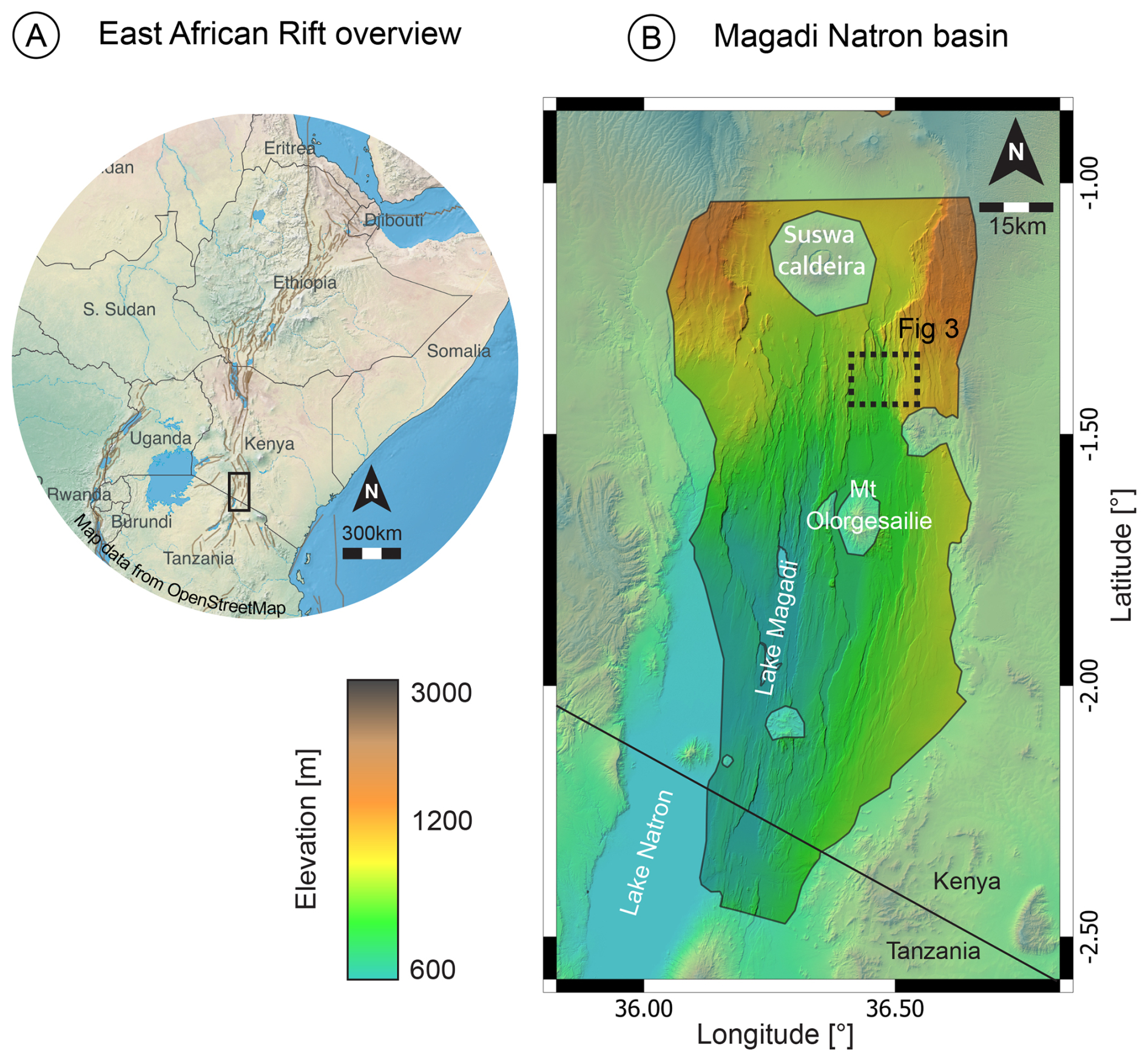
Figure 2 Context map of the DEM application. The Magadi-Natron basin is located south of the magma-rich eastern branch of the East African Rift System. (A) the major active faults are drawn in brown, from Styron and Pagani, 2020, on OpenStreetMap contributors 2025. Distributed under the Open Data Commons Open Database License (ODbL) v1.0. (B) the colours represent the topography using GLO-30 DEM. The blue shaded background represents the clipping mask used to focus on the intra-rift faults. The black dashed frame is the small area used in Fig. 3 and in the DEM tutorial.

3.1.2 Fault extraction from topography

We illustrate the extraction of fault networks from topography using the DEM GLO-30 of the Magadi-Natron basin as input (Fig. 3A). First, a Gaussian blurring filter is applied to smooth small-scale ground variations that do not constitute significant structural signals. This approach enhances the signal-to-noise ratio of fault scarps. The edges of the scarp are then detected using the Canny edge detection algorithm (Canny, 1986). This process employs the first derivative of a Gaussian filter to compute the magnitude of topographic variations. A subsequent threshold filter isolates the pixels corresponding to identified edges, yielding an outline of topographic features. However, this method may also highlight additional structures, including river banks, volcanic edifices, and lava flows. These non-fault-related components exhibit distinct geometric signatures and are subsequently filtered out by using dedicated functions (available in the library) based on curvature and length. Next, the edges of the detected structures are reduced to one-pixel wide lines through skeletonization using the thinning algorithm of Guo and Hall (1992) (Fig. 3B). Other types of skeletonization techniques are described in Sect. 3.2.2 and can be used per user decision. Finally, a connection detection function identifies adjacent pixels as connected components, assigning the same component identifier to pixels belonging to a continuous fault trace. Each pixel within the detected structures is transformed into a node, while the edges of the network establish connections between these nodes (Fig. 1D), effectively completing the network extraction process (Fig. 3C). To avoid too dense node densities that impede performance, a filtering function is applied to selectively remove nodes at regular intervals. This approach optimizes computational efficiency while preserving a reasonable resolution.

As an alternative option to automated fault detection, a fault network can also be imported from previous manual mapping. This allows the user to assess the quality of the semi-automated mapping against established and trusted datasets. Manually mapped faults can be directly imported as geotiff. The fault traces are categorized as single structures in the connection detection step and the raster is then transformed into a network, analogous to the automated mapping process.

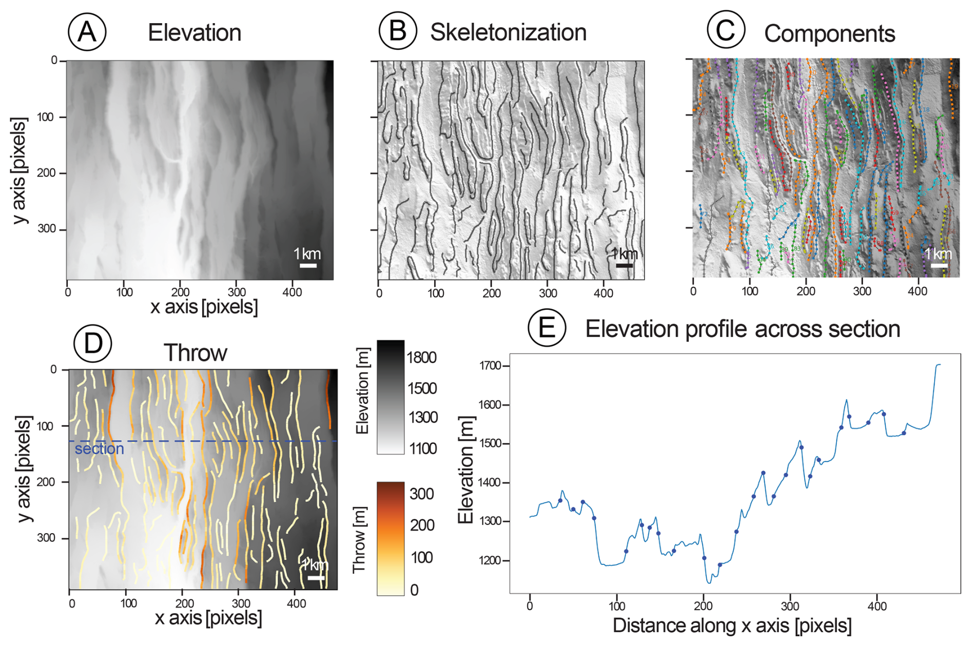
Figure 3 Workflow of the DEM processing. (A) Raw digital elevation model, (B) Skeleton, detected structures are 1 pixel wide, plotted over a hillshade of the DEM. (C) Fault network over DEM and hillshade of DEM. Different colours represent different components. (D) Throw over DEM. (E) E–W cross section perpendicular to the main fault axis at latitude 1.37° S, location shown in panel (D). The dots represent the position of the mapped faults.

3.1.3 Structural analysis

The surface expression of faults contains a wealth of structural information, which is critical for geological interpretation. Through fault extraction, the centre of the fault scarp along each fault trace is accurately determined (Fig. 1A). Subsequently, Fatbox conducts a systematic and automated structural measurement for each edge along the identified faults. This process replicates field-based procedures where geologists traverse fault lines and measure scarp geometry at regular intervals. Ultimately, diverse geometrical attributes are measured (Fig. 1A). The along-strike length of a fault is computed by summing the lengths of the edges belonging to the component, extending from one fault tip to the other. The azimuth (strike angle) is determined for each fault component. To determine the scarp geometry, a virtual cross section is drawn perpendicular to the fault axis until reaching a predefined maximum distance d (Sect. 2.3). During the structural analysis of the fault scarp, we derive fault displacement (net slip), extension (heave), and the fault's vertical offset (throw). These geometric attributes are assigned to the edges of each fault network component, which function as an independent data structure. This organization allows for direct access to the geometric properties of entire fault components. Within each component, nodes retain their spatial coordinates and the number of neighbouring connections, while edges store attributes such as length, connected nodes, strike, extension, and net slip. This structured framework ensures that all geometric information is stored comprehensively and remains readily accessible for further analysis.

Although the Magadi-Natron basin is a relatively arid region, erosion affects fault scarp morphology over long geological time scales. Erosional processes remove material from the footwall, rounding the initially sharp fault scarp, while deposition occurs onto the hanging wall, partially infilling the bottom of the fault surface. To mitigate these effects, throw measurements are taken at a reasonable distance from the fault crest, and a 60° fault dip is assumed for extension calculations (Fossen, 2016; Riedl et al., 2022). This dip angle is consistent with previous displacement-length studies in the Kenya Rift (e.g., 60° in Muirhead et al., 2016; 65° in Shmela et al., 2021). Additionally, apparent fault dip measurements can provide insights into the extent of erosion in a given area. As all the geometric attributes are stored for every edge, statistical analyses can be conducted on groups of faults based on criteria such as azimuth orientation and displacement. This facilitates comparative studies between faults or among different fault families. Furthermore, integrating the fault network with digitized geological maps enables comparisons between faults of similar maximum ages. Ultimately, structural analysis provides a comprehensive and quantitative characterization of fault surface expressions of the area.

3.2 Application 2: Fault tracking in numerical models

Numerical forward models have become a key approach in geodynamics where they are used to study a variety of processes across a broad range of scales, from large-scale mantle convection (Coltice et al., 2018) to subduction (Pons et al., 2022), rifting (Jourdon et al., 2020) and strike-slip tectonics (Heckenbach et al., 2024). Recent advances in computational techniques have allowed high-resolution 2D simulations yielding new insights into rift migration processes (Brune et al., 2014), deformation phases (Naliboff et al., 2017), and fault-related unconformities (Pérez-Gussinyé et al., 2020). While numerical models provide valuable insights into the long-term evolution of fault systems, the conducted fault analysis is often performed qualitatively or limited to discrete snapshots for direct comparison with natural data. Additionally, because faults in continuum models are represented as finite-width brittle shear zones, extracting slip rates and other quantitative parameters characteristic of discrete natural faults remains challenging. Recent studies using 3D continental rifting simulations have focused on quantifying the evolving characteristics of evolving fault network characteristics (e.g., Duclaux et al., 2020; Naliboff et al., 2020; Pan et al., 2022, 2023). Fatbox builds on this work by offering a framework to quantitatively extract and track the structure and evolution of faults through time, facilitating more accurate comparisons between numerical models and natural geological systems.

3.2.1 Numerical model setup

To illustrate the functionality of tracking temporal fault evolution, we use a 2D continental rifting model (Neuharth et al., 2022) where the geodynamic code ASPECT (Bangerth et al., 2024; Gassmöller et al., 2018; Glerum et al., 2018; Heister et al., 2017; Kronbichler et al., 2012) has been coupled to the landscape evolution code FastScape (Braun and Willett, 2013; Yuan et al., 2019). This model simulates a continental rift while incorporating sedimentation and erosion processes. The model domain is 450 km wide and 200 km deep. Prescribed boundary conditions enforce 5 mm yr⁻¹ extensional velocities on each side, resulting in a total extension rate of 10 mm yr⁻¹, while inflow is prescribed at the bottom boundary to maintain volume conservation. The 120 km thick lithosphere consists of 20 km of wet quartzite upper crust, 15 km of wet anorthite lower crust and 85 km of dry olivine mantle lithosphere (Fig. 4A). Beneath the lithosphere lies a weak asthenospheric layer composed of wet olivine (Neuharth et al., 2022). Rifting is initiated by thickening the upper crust to 25 km at the model's centre, leading to an initially warm and weak rift centre that ultimately evolves into a symmetric rift. Fatbox is employed to extract the faults and track their geometric parameters throughout the entire rift evolution.

3.2.2 Fault extraction from strain data

In these numerical models, faults are interpreted as zones of high strain or strain rate (Fig. 4A). Here we employ a strain-based fault criterion that distinguishes areas belonging to faults via a user-defined threshold (Fig. 4B). The thresholding assigns a value of 1 to pixels representing faults (where strain exceeds the threshold) and 0 to background pixels (where strain is below the threshold). In the following, we use a relative threshold (Sect. 2.3) that has been manually adjusted for optimal results. We then apply a thinning algorithm to extract the skeleton of each shape, reducing fault zones to single-pixel-wide lines (Fig. 4C). Various skeletonization algorithms exist, differing in quality and speed (see the review of Saha et al., 2016). Here we use the efficient Guo and Hall algorithm (Guo and Hall, 1992). Once skeletonized, individual faults can be distinguished and classified separately by identifying neighbouring pixels as part of the same connected component (Fig. 1B). Finally, the fault network is generated from the labelled components by converting each pixel to a point and connecting neighbouring points (Fig. 4D). Our ASPECT model uses an adaptative mesh refinement with spatially variable resolution. We load this variable grid and interpolate it onto an evenly spaced grid of pixels before performing the fault analysis in Fatbox (Neuharth et al., 2022). The extracted network can be very dense, with a node at each pixel belonging to a fault and edges connecting them. This excessive density can lead to unnecessarily long computation times. We therefore remove internal nodes (based on user-defined parameters), reducing density while preserving realistic geometric orientations.

3.2.3 Time stepping, correlation, and structural analysis

The fault extraction is performed independently at each time step, meaning that components receive labels that likely vary between steps (Fig. 4D–E). In order to track the evolution of the network, however, each fault must retain a consistent label throughout the workflow. We therefore introduce a correlation step that ensures that the same fault is identified by the same label across all time steps. Correlation is complicated by the fact that faults can advect, grow, shrink, appear, disappear, merge, or split. To account for these changes, faults at consecutive time steps are compared. In the simplest case (Fig. 5), we compare each fault at time n with each fault at time n+1 (forward) and each fault at time n+1 with each fault at time n (backward). If needed, correlations can be made across more than two time steps dependent on the temporal resolution of the model and the complexity of the network evolution. Individual faults are compared by computing the similarity between faults of different time steps. To this aim, we calculate the distance between each node and all the nodes of the graph at the other timestep. The average distance of two faults defines their similarity: two faults are considered similar when the average inter-fault distance falls below a user-defined radius R (in pixel) (Fig. 5). Selecting an optimal value for R is essential for achieving accurate correlations, often requiring an iterative trial-and-error process. Once correlations are established, faults from the later time step are relabelled according to the corresponding faults from the previous time step. This approach ensures a continuity of fault labels while establishing a time-dependent fault record.

Once faults are correlated through time, the temporal evolution of the fault system can be analysed. The subsequent structural analysis is performed at every time step and the geometric data are stored for the entire fault network. This dataset enables the tracking of kinematic properties such as displacement over time, allowing for the study of individual fault growth as well as the development of the entire fault system.

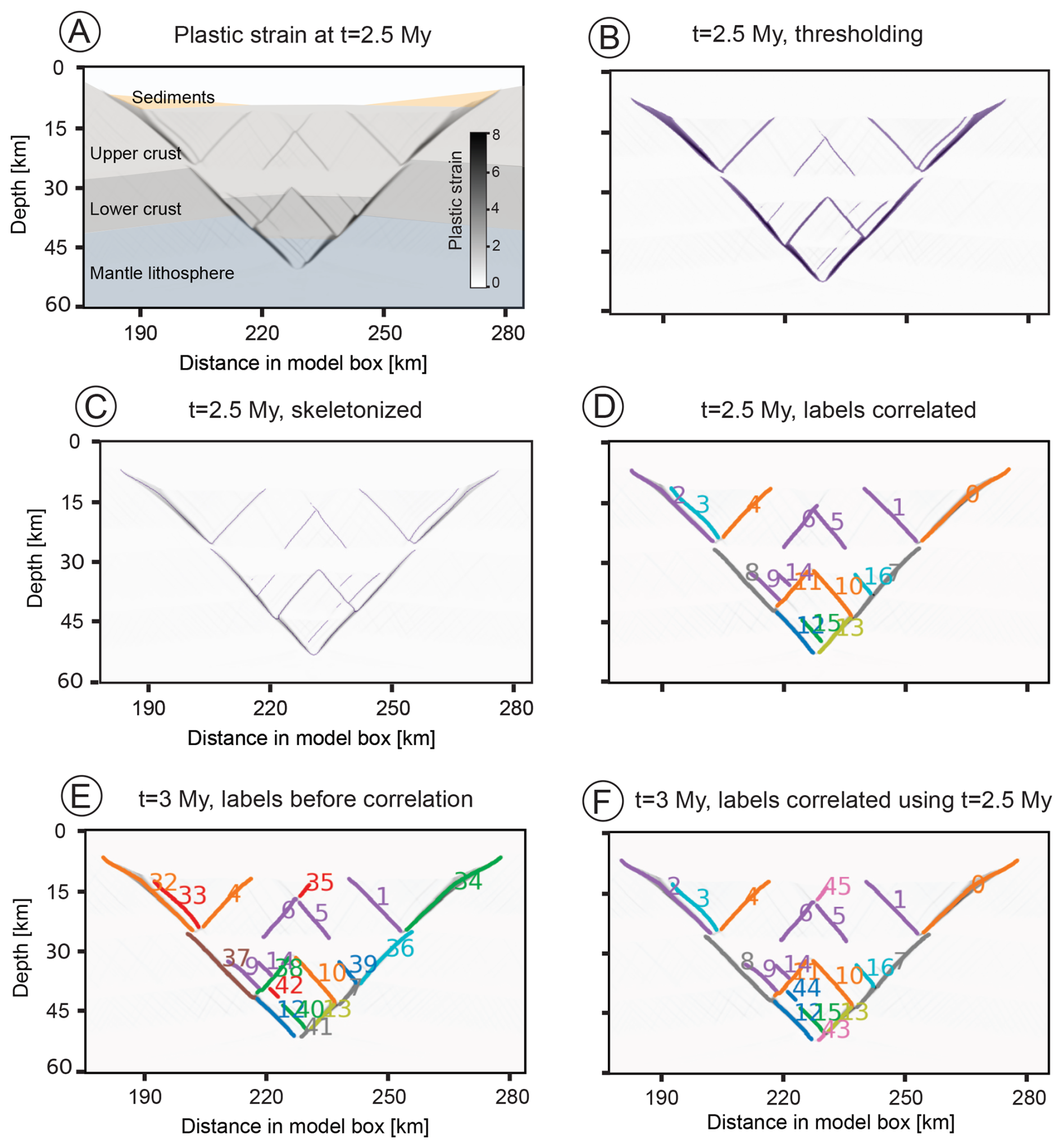
Figure 4 Fault correlation in a numerical rift model. (A) Material layers and plastic strain at t=2.5 Myr. The network consists of large border faults and smaller intra-rift faults. (B) Plastic strain at t=2.5 Myr, where pixels exceeding threshold strain are shaded in purple. (C) Skeletonization generates lines tracing the faults, here shown in purple underlain by plastic strain in grey scale. (D) Fault network extracted at t=2.5 Myr correlated using earlier and later time steps (forward + backward correlation). (E) Fault network extracted at t=3 Myr (before correlation). (F) Fault network at t=3 Myr, correlated using labels at 2.5 Myr. In practice, the period between subsequent correlation times is much smaller. This interval was chosen here to exhibit enough difference to show the effect of the correlation. The labels of the faults are shown as numbers next to the corresponding faults using the same colour.

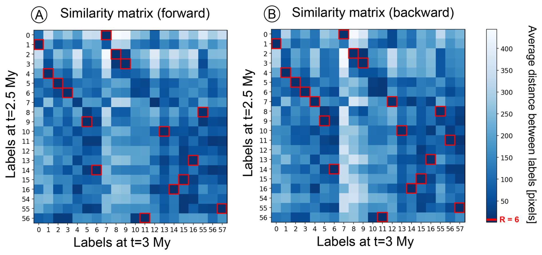
Figure 5 Correlation of faults across two time-steps. The similarity matrix shows all the labels of a pair of compared graphs. In (A), the forward direction means the graph at t=2.5 Myr is used as a base to compare with the graph at t=3 Myr. In backward direction (B), the base for the correlation is the graph at t=3 Myr. Faults with a low average distance exhibit a high similarity. The red squares indicate instances where the distance between two faults falls below a user-defined threshold radius R, representing the same fault at different times. Note that axes depict original labels that have not been correlated according to the full fault record.

3.3 Application 3: Topographic and incremental strain analysis of physical experiments

Analogue modelling is a key method in geodynamics, allowing researchers to replicate natural geological phenomena under controlled laboratory conditions with appropriately scaled lengths, times, and forces. Model evolution is usually monitored by digital cameras that record images at fixed intervals – every 10 min in the models used in this study. These images can be fed into Digital Image Correlation (DIC) analyses, which extract quantitative data from the visual record. Topographic data is derived from the digital images using photogrammetry techniques. When photogrammetry is unavailable, alternative methods such as laser scanning (Willingshofer and Sokoutis, 2009) or laser interferometry (Strak et al., 2011) are often. The Particle Image Velocimetry (PIV) technique calculates incremental displacement fields by cross-correlating digital images. This approach allows to detect texture patterns on the surface, sides, or interior of the model (Strak and Schellart, 2016).

Fault extraction is typically performed manually (Philippon et al., 2015; Schlagenhauf et al., 2008), a process that proves both very time-consuming and labor-intensive. To address these challenges, researchers have developed automated techniques to detect faults that utilize incremental strain maps derived from Particle Image Velocimetry (PIV). Some studies apply a global strain threshold to identify active strike-slip faults (Hatem et al., 2017; Visage et al., 2023) while others employ adaptive thresholds for more refined fault detection (Chaipornkaew et al., 2022; Gabriel et al., 2025). Here, we re-examine data from a study on rift propagation within a brittle-ductile multilayer physical experiment (Molnar et al., 2017). We use Fatbox to extract faults from both topographic and strain maps and secondly to combine time-tracking of faults and structural analysis of the topography.

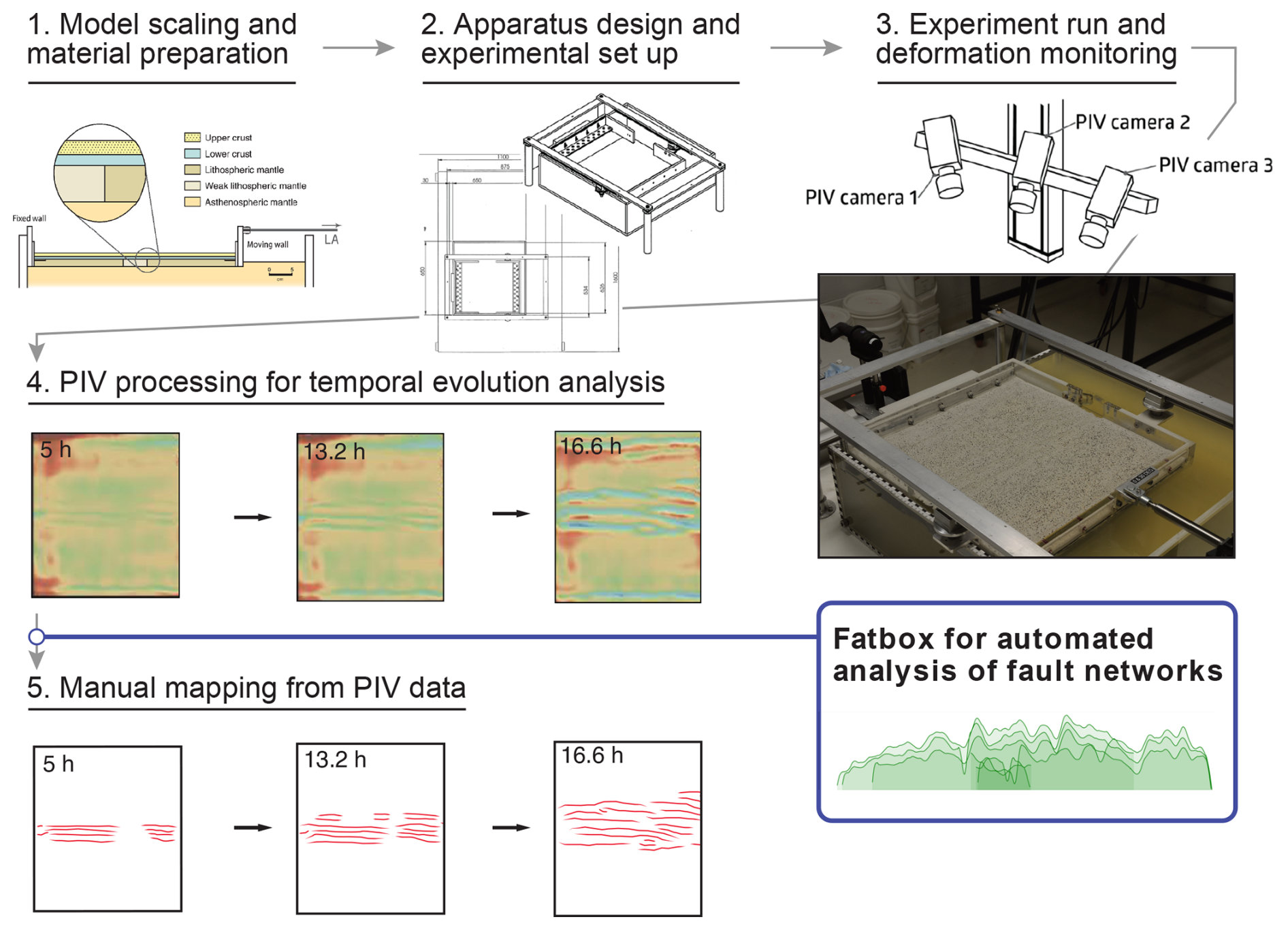
Figure 6 Integration of Fatbox in an analogue modelling workflow. The program replaces manual mapping and automatically analyzes the fault geometry and network evolution.

3.3.1 Fault extraction from elevation data

The digital photographs are captured at predefined time intervals, and the surface topography data is subsequently calculated. The fault extraction workflow is similar to the processing of DEM data (see Sect. 3.1.2) from satellite imagery. First, a Gaussian blur filter is applied to mitigate noise with a carefully chosen smoothing window, preserving the integrity of structural features. The background noise of analogue models is usually low and requires minimal smoothing. Feature edges are then detected using the Canny algorithm (Canny, 1986), which identifies intensity gradients in the images – serving as proxies for fault scarps. To transform these detected edges into lines, skeletonization is performed, refining the extracted lines to a one-pixel width. A connection detection function then identifies adjacent pixels as connected components, assigning the same component ID to pixels belonging to a continuous fault trace. Each pixel within the detected structures is transformed into a node, and the edges are generated to connect nodes based on their proximity, allowing faults to be clustered and labelled. Since this process may also detect non-fault features or artefacts, a final cleaning step is applied, considering attributes such as fault length, shape, and curvature. These operations are performed across all time increments in the dataset. Finally, all time steps are correlated to maintain the consistency of the labels (see Sect. 3.2.3).

3.3.2 Fault extraction and structural analysis from incremental strain data

Surface strain is computed by comparing one set of images with the subsequent set, providing values for incremental strain. Although this example applies the workflow to top-view images, it can also be adapted for side-view images of laboratory experiments. Faults are highlighted relative to the background using an absolute strain threshold that binarize the data (1 for fault and 0 for background). The subsequent workflow is the same as for the numerical model: structures are thinned to a single pixel width during the skeletonization (Guo and Hall, 1992). The connections are detected with each pixel being assigned the same component ID as its neighbouring pixels. The pixels are then converted into a node, and the collection of connection edges for each time increment is transformed into a network. Depending on the pre-processing stage (strain computation and data export), incremental strain datasets may contain varying levels of noise, heterogeneities, or areas with missing values. These issues can result in the incorrect identification of artefacts as faults, as in DEM application, see Sect. 3.1.2. An additional cleaning step is introduced to address this problem, which includes: (1) removing nodes connected to three or more other nodes, (2) slicing fault traces into smaller segments by eliminating nodes where the direction of the line edges deviates significantly (<120°) from neighbouring edges, and (3) removing components smaller than a defined length threshold. After cleaning the network, the final step is to correlate the faults across all time increments in the experiment dataset (Fig. 7A). When both incremental strain and elevation data are available, it is advisable to perform fault extraction on both datasets, compare the results, and use the one that yields better outcomes based on the available data.

The structural analysis is conducted as outlined in Sect. 3.1.3 for each time step. Here, the measured dip can be directly used to compute the displacement (net slip) and extension (heave) of the faults as erosion is absent. The correlation and proper labelling of faults between consecutive time steps enable the visualization of the evolution of specific geometric parameters over time. For example, the throw as a function of fault length (Fig. 7B) is commonly used to infer kinematics of normal fault growth (Lathrop et al., 2022; Schlagenhauf et al., 2008) and to assess the growth stage of the fault network.

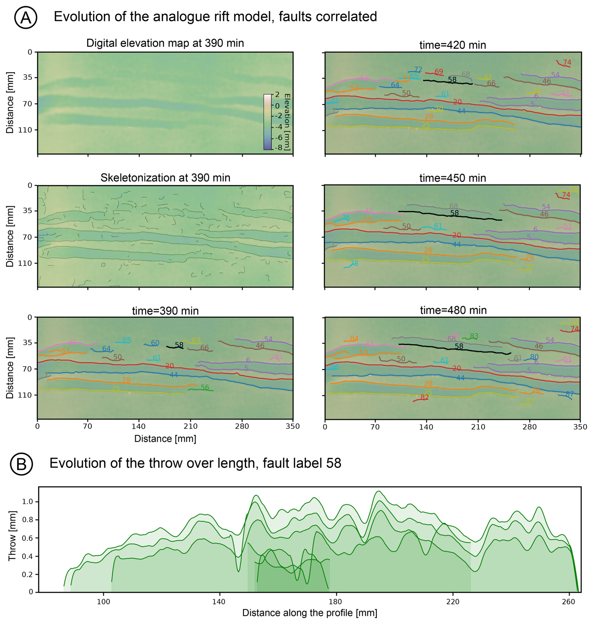
Figure 7 Temporal fault tracking in analogue models. (A) Evolution of the network during extension. The faults are correlated and tracked through time. (B) Throw length profile of the fault label 58. This ID is highlighted on (A) in black.

4 Discussion

4.1 Fatbox options for defining faults and describing fault networks

Fault extraction requires a clear criterion for fault identification, carefully adapted to both the dataset and the desired level of detail. Here, we compare the definition employed in each dataset of Sect. 3. In numerical models, faults are identified as zones of locally elevated plastic strain. A threshold filter is applied to distinguish the faults from the background, ensuring that only the most significant features are captured. In physical experiments, strain maps are generated from the displacement fields at defined times, and we employ a fault definition criterion identical to those used in numerical models. In the satellite DEM analysis, normal faults are characterized by a sharp change in elevation along a relatively linear trajectory. The Canny edge detection algorithm exploits this topography gradient to trace fault locations. While other geological features – such as lava flows or river banks – can also produce abrupt topographic changes, these exhibit distinctive morphologies that allow for their discrimination.

The network description used in the toolbox captures the complex geometries that can appear during the fault systems evolution (e.g. Claringbould et al., 2020; Henza et al., 2010). By representing faults as interconnected nodes, the approach provides geometric freedom, imposing no constraints on node placement or connectivity. This flexibility enables detailed and adaptive analysis of fault networks as they develop over time. The toolbox provides users with the flexibility to tailor the fault network model to the specific requirements of diverse geological scenarios. In structurally complex configurations, such as triple junctions where three fault branches connect, users can either maintain the junction's integrity by incorporating the splay as part of a continuous fault, or opt to segment the junction by defining the splay as an independent fault segment. These choices become especially critical in mature fault systems, which frequently display intricate structural architectures shaped by multiple deformation phases, giving rise to numerous splays, junctions, and intersections. This adaptability ensures that the model accurately reflects the geological complexity of the system under investigation.

4.2 Why use Fatbox?

The examples in this study demonstrate Fatbox's versatility in mapping fault systems across diverse data types. The toolbox offers a comprehensive set of functions enabling users to design workflows for the extraction and analysis of fault networks. While our focus here is on normal fault applications, Fatbox's adaptability extends to other geological contexts – though such applications may require workflow modifications to address the specific characteristics of each case. The functions are designed to be fully interoperable, enabling users to tailor workflows to the specific characteristics of their data and the geological context under investigation. Furthermore, each step of the process can be executed independently, offering a high degree of flexibility. Manually mapped fault networks for instance can be imported in the early steps of the workflow to use the structural analysis to compute along-strike fault displacement. Compared to traditional manual fault mapping approaches, Fatbox presents several key advantages, including increased efficiency, reproducibility, and adaptability to complex fault geometries. Semi-automated fault mapping, as implemented in Fatbox, offers a transparent and efficient alternative to traditional manual approaches. It relies on image processing techniques, open-source code, and a minimal number of user-defined parameters. Workflows can be adapted according to user constraints due to the modularity of the functions.

Manual fault mapping is inherently subjective and difficult to reproduce, as interpretive decisions are rarely fully undocumented. In contrast, semi-automated methods like Fatbox reduce interpreter bias and ensure more consistent results. Other techniques accurately map faults using global strain thresholds to identify active strike-slip faults (Hatem et al., 2017; Visage et al., 2023) or adaptive thresholds for finer fault detection (e.g. Chaipornkaew et al., 2022; Gabriel et al., 2025). However, these methods often focus on isolated tasks such as fault mapping (e.g. Dirnberger et al., 2015; Mattéo et al., 2021; Nyberg et al., 2018) or structural analysis (e.g. Stewart et al., 2018). In contrast, Fatbox integrates both functionalities within a single framework, and further extends its capabilities by enabling temporal correlation of fault identifiers, using only image processing techniques.

The computational requirements remain modest and processing times can be further reduced by parallelizing workflows on standard desktop hardware, running some steps on multiple CPU cores. While fault extraction within a single time step must be performed sequentially, the process can be parallelized across multiple time steps, as can the structural analysis. For instance, the complete fault extraction process for the numerical rift model was completed within a few hours, demonstrating the practicality and efficiency of the approach without requiring resource-intensive methods.

4.3 What are the limitations?

While Fatbox offers a promising approach to fault network extraction, its current implementation leaves some challenges unaddressed. Notably, users must select several key parameters during the mapping process, which can introduce human mapping biases, even though the method ensures consistency across the dataset. The question of fault representation biases is well documented in the literature (e.g. Shipton et al., 2020; Young et al., 2023) and warrants careful consideration. To mitigate these biases, the systematic approach proposed by Adam et al. (2025) for fault mapping may offer a valuable solution worth exploring.

Primarily, Fatbox is optimized for the extraction and analysis of fault and fracture networks in 2D, yet faults and fractures are inherently three-dimensional structures. Although two-dimensional representations – such as surface maps and cross-sections – are commonly employed due to observational constraints or the relative geometric consistency of certain structures along strike or dip, they cannot fully capture the complexity of the three-dimensional nature of fault systems. Consequently, further development is required to enable the incorporation of three-dimensional data into the fault characterization process (e.g. Jourdon et al., 2025).

Another limitation is the introduction of artefacts during the fault extraction, which arise from background noise or from the presence of non-fault structures. While many artefacts possess distinct geometric or textural features that allow for their removal following initial network extraction, some closely resemble true fault structures and are therefore more challenging to identify and exclude. For example, in the analysis of intra-rift topographic data, features such as lava flow boundaries or river channels may be inadvertently included in the fault network due to their similar morphologies. Although such features may differ from faults in aspects like curvature (La Rosa et al., 2025), distinguishing them with high confidence remains difficult. To mitigate the influence of artefacts, we recommend that users apply data preprocessing techniques – such as smoothing, masking, or band filters – to minimize the artefacts presence prior to extraction. Additionally, it is advisable to conduct a post-extraction validation of the identified fault network against established geological observations, at least on a representative subset of the data (La Rosa et al., 2025), to benchmark the reliability of the semi-automated extraction process and adjust mapping settings.

In addition, the resolution of the extracted fault network is inherently constrained by the resolution of the input dataset. This dependency can be strategically utilized to enable rapid mapping of extensive areas using medium-resolution data, with the possibility of employing higher-resolution datasets for more detailed analyses. However, while higher-resolution inputs can enhance spatial detail, they also tend to increase the likelihood of introducing artefacts. As such, a careful balance must be found between resolution and interpretive accuracy. Users are therefore encouraged to select data resolutions that align with the scale and objectives of their analysis, taking into account both the desired level of detail and the potential for noise-induced artefacts.

4.4 Validation

The current assessment of Fatbox's fault extraction relies primarily on qualitative methods. Users can directly compare semi-automated extractions with expert-mapped subsets by importing hand-mapped data (as shapefiles) into the workflow, plotting both datasets side by side, and visually evaluating the alignment of fault outlines. In this study, we visually compared Fatbox's mapping of the Magadi-Natron basin against an expert dataset (Muirhead et al., 2016) to calibrate the mapping parameters. For a quantitative perspective, (La Rosa et al., 2025) applied Fatbox to extract faults from a digital elevation model of the Afar region and conducted a detailed geometric analysis of the fault network. The structural analysis is also computed from a manually mapped subset, deriving strain maps for both datasets. Their comparison revealed similar strain values and spatial distributions (see Fig. 6 of the Supplement in La Rosa et al., 2025). The residuals between manual and automatically derived strain datasets typically ranged within ±0.1, with only a single outlier pixel reaching 0.15. Assuming the manual dataset represents the complete fault network, which might not be true, we calculated that the automatic approach successfully retrieved 93.4 % of the total number of faults.

4.5 Outlook

The current limitations of Fatbox highlight opportunities for future development. While the toolbox can be applied to a series of 2D slices or cross-sections to infer the 3D geometry of fault systems, a complete 3D implementation remains a critical next step. Many of Fatbox's existing functions could be extended to operate within a 3D framework; however, this transition introduces new challenges. In particular, defining fault network connectivity in three dimensions is non-trivial, as fault splays, junctions, and intersections become substantially more complex with the added degree of freedom. Encouraging progress has already been made in this direction. For instance, Jourdon et al. (2025) demonstrated an approach in which fault traces extracted via medial axis transform of a 3D forward numerical model were interpolated into a 3D point cloud using the Delaunay algorithm. A similar methodology could be incorporated into Fatbox to facilitate the reconstruction of 3D fault surfaces. In parallel, additional geometric and kinematic analyses – such as the conversion of fault throw to strain (La Rosa et al., 2025) – could be integrated to broaden the analytical capabilities of the toolbox. These enhancements are planned for inclusion in future updates of Fatbox.

Finally, we encourage contributions and collaborations across the geoscientific community. Whether applied to the analysis of plate boundaries in global numerical models or to the interpretation of fault systems in bathymetric or seismic data, Fatbox offers a flexible framework with broad potential. Community-driven extensions can be incorporated into the toolbox via GitHub, helping to establish Fatbox as a shared and evolving resource for fault network analysis.

5 Conclusions

Fatbox provides a versatile and comprehensive suite of tools for the extraction and geometric analysis of fault networks across a range of data types. These include topographic datasets such as digital elevation models and analogue model outputs, as well as strain or strain rate fields derived from numerical simulations and particle image velocimetry. Fatbox combines methods from computer vision and network analysis, facilitating the semi-automated analysis of fault system geometries and kinematics. This integration significantly accelerates workflows, allowing for efficient and reproducible fault network characterization. A key strength of the toolbox lies in its ability to treat fault networks as dynamic, evolving systems, enabling users to track changes in structural parameters over time. The toolbox also supports the direct quantification of fault geometry from topographic surfaces, enhancing its utility for geomorphological and structural analyses. By enabling quantitative fault analysis, Fatbox serves as a valuable resource for researchers aiming to investigate the development and evolution of fault systems across spatial and temporal scales.