the Creative Commons Attribution 4.0 License.
the Creative Commons Attribution 4.0 License.
 | 07 Nov 2019
Hydraulic fracture propagation in a heterogeneous stress field in a crystalline rock mass
Benoît Valley
Valentin Gischig
Linus Villiger
Hannes Krietsch
Joseph Doetsch
Bernard Brixel
Mohammadreza Jalali
Florian Amann
As part of the In-situ Stimulation and Circulation (ISC) experiment, hydraulic fracturing (HF) tests were conducted in a moderately fractured crystalline rock mass at the Grimsel Test Site (GTS), Switzerland. The aim of these injection tests was to improve our understanding of processes associated with high-pressure fluid injection. A total of six HF experiments were performed in two inclined boreholes; the surrounding rock mass was accessed with 12 observation boreholes, which allows for the high-resolution monitoring of fracture fluid pressure, strain, and microseismicity in an exceptionally well-characterized rock mass. A similar injection protocol was used for all six experiments to investigate the complexity of the fracture propagation processes. At the borehole scale, these processes involved newly created tensile fractures intersecting the injection interval, while at the cross-hole scale, the natural network of fractures dominated the propagation process. The six HF experiments can be divided into two groups based on their injection location (i.e., south or north to a brittle–ductile shear zone), their similarity of injection pressures, and their response to deformation and pressure propagation. The injection tests performed in the south connect upon propagation to the brittle–ductile shear zone. Thus, the shear zone acts as a dominant drain and a constant pressure boundary. The experiments executed north of the shear zone show smaller injection pressures and larger backflow during bleed-off phases. From a seismic perspective, the injection tests show high variability in seismic response independently of the location of injection. For two injection experiments, we observe reorientation of the seismic cloud as the fracture propagated away from the wellbore. In both cases, the main propagation direction is normal to the minimum principal stress direction. The reorientation during propagation is interpreted to be related to a strong stress heterogeneity and the intersection of natural fractures striking differently than the propagating hydraulic fracture. The seismic activity was limited to about 10 m of radial distance from the injection point. In contrast, strain and pressure signals reach further into the rock mass, indicating that the process zone around the injection point is larger than the zone illuminated by seismic signals. Furthermore, strain signals indicate not just single fracture openings but also the propagation of multiple fractures. Transmissivities of injection intervals increase about 2–4 orders of magnitudes.
- Article
(16154 KB) - Full-text XML
-
Supplement
(37473 KB) - BibTeX
- EndNote


Hydraulic fracturing (HF) is a technology based on the initiation and propagation of tensile cracks in rock from a wellbore using high-pressure fluid injections. It is used to promote fluid flow through newly created permeable fractures with the goal of extracting energy (heat or hydrocarbons) from the subsurface in formations with insufficient natural permeability (Economides and Nolte, 2000). Massive hydraulic fracturing technology is often used in the oil and gas industry (Economides and Nolte, 2000) and in applications in the context of enhanced geothermal projects (Brown et al., 2012). Other applications of HF involve the preconditioning of ore bodies with low fracture density (e.g., to induced block caving; Jeffrey et al., 2013; van As and Jeffrey, 2000) and various applied industrial projects, for which a detailed understanding of the stress state is needed (e.g., to optimize the design of an underground facility or pressure tunnels in hydropower; Haimson and Cornet, 2003; Hubbert and Willis, 1957). Furthermore, fluid-driven fracturing also occurs naturally, for instance in kilometer-long dykes that transfer magma from deep underground chambers to the Earth’s surface or as sills between two older horizontal layers (Lister and Kerr, 1991; Rubin, 1995; Spence and Sharp, 1985).
The context of our study is the exploitation of geothermal energy using an approach known as an enhanced geothermal system (EGS). A central aspect of the EGS technology involves stimulation operations to develop the reservoir permeability prior to heat exploitation because the crustal permeability is generally insufficient at depth (Manning and Ingebritsen, 1999). Stimulation approaches include hydraulic stimulation, thermal stimulation, and chemical stimulation. For hydraulic stimulation, two prevalent processes for permeability creation can be distinguished: (1) hydraulic fracturing (HF) as the initiation and propagation of tensile fractures and (2) hydraulic shearing (HS), i.e., the reactivation of preexisting fractures that support shear stress, which promotes shear failure with associated irreversible dilation. These end-members are not mutually exclusive and a combination is possible: McClure and Horne (2014) suggested combined hydraulic stimulation mechanisms such as primary hydraulic fracturing with shear stimulation leak-off or mixed-mechanism stimulation. Stimulations in the context of EGS often take place along open borehole sections of several hundred meters (Brown et al., 2012). Such stimulation treatments are usually controlled by the most permeable fractures that are often critically stressed (Barton et al., 1995), and hydraulic shearing becomes the dominant mechanism for permeability creation, at least several tens of meters away from the injection interval (Evans et al., 2014). Since this usually does not result in the desired permeability increase, the stimulation intervals can be reduced with packers, and thus the injection flow can be controlled zonally. In proposed EGS concepts that include multistage hydraulic stimulation of multiple shorter borehole intervals (e.g., Meier et al., 2015), the initiation and propagation of tensile fractures may become an important mechanism in the near field of the wellbore to connect the wellbore to the preexisting fracture network and to increase the swept reservoir volume.
Thus, the motivation of this work is to better understand hydraulic fracture initiation and propagation in crystalline rock, as well as the influence of preexisting geological features and stress heterogeneities on the HF processes. To this end, we performed a series of six extensively monitored HF experiments in the underground laboratory of the Grimsel Test Site in May 2017 (Amann et al., 2018). The first experiment series – six hydraulic shearing tests targeting preexisting fractures – was performed a few months earlier in February 2017 and are presented by Krietsch et al. (2019a). Both experiment series were accompanied by monitoring of induced seismicity, the results of which are presented by Villiger et al. (2019).
1.1 Intermediate-scale experiments
There are only a few examples of in situ HF experiments performed in crystalline rock at the decameter to hectometer scale, for example the experiments performed at the Nevada test site (Warpinski, 1985), at Northparkes mine (Jeffrey et al., 2009), and in the Aspö Hard Rock Laboratory (López-Comino et al., 2017; Zang et al., 2016). New experiments are being executed or planned at the Homestake mine (EGS collab project; Kneafsey et al., 2018), at the Bedretto Underground Laboratory for Geoenergies (BULG; Hertrich and Maurer, 2019), and at the Reiche Zeche Underground Laboratory (STIMTEC; Dresen et al., 2019). All experiments differ in terms of the in situ geological and stress conditions and also in terms of injection protocols and monitoring concepts.
The Northparkes experiment was executed with relatively large injection volumes and rates (max. 16 m3 and 320 L min−1) and included a mine-back of the stimulated volume. However, microseismic monitoring was very limited. Thus, seismic events could not be detected in the immediate vicinity of the stimulated fractures. The results of the study illustrate that (1) the stress state is decisive of the overall geometry of the stimulated volume and that (2) the preexisting fracture network defines the development of the newly created flow paths (Jeffrey et al., 2009). The Nevada test site experiment also included mine-back of the rock volume and highlighted the complexity and tortuosity of the flow path of a hydraulic fracture (Warpinski, 1985; Warren and Smith, 1985). At Aspö, one focus was testing the hypothesis that using alternative injection strategies, for example repeated progressively increasing and cyclic pressurization, may help reduce the number and magnitude of seismic events. Zimmermann et al. (2019) show results that tend to support this hypothesis, wherein the cyclic fracturing net pressure seems to lead to a lower seismicity but increases the permeability, although the number of tests is not statistically sufficient. They also show that the maximum magnitude in each fracture phase appears to be correlated with the injected volume, in agreement with the McGarr (2014) assumption.
1.2 Complex hydromechanical response
A central aspect of our study focuses on the complex hydromechanical coupling occurring during fracture initiation and propagation, for which fluid pressure and deformation data are key parameters. The pressure response at the injection point has been used to quantify pressure-sensitive permeability changes (Louis et al., 1977) and for stress estimations (Doe and Korbin, 1987; Evans and Meier, 1995; Rutqvist and Stephansson, 1996). Rutqvist (1995) and Rutqvist et al. (1998) combined hydraulic jacking tests with numerical modeling to determine the in situ normal stiffness of natural fractures or faults in crystalline rock. Hydraulic jacking tests were conducted by a stepwise increase in injection interval pressure. It was concluded that during hydraulic injection into a single fracture in granite, the storativity depends solely on the fracture’s normal compliance. Moreover, it depends in turn on the stiffness of both the rock mass and the fracture. Numerical analysis of these tests showed that the flow rate at each pressure step is strongly dependent on the aperture and normal stiffness of the fracture in the vicinity of the injection interval (Rutqvist and Stephansson, 2003). The borehole injection pressure and the injection rate allow for the direct estimate of the injectivity of the injection interval, which is again related to the fracture and rock compliance in the stimulated interval.
1.3 Seismic response and seismic cloud
Induced seismicity accompanies hydraulic stimulation and can be detrimental to deep geothermal projects when the magnitudes of induced earthquakes are perceptible to the public (Ellsworth, 2013; Evans et al., 2012). However, in many industrial projects in the context of both hydrocarbon and heat extraction, including this study, it is an indispensable tool that is used to map the stimulated fracture system (Maxwell et al., 2010; Niitsuma et al., 1999; Warpinski et al., 2013). When the hydraulic fractures propagate beyond the vicinity of the injection point, they will inevitably interact with natural fractures to some degree. Induced microseismicity (on a small scale also called acoustic emissions) occur as located brittle-failure processes during high-pressure fluid injection and can be used to approximate the geometry of a single hydraulic fracture or a fracture network. Nolen-Hoeksema and Ruff (2001) proposed three mechanisms that may produce seismicity during hydro-fracturing: (1) tensile failure at the fracture tip, (2) the stress concentration at the fracture tip causing shear slip along suitably oriented preexisting fractures, and (3) fluid leak-off into preexisting fractures raising the fracture fluid pressure and inducing slip if they support sufficient shear stress. The tensile failure at the tip is typically aseismic or at least radiates a small amount of energy. Mechanisms two and three are often seen as the main processes leading to induced seismicity during hydraulic fracturing (e.g., Martínez-Garzón et al., 2013; Rutledge et al., 2004; Warpinski and Branagan, 1989). Thus, induced seismicity does not represent the propagating fracture itself but is indicative of the hydraulic fracture propagation as it tracks the propagating fracture. Many experiments on different scales in the laboratory and under in situ conditions showed that the seismicity cloud has a tendency to be oriented normal to the minimum principal stress (σ3) direction (Evans et al., 2005; Häring et al., 2008; Hubbert and Willis, 1957; Rutledge et al., 2004). Majer and Doe (1986) concluded from the occurrence rate, as well as the spatial and temporal distribution of the microseismic events, that the hydro-fracture growth pattern does not follow an often-assumed single and symmetric fracture path. In fact, the one “hydraulic fracture” is actually made of multiple fractures.
1.4 Our contribution
A detailed characterization of the stress state as well as a geological, hydrological, and geophysical characterization of the experimental rock volume took place before the main injection experiments were executed. The in situ hydraulic fracturing experiment presented here, along with detailed pressure, deformation, and seismic monitoring, was designed to address the following research questions.
-
What is the injection pressure response at the injection interval and at pressure observation intervals in the rock volume?
-
What is the rock deformation response to high-pressure fluid injection?
-
How does permeability increase in response to HF processes?
-
How does the microseismic cloud propagate, and what is the best description of the fracture geometry? Does the borehole trace of the hydraulic fracture match the late-time geometry? How does the outcome vary related to the volume of injected fluid?
-
How can we describe the stress state during fracture propagation? Does it change?
Our detailed rock mass characterization included geological mapping, hydrological and geophysical testing, and in situ stress measurements.
2.1 Site description
The experiment took place at the Grimsel Test Site (GTS), which is operated by the Swiss National Cooperative for the Disposal of Radioactive Waste (NAGRA). The GTS is situated ∼450 m below the western flank of the Haslital. The ISC test volume is located in the southern part of the Grimsel Test Site and is accessible by the AU and VE tunnels (Fig. 1). Prior to the ISC experiments, two injection boreholes (INJ1 and INJ2) were drilled from the AU cavern, which were used for the actual high-pressure fluid injections. In addition, another 10 boreholes were drilled to access the rock mass for monitoring purposes. Three boreholes (PRP) were used to monitor fluid pressure, and another three boreholes (FBS) were used for strain measurement. The remaining four boreholes (GEO) were used for geophysical measurements during injections, such as monitoring seismic activity or performing active seismic tests. Three additional boreholes (SBH) were drilled prior to the stimulation experiment during the stress characterization campaign in 2015. A detailed description of the installation of permanent downhole instrumentation systems is provided in a technical description of the ISC experiment (Doetsch et al., 2018a).
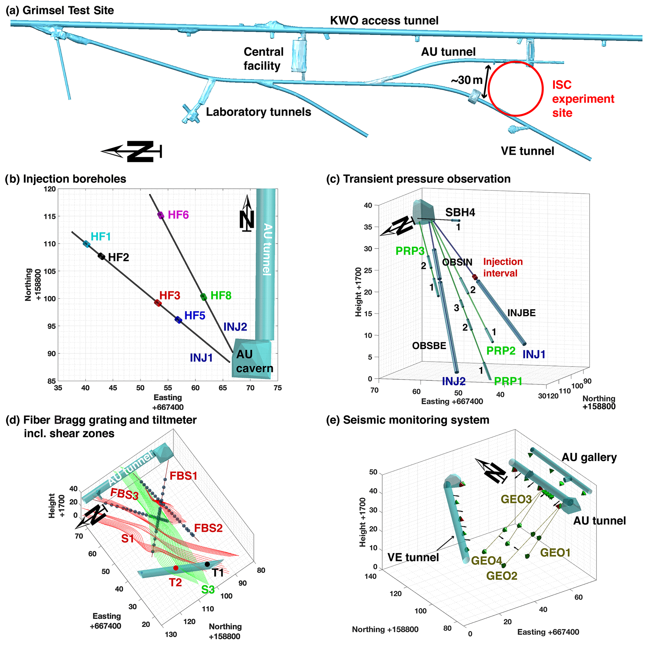
Figure 1(a) The ISC experiment site is indicated in the south of the Grimsel Test Site laboratory facility. (b) The AU cavern, the AU tunnel, and the injection interval locations in the two injection boreholes are shown and numbered. (c) Transient pressure observation intervals in six different boreholes. (d) Rock mass monitoring systems like fiber Bragg grating (FBG) sensors are indicated by blue circles in the three FBS boreholes, and tiltmeters are indicated by T1 and T2. The two different shear zones S1 and S3 are indicated by red and green. (e) The seismic monitoring system consists of accelerometers (red cones) and acoustic emission sensors (green cones) with eight sensors placed in four geophysical monitoring boreholes. Coordinates on panels (b) to (e) are referenced to the Swiss metric coordinate system (CH1903).
2.2 Geological characterization
The ISC test volume is situated slightly south of the boundary between Central Aare Granite (towards north) and Grimsel Granodiorite (towards south). Alpine deformation and metamorphism overprinted both lithologies, resulting in a pervasive foliation oriented 157/75∘ (dip direction/dip given in xxx/xx∘) (Keusen et al., 1989). See Wenning et al. (2018) for a detailed description of the rock mass in the GTS vicinity and its deformation history, including a comprehensive reference list. Tunnel mapping in the AU, VE, and AU-UP gallery was conducted to identify the main structures. The 15 boreholes drilled as part of the ISC project were logged with an optical televiewer to provide quantitative and qualitative information on the lithology, foliation, and fractures. Based on these data the main preexisting shear zones have been interpolated within a 3-D geological model (Fig. 2b).
The moderately fractured rock mass is crosscut by two sets of shear zones that differ in terms of deformation history and orientation. The first set (referred to as S1.0, S1.1, S1.2, and S1.3) included four ductile shear zones that are characterized by a strong increase in the degree of foliation and mylonitization. All four shear zones have an ENE–WSW strike and dip towards SE. These shear zones experienced retrograde brittle deformation and thus contain few discrete brittle fractures. The second set (referred to as S3.1 and S3.2) contains two brittle–ductile shear zones. The S3 brittle–ductile shear zones consist of a densely fractured zone (>10 fractures per meter) between two biotite-rich metabasic dykes.
Three lower-hemisphere equal-area pole stereonets with Kamb contour plots present each fracture as a pole point within the host rock and the associated shear zone S1 and brittle–ductile shear zone S3 (Fig. 2a). The pole points for the host rock and the S1 shear zone indicate a fracture system with a consistent horizontal NNW orientation with a tendency toward higher variation in the host rock. The fractures of the ductile–brittle S3 shear zone indicate two different fracture systems (Fig. 2a).
Figure 2d shows the fracture frequency, corrected into volumetric fracture density (p32) to account for sampling biases (see Brixel et al., 2019, for the correction), for the two injection boreholes, which indicates a moderately fractured rock mass. The fracture frequency in the INJ boreholes is zero to three fractures per meter, with higher frequency towards the shear zones. All obtained geological data and the interpolated 3-D model were published by Krietsch et al. (2018).
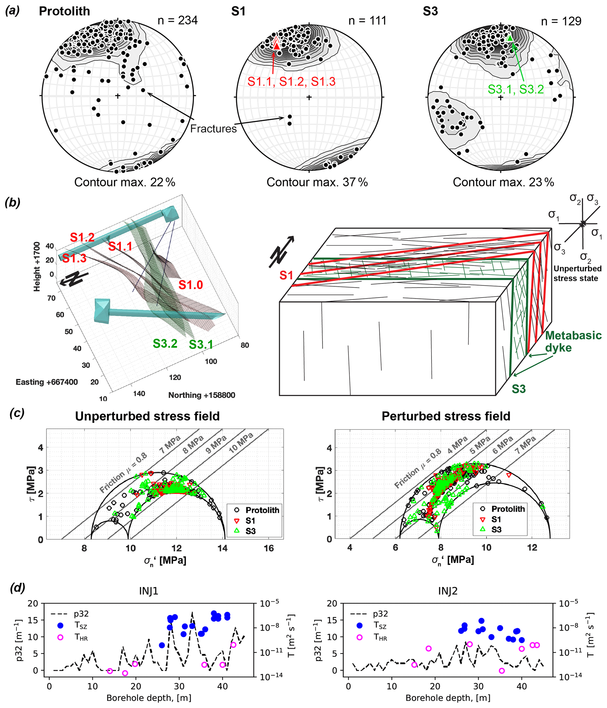
Figure 2(a) Kamb contour plots of fracture orientation projected on a lower-hemisphere equal-area pole stereonet for the intact rock (host rock), the ductile shear zone S1, and the brittle–ductile shear zone S3. (b) Geological model and block model for the ductile shear zone S1 and the brittle–ductile shear zone S3. The models indicate the different fracture systems associated with the two shear zones. (c) Mohr–Coulomb diagram representing the unperturbed and perturbed stress field estimate by Krietsch et al. (2019b) (including hydrostatic pressure of 0.3 MPa). The failure limits assuming a friction coefficient of 0.8. The identified and allocated fractures from borehole logging in all 15 boreholes are presented to indicate possible failure at a specific pore pressure (grey solid lines). (d) The black dashed line indicates the volumetric fracture intensity calculated over 1 m intervals for both injection boreholes INJ1 and INJ2. The magenta open and blue filled points indicate the position of well tests with the resulting transmissivities from fractured (TSZ) and intact rock (THR).
2.2.1 Stress characterization
Details of the stress characterization campaign are given by Krietsch et al. (2019b). Impression packers and microseismic monitoring were used to map hydraulic fracture orientation, which revealed consistent E–W, subvertical fracture extension. The averaged stress field in relatively unperturbed rock (i.e., with little fracture density) about 8 m from the S3 shear zones (Fig. 1c) and the perturbed stress field are summarized in Table 1. Hence, the minimum principal stress magnitude, measured in the subhorizontal borehole SBH4 approaching the S3 shear zone at the borehole bottom, is reduced towards the S3 shear zone (Krietsch et al., 2019b). This study will show that the perturbed stress state can be extended from the S3 brittle–ductile shear zone towards the S1 shear zone. The two main changes compared to the perturbed stress field are (1) a primary 30∘ clockwise rotation accompanied by a decrease in the major principal stress dip and (2) a permutation of the intermediate and minimum stress axis.

Figure 2c presents a Mohr–Coulomb circle for the unperturbed stress state considering the observed hydrostatic formation pressure of 0.3 MPa. Four different failure limits are presented between 7 and 10 MPa of overpressure, assuming a friction coefficient of 0.8 and no cohesion. Fractures and faults mapped from all 15 boreholes are sorted into three categories based on their relation to the main S1 or S3 structures and presented to estimate their criticality due to the fluid pressure increase. Structures favorably oriented for failure will fail with overpressures ranging from 8 to 10 MPa. All the HF experiments are located around the S3 shear zone, which influences the stress field as observed during the stress characterization campaign. To investigate this effect a Mohr–Coulomb circle for the perturbed stress state is presented and the failure limits are indicated for 4 to 7 MPa of overpressure. The perturbed stress field would allow for the shearing of structures above 4.5 MPa of overpressure, which is significantly below the observations from the unperturbed stress state. It is not clear which of the two observed stress states describes the injection into the rock volume approaching the S3 and S1 shear zones best. The experiments executed in borehole SBH4 approaching the S3.1 shear zone indicate a change towards the perturbed stress state.
2.2.2 Hydraulic characterization
Multiple field tests were performed to characterize hydraulic conditions at and near the injection borehole pair, including dilution tests and single-hole and cross-hole hydraulic tests. The transport properties of the conductive fractures were characterized using salt and DNA tracer tests (Jalali et al., 2018b). An overview of the hydrogeological baseline conditions for the ISC project is presented by Brixel et al. (2019). Hydrogeological conditions prior to the hydraulic fracturing experiment may be summarized as follows.
-
The transmissivity of the intact injection intervals (defined here as intact lithology by the absence of visually detected brittle deformation on cores and borehole image logs) was estimated through hydraulic pressure pulse tests and ranges from 10−13 to 10−11 m2 s−1 (pink circles in Fig. 2d). In injection intervals intersected by shear zones, constant rate injections (CRIs) or pulse injections (PIs) indicate higher transmissivity values of the order of 10−6 to 10−13 m2 s−1 (blue dots in Fig. 2d). The geometric average transmissivity of the host rock is estimated to be 10−11 m2 s−1.
-
The estimated transmissivities are in good correlation with the fracture intensity in the injection borehole INJ1 (Fig. 2d, left), although the spatial resolution of our hydraulic measurements do not permit the capture of all fracture intensity peaks. These measurements are also dependent on the natural heterogeneities, particularly related to the S1 shear zones. More details on these complex relations can be found in Brixel et al. (2019).
-
Within the brittle fractured zone between the two S3 shear zones an average discharge into the GTS tunnel of ∼60 mL min−1 was measured prior to the injection experiments.
-
Based on the characterization tests conducted, the fractured zone between and along the two S3 metabasic dykes provides the most conductive, natural flow pathways between the two injection boreholes. This observation agrees well with the existence of two different fracture systems in the S3 shear zone: (i) one set following the main NE–SW alpine foliation orientation and (ii) one set abutting the two S3 dykes at high angles, which we identified as the alpine tension gashes commonly mapped between dyke swarms throughout the Grimsel Test Site (Fig. 2a, right). This rock volume contains open fractures with high transmissivity (i.e., extension fractures), whereby the transport of solutes, salt, and DNA tracers between the two injection boreholes shows a preferential pathway towards the gallery rather than towards the INJ1 borehole for the case of injection into INJ2 (Jalali et al., 2018b).
Hydraulic fracturing experiments conducted within this study were accompanied by an extensive monitoring program including measurements of rock deformation, fracture fluid pressure, and microseismicity. In the following sections, we introduce the hydraulic fracturing equipment and the monitoring systems.
3.1 Hydraulic fracturing equipment
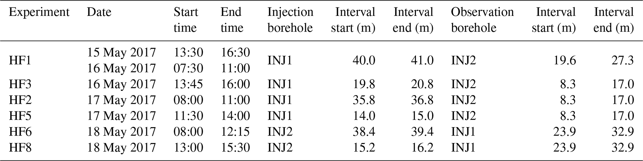
The HF interval was isolated using a hydraulic double-packer system with a 1 m long pressurization interval. Two different triplex pumps (brand SPECK Pumpen) were used to deliver (1) a pressure up to 30 MPa at a flow rate up to 35 L min−1 and (2) a flow rate up to 100 L min−1 at a maximal pressure of 10 MPa. The first pump was used to break down the formation and for the first propagation cycle. Then, the pump was switched to reach flow rates up to 100 L min−1. A second double-packer system was installed to monitor the fluid pressure response in the monitoring interval in the second injection borehole that was not used for active stimulation. A data acquisition system recorded the pressure in the open intervals of the INJ boreholes, the flow rate in the injection interval, and the packer pressure in the injection and monitoring intervals with a sampling rate of 20 Hz. Fluid pressure was also monitored in the intervals beneath the injection and monitoring intervals with a sampling rate of 1 Hz. The injected fluid and the backflow were measured with different flowmeters depending on expected flow rates with a sampling rate of 20 Hz. Figure 1b presents the position of the six injection intervals along the two injection boreholes INJ1 and INJ2. As a visual aid, we used consistent color throughout the paper to display data from a specific HF experiment. The execution times and the intervals for all experiments are summarized in Table 2.
Table 2Overview of the executed experiment and borehole location, depth of testing interval, and observation depth interval.
3.2 Monitoring systems
The pressure monitoring system was designed to observe transient pressure response at specific locations to track pressure propagation throughout the rock mass, either through natural fractures or newly created ones. Customized grout packer systems were installed in the PRP monitoring boreholes. The open intervals were packed and separated with hydromechanical packers supplemented with resin. The uppermost interval was filled with grout to ensure low compressibility of the system. Open hole sections are shown as blue cylinders in Fig. 1d. The sections PRP1-1, PRP2-1, and PRP3-1 are positioned within shear zone S1, and all the other intervals are positioned within shear zone S3. The pressure sensors (PAA33-X Keller) were connected to the Solexpert data acquisition system running the Solexpert GM-HF software with a maximum sampling rate of 20 Hz. The possible pressure range of the pressure sensors was up to 10 MPa with a resolution <1 kPa. The raw pressure data from HF stimulations are presented in the paper without any filtering.
The rock mass deformation monitoring system consists of 60 fiber Bragg grating (FBG) sensors (type os3600 by Micron Optics, Inc.) in the three FBS boreholes. The FBG sensors have a base length of 1 m; 20 FBG sensors were installed along each FBS borehole to characterize the strain field in both intact and fractured rock. The sensors (including strain and temperature) are pre-strained to about 2000 microstrains such that shortening can also be recorded. The sensors were connected to an interrogator of type si255 (Hyperion Platform by Micron Optics, Inc.) that can record with a sampling rate of 1 kHz, an accuracy of 0.85 microstrains, and wavelength repeatability of 0.1 microstrains. The strain data presented here are not temperature-corrected as they are not required for our isothermal injections. Extensional strain is negative.
Two tiltmeters (type A711-2 by Jewell Instruments) were installed in the VE tunnel to characterize the deformation with respect to the stimulation volume. The location of each tiltmeter is presented in Fig. 1c. The tiltmeters measure the deviation from horizontal tilt in the axial (x) and normal (y) direction to the tunnel with a resolution of 0.05 µradians after filtering with a 100 Hz low-pass filter. The two horizontal tilt axes and the temperature were digitized and recorded by the data acquisition system with a sampling rate of 100 Hz. The initial value was subtracted to display the change in tilt during the HF experiment. Then, a positive tilt in the x axis implies a dip of the tunnel wall towards NNE. A positive dip in the y axis indicates a dip of the tunnel floor towards WNW.
The seismic monitoring network consists of a total of 26 uncalibrated piezoelectric acoustic emission (AE) sensors (type GMuG Ma-Bls-7-70m) and five calibrated accelerometers (type Wilcoxon 736 T) (Fig. 1e). The AE sensors have a bandwidth of 1 to 100 kHz, and their highest sensitivity at 70 kHz. Eight of the AE receivers were deployed in four geophysical boreholes (GEO) in close proximity (3–25 m) to the injection intervals. The accelerometers have a bandwidth of 5 to 25 000 Hz with a sensitivity of 100 mV g−1. The seismic data were recorded continuously throughout the experiments at a sampling rate of 200 kHz using a 32-channel acquisition system. AE and accelerometer receiver signals were high-pass hardware-filtered at 1 kHz and 50 Hz, respectively.
Based on the picked P-wave onsets, the seismic event locations were calculated using a homogeneous but transversely isotropic P-wave velocity model. For more details on the seismic monitoring and event localization, see Doetsch et al. (2018b), Gischig et al. (2018), and Villiger et al. (2019). The experimental summary cards in the Supplement (Figs. S8 to S13) present the located seismic events and their radial distance to the injection interval. Time synchronization of all data acquisition units used for the HF injection tests was ensured using a network time protocol server.
4.1 Injection protocol
The HF injection experiment was executed between 15 and 18 May 2017. The injection protocol showing the injected flow rate (blue line) and the injection pressure (red line) for each HF experiment is presented in Fig. 3. The grey shaded regions in the plots correspond to the phases of fluid injection. Prior to the first injection phase of each experiment, a pulse injection was executed to test interval integrity and packer sealing. The actual hydraulic fracturing experiment started with a rate-controlled fluid injection at approximately 5 L min−1 for 10 s to initiate a hydraulic fracture. This formation breakdown cycle (frac cycle) is indicated by the letter F in the injection protocols and consists of the fluid injection, the pressure observation during shut-in time, and fluid recovery during bleed-off time.

Figure 3The injection protocol of the different HF experiments is presented showing the flow rate (blue line) and the injection pressure (red line). The grey shaded sections correspond to fluid injection into the interval. Experiment HF1 was divided into two protocols due to water supply problems during the first day. The protocols (a)–(g) follow the temporal execution in the field. For the experiments in (a)–(d) the injection fluid was water during the fracture propagation cycles (RF1–RF2), and for the experiments in (e)–(g) the injection fluid was a xanthan–salt–water mixture.
The two following refrac cycles RF1 and RF2 had the aim of propagating the hydraulic fracture. During these cycles, we used either water with a viscosity of 1 cP (10−3 Pa s) (Fig. 3a–d; experiments HF1, HF2, and HF3) or a shear-thinning fluid (xanthan–salt–water mixture or XSW) with a viscosity of ∼35 cPs (Fig. 3e–g; HF5, HF6, and HF8). The refrac cycle RF1 starts with a flow rate of 5 L min−1 which was progressively increased to 10 and 20 L min−1. Each step lasted for approximately 2 min or less. For the experiment with water, we performed a cyclic injection during the 20 L min−1 step. The cyclic injection consisted of a sinusoidal variation of flow rate with a period of 2.5 to 20 s and an amplitude of ±15 L min−1. Following the 20 L min−1 injection step we increased to 35 L min−1 for 3 min. Then, the system was shut in to change to the bigger pump, and injection was resumed without bleed-off with a second propagation cycle called RF2.
The refrac cycle RF2 begins with a rapid increase in the flow rate to 35 and then increased to 50 L min−1. Both flow steps were maintained for 2 min. Afterward, each step was held for 1 min starting from 60 L min−1 and going up to 70, 80, 90, and 100 L min−1. The system was then shut in for several minutes to half an hour to observe the hydromechanical response in the system. Finally, the system was opened to allow bleed-off. The fluid recovery rate was monitored. For the HF experiments with XSW fluid (HF5, HF6, and HF8), we added a third refrac cycle RF3 with clean water with the aim of flushing out the XSW fluid. The water was injected at 35 L min−1. This cycle was also an opportunity to test different cyclic injection schemes. The fluid injection was again followed by shut-in and bleed-off phases. For all experiments, the last cycle was a pressure-controlled step test (SR) to evaluate the post-stimulation injectivity of the created hydraulic fracture and to estimate the stress acting normal to the hydraulic fracture (jacking pressure) based on Doe and Korbin (1987). For the executed injection protocols, the following remarks are noted.
-
Logistic problems affected the execution of the HF1 experiment. The issue was an insufficient water supply. This led to several repetitions of the refrac cycle RF1. The second refrac cycle (RF2) was then executed a day later with a newly installed water supply pump delivering the necessary flow rates. Furthermore, the seismic monitoring system recorded an increased quantity of electronic interference due to faulty shielding of the power line between the frequency control unit and pump motor. Therefore, a seismic evaluation was not possible.
-
At a flow rate of 5 L min−1 during the first refrac cycle of experiment HF5, a shortcut occurred to one of the open seismic monitoring boreholes (GEO1; Fig. 1e). For this reason, we had to interrupt RF1 and resume multiple times. This is why RF1 is subdivided in panels (a), (b), and (c) in Fig. 3. Thereafter, the pump was changed to allow for flow rates above 35 L min−1, but the flow rate was limited to a maximum of 80 L min−1 and a short duration due to the shortcut to the GEO1 borehole. The flushing cycle RF3 was executed with a flow rate of 50 L min−1.
-
The low magnitude of breakdown pressure during the frac cycle of HF6 is an indication for a preexisting sealed fracture in the open interval. The stimulation interval was mistakenly placed 3 m further down in the borehole at a preexisting fracture.
-
During all refrac cycles, we never exceeded an injection pressure of 10 MPa.
-
Experiments HF3, HF5, and HF8 show a similar fast pressure decay during the shut-in time for the refrac cycles. The same experiments show very small fluid recovery (fluid recovery is shown as negative flow rate in Fig. 3) after the refrac cycle RF2 compared to the experiments HF1, HF2, and HF6.
4.2 Diagnostic injection parameters
Table 3 summarizes key observations from the injection protocol (labeling after Fig. 3). The measurement of breakdown pressure, fracture reopening, and instantaneous shut-in pressure (ISIP) followed the International Society for Rock Mechanics (ISRM) standard presented by Haimson and Cornet (2003). The breakdown pressure represents the peak pressure during injection cycle F. The instantaneous shut-in pressure was obtained during each cycle using the tangent method, i.e., the departure from a linear pressure decrease vs. time occurring right after shut-in (Amadei and Stephansson, 1997). The apparent reopening pressure (Pr) was picked when the pressure change–time step relationship starts being nonlinear (Bredehoeft et al., 1976). The jacking pressure was measured during the pressure-controlled step test SR (more in the Supplement, Sect. S1). The cumulative injected water corresponds to the injected volume, Vi, indicated for each cycle and the entire experiment. The backflow was measured at the injection interval during venting. Thus, the fluid recovery Vr is only the recovery from the injection interval; however, fluid also escaped from two of the monitoring boreholes (GEO) during the HF5 and HF8 experiments and from the fractured zones during all experiments. These outflows were also monitored to validate the overall fluid balance over each experiment. Cycle RF1 for HF1a and HF5 correspond to multiple refrac cycles. Thus, the reopening pressure and the ISIP were averaged, and the fluid injection and recovery are presented as a cumulative number.
Table 3Overview of fracture breakdown pressure (Pc), fracture reopening pressure (Pr), additional hydraulic test parameters (injected fluid: water (W) or xanthan–salt–water mixture (XSW); Vi, injected volume; Vr, recovered volume), and located AE event numbers.

NA – not available.
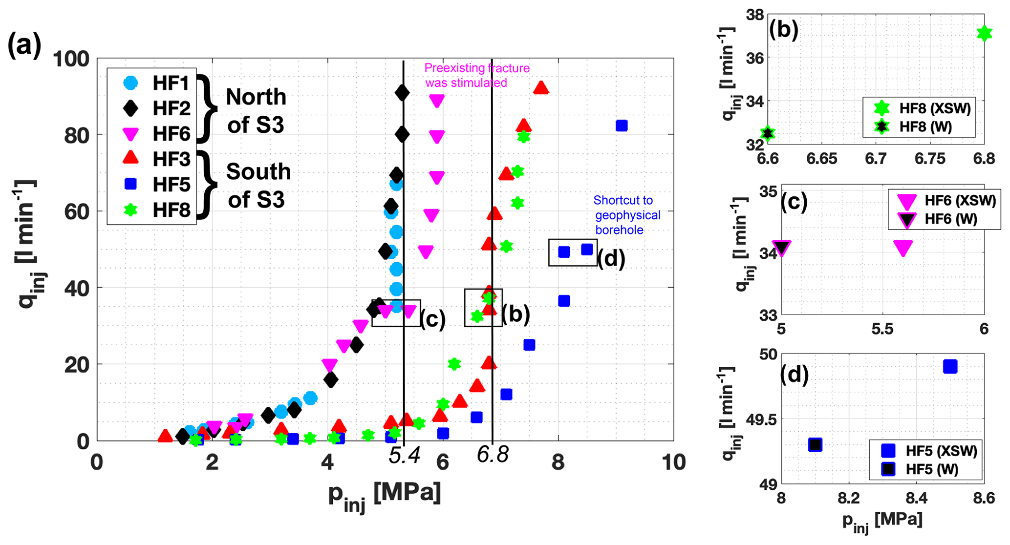
Figure 4(a) The injection flow rate qinj vs. interval pressure pinj at pseudo-steady state from the second refrac cycle RF2 and pressure-controlled step test SR (similar to Fig. S1 in the Supplement) for all HF experiments. The black solid lines indicate a limiting pressure behavior for HF1–HF2 and HF3. Panels (b–d) highlight the pressure drop when changing from XSW to water with a similar flow rate.
Figure 4a presents the flow rate (qinj) vs. the interval pressure (pinj) at pseudo-steady state for the second refrac cycle RF2 and the pressure-controlled step test for each HF experiment. For any injection step, the injection conditions (either controlled flow rate or constant pressure) were maintained until a stable state was reached, i.e., quasi-constant pressure for rate-controlled injections or quasi-constant flow rate for pressure-controlled injections. While we acknowledge that true steady-state conditions are never reached in practice, we took the latest data point prior to starting the next step of our injection. A major observation is that there is a clear difference between HF experiments executed south of the S3 shear zone (HF3, HF5, and HF8) and north of the S3 shear zone (HF1, HF2, and HF6). HF1 and HF2 were located in the S1 shear zone and reached a pressure-limiting behavior at an injection pressure of 5.4 MPa for flow rates larger than 35 L min−1 (Fig. 4a). During these two experiments, only two propagation cycles (RF1 and RF2) were executed. Considering experiment HF6, the pressure-limiting behavior occurred at a higher pressure of 6 MPa.
HF3, HF5, and HF8 were located south of the S3 shear zone. In general, all experiments executed on this side of the S3 shear zone had higher injection pressure. HF3 and HF8 similarly showed a slight increase after reaching a flow rate of 10 L min−1. The injection pressure reached a limiting pressure of 7.8 MPa. The injection fluid for HF3 was water and for HF8 XSW followed by an additional flushing cycle using water. Experiment HF5 showed the highest increase in injection pressure for increasing flow rate with a maximum injection pressure above 9 MPa. The pressure dropped to around 0.5 MPa at the same flow rate (35 L min−1 or 50 L min−1) using XSW during the refrac cycle RF2 and the flushing cycle (RF3) using water for experiment HF6 and HF5. The effect is smaller for HF8 with a pressure drop of only 0.2 MPa. Therefore, we can infer that the viscosity effect (i.e., the change of XSW to water) results in a decrease in injection pressure, but further investigation is necessary to reliably quantify the effect. For the sake of clarity, the flow rate and pressures from the flushing cycle associated with the pressure drop are presented in Fig. 4b–d.
The limiting pressure is smaller compared to the hydraulic tensile strength calculated from the difference between breakdown and reopening pressure (Bredehoeft et al., 1976), ranging between 8.3 and 9.6 MPa. The tensile strength measured by Dutler et al. (2018) ranges between 5.6 and 14.7 MPa for the transversely isotropic host rock. Therefore, the hydraulic tensile strength depends on the orientation of the isotropic plane. The limiting pressure ranges between 5.4 MPa (HF1 and HF2) and 6.8 MPa (HF3) and is interpreted as reflecting conditions when the fracture surfaces have fully lifted off near the wellbore. However, it is questionable if the hydraulic fractures still extend (creating new surfaces) at this pressure.
The difference from HF6 to the two other injection experiments (HF1 and HF2) may be due to two reasons: (1) the HF6 interval contains a preexisting fracture that may not be perpendicular to the minimum principal stress. (2) The injection fluid in HF6 is XSW. Thus, the pressure reaches higher values as pressure dissipation is affected by the high fluid viscosity. During the flushing cycle of this fracture (RF3), a pressure decrease was observed, reflecting a viscosity effect.

Figure 5The black solid line in all plots indicates the S3 shear zone, which divides the experiments in north (N) and south (S) with a pseudo-distance ordering of the HF experiments on the y axis from the top of the borehole (HF5) to the end (HF1). (a) ISIP from the frac–refrac cycle and the best estimate of jacking pressure (JP). (b) The injected and backflow volume are presented for the three main refrac cycles for each experiment. No recovery phase took place after RF1. (c) The final matrix injectivity from the pressure-controlled step test. (d) The initial transmissivity was measured from pulse injection prior to the HF experiment, and the final transmissivity was measured via constant head injection several weeks after the experiment.
Figure 5 presents four subplots summarizing (a) the ISIP and JP, (b) the injected volume and backflow, (c) the final injectivities before jacking derived from the analyses of the SR cycles, and (d) the initial and final transmissivity derived from hydraulic experiments performed prior to and after the HF experiment. Figure 5a compares the ISIP obtained during the frac–refrac cycles with the jacking pressure. The ISIP varies between 5.5 and 7.9 MPa for the frac cycle and decreases with ongoing refracturing. For all experiments, the ISIP stabilizes around 5 MPa and shows slightly higher values between 4.5 and 6.5 MPa for experiments executed south of S3 (above the black solid line) and values between 4.0 to 6.0 MPa for experiments executed north of the S3 shear zone. South of the S3 shear zone, the jacking pressure reaches values between 5.1 and 6.0 MPa, which is comparable with the ISIP from the refrac cycles. In contrast, the jacking pressure north of S3 ranges between 3.0 and 3.7 MPa for the experiments executed. This reflects 1 to 2 MPa smaller values than using the ISIP from the refrac cycle (Fig. 5a).
The injection volume and the recovery volume from the injection intervals for the main fracture propagation cycles RF1–RF2 and the flushing cycle RF3 are presented in Fig. 5b. The injection volume for each cycle is similar for all experiments except HF1. For HF1 the injection protocol was stopped after refrac RF1 and continued the following day. After the first propagation cycle, no fluid recovery took place. Both the second fracture propagation cycle RF2 and the flushing cycle RF3 show minor or no backflow from the injection interval for the experiments executed south of S3 (>2 %). In contrast, for the experiments executed north of S3, the recovered fluid from the injection point reaches values between 15.0 % and 23.5%. Experiment HF6 reached the largest volume recovery of all experiments: during the flushing cycle RF3 a recovery of 74.3 % was observed. The final injectivity before jacking is presented in Fig. 5c and ranges between 2.77 and 3.69 north of S3 and between 0.21 and 0.88 south of S3. Approaching the S3 shear zone from the south, injectivity values increase. The experiments located further down in the borehole show the highest injectivity values, which correlates directly with an increase in fracture density in the shear zone S1.
4.3 Transmissivity values from pre- and post-HF hydraulic tests
The change in transmissivity at the injection interval was investigated by packer testing before and after the HF experiment in borehole INJ1 and INJ2. Prior to the HF experiment, pulse injection (PI) tests were performed, and after the HF experiment constant head injection (CHI) tests were performed. To estimate the equivalent hydraulic parameters (transmissivity and storativity), the PI tests were inverted with the n-dimensional Statistical Inverse Graphical Hydraulic Test Simulator, nSIGHTS (Roberts, 2006), and the CHI tests were analyzed using the Jacob and Lohman (1952) solution. For both methods the radius of influence is different, and therefore the numbers are only an indication of permeability enhancement and not for direct comparison. The initial magnitude of local transmissivity estimates ranges m2 s−1. Final transmissivities after the HF experiment from CHI tests reach values of m2 s−1. HF6 is an exception as it took place at a preexisting fracture, for which transmissivity was not measured before the HF experiment. The final transmissivity for HF6 is highest in magnitude for all HF experiments with m2 s−1. There is a trend of 1 magnitude higher transmissivities after HF for experiments on the northern side of the S3 shear zone (more in the Supplement, Sect. S2).
4.4 Borehole fracture trace
Prior to the HF experiments, analyses of drill cores and optical and acoustic televiewers have been carried out to select appropriate test intervals. Suitable test intervals for hydraulic fracturing were selected if no preexisting fractures were visible. Figure 6 presents the amplitude log from the acoustic borehole televiewer for the six HF intervals for pretesting and posttesting. The travel time log is not presented as no changes were recognized. The blue highlighted section in the center indicates the injection interval, which does not show any fractures prior to testing, except for HF6. The areas below and above the blue section show the location of the straddle packer of 1 m length. The preexisting fractures are indicated in green and located at the straddle-packer emplacement. The new fracture trace is indicated by a red arrow. The dip and dip direction were determined by fitting a sinusoidal trace using the WellCAD software by Advanced Logic Technology. Based on the probe orientation measurements, the true orientations of the induced fractures were computed. Travel time data accuracy that allow, at best, for the resolution of radius changes of 0.15 mm do not allow for the quantification of wellbore deformation associated with the presence of the newly created fracture trace, but changes in signal amplitude are sufficient to identify the newly created features during the HF experiments. The borehole traces are either axial to the borehole or have a steep angle to the borehole axis not exceeding 20∘. An exception is found in the post-log of HF1, which indicates new en échelon structures for one side of the fracture trace and mostly likely a packer-induced fracture trace towards the bottom of the HF interval. These structures are a result of the deviated borehole with respect to the perturbed stress tensor (Table 1). We recognized that for all HF experiments many of the new fractures extend below the straddle packer and stop at a preexisting fracture.
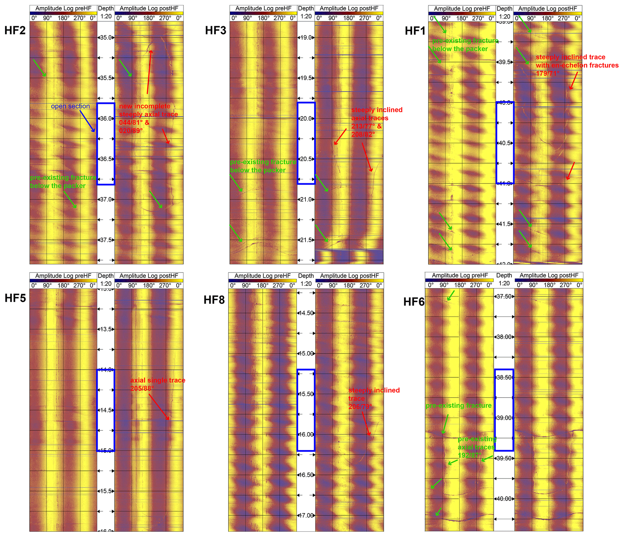
Figure 6Pretesting and posttesting acoustic borehole televiewer (ATV) logs of the borehole INJ1 and INJ2. The blue highlighted sections in the center indicate the open intervals that do not show any fractures prior to testing except for HF6, which was stimulated at the wrong position. The preexisting fractures are indicated with green arrows. The areas below and above the blue section show the location of the straddle packers. Five of six experiments show new features in the posttesting images, which indicates an induced fracture.
4.5 Microseismicity
During the HF experiments, we detected in total 6986 microseismic events, 730 of which were located. P-wave arrivals were picked manually and located using an absolute location procedure including a joint hypocenter determination (JHD) and a homogeneous, transversely isotropic velocity model (P-wave velocity along the axis of symmetry 5195 m s−1, along the axis of isotropy 4865 m s−1). The relative uncertainty of location considering picking uncertainties lies in the range of ±1.5 m; absolute location uncertainties range from below 0.5 m in a depth interval from 15 to 30 m in INJ1 to 1.5 m towards the mouth and bottom of INJ1 and INJ2. Details on the analyzed induced seismicity are presented in Villiger et al. (2019). The number of located events for each frac–refrac cycle are indicated in the last row of Table 2. In Sect. S6 in the Supplement, each experiment is presented showing the injection protocol with flow rate and injection pressure, the located seismic events for each frac–refrac cycle in plane and profile view, and the cumulative injected volume, cumulative backflow, and the distance between injection point and located seismic events. Figure 7a presents the seismic clouds for five of the six hydraulic fracturing experiments (color-coded experiment-wise).

Figure 7Seismicity clouds in side view (a) and map view (b) including 3-D cylinders presenting the open injection intervals in the two injection boreholes. Each experiment has the same color for the seismicity points, 3-D cylinders, and labels.
The number of located seismic events for experiment HF5 and HF6 is very small. Most seismic activity is observed during experiment HF2 and HF8. Note that the location of the injection intervals with respect to the seismic sensors cannot explain the large difference in detected and located seismic events. During all experiments, the seismic events are located more often below the injection point than above. Also, seismicity propagates predominantly towards east.
A peculiar seismic pattern was observed during HF2 (see Fig. S9 in the Supplement): seismicity radiates away from the injection point up to a distance of about 5 m during the first part of refrac cycle (RF1) and then propagates to about 10 m away from injection. However, during the second refrac cycle (RF2), seismicity resumes 10 m away from the injection point and develops toward the injection point. This behavior is atypical since migration away from the injection point is typically expected and observed.
Seismicity occurred during all frac–refrac cycles for HF8. Most of the seismic events were observed during the first refrac cycle. The events were located around the borehole with a maximal radial distance of only 10 m. Only three events were located further away during the same cycle. Refrac cycle RF2 and RF3 show less seismic activity compared to RF1, which occurs further away from the injection point.
During the two refrac cycles of HF3, 75 located seismic events occurred. These located seismic events show a dispersed pattern. Most of the seismic events appear below 10 m of radial distance from the injection point. Generally, minor seismicity is related to the refrac cycle RF3 and no seismicity is associated with the pressure-controlled step cycle SR for all experiments except HF6.
4.6 Fracture geometry
The seismic event locations are shown in a stereographic projection centered on the injection point in Fig. 8. Here, each seismic event is represented by the intersection of a unit sphere centered on the middle of the injection interval and a line connecting this middle point and the location of the seismic event. With this method, each seismic event is presented as a point on a lower stereographic projection for experiment HF2 and HF8, respectively (Fig. 8). The color of the circle indicates the frac–refrac cycles. In this representation, the location uncertainty of the seismic events strongly impacts the event orientations close to the injection point. A color saturation scheme is used to give less importance to these events: a more intense color is used for events located farther away from the injection point and linearly decreasing the color saturation towards the injection points. Events located within a radial distance of 1 m (typical location error for our seismic events) from the injection point are not represented.
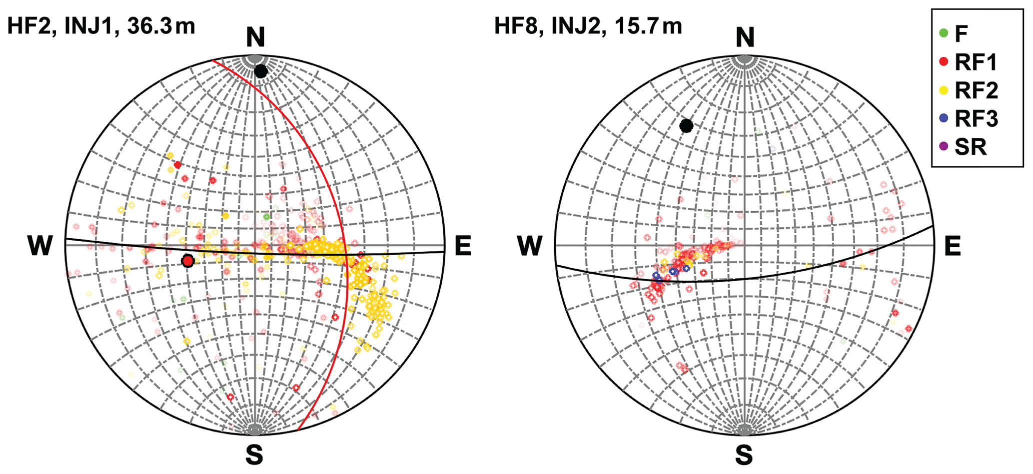
Figure 8The center of the lower stereographic projection corresponds to the injection point and each circle to a seismic event. Circles with a white face color and a different edge color are projections on the lower stereographic net, and fully colored circles are projections on the upper stereographic net. The girdle pattern indicates the fitted planes including the pole point for different seismic clusters (colored pole point). Considering all seismic events, the girdle pattern and the pole point are black.
In the idealized case of symmetric radial extension of the seismic cloud on a plane from the injection point, the expected pattern on the stereoplot would be a girdle pattern, i.e., all the points will line up on a circle in the stereoplot. In Fig. 8 we present the best-fit plane (for the method and results see Sect. S5 in the Supplement) through the seismic cloud via a girdle pattern for all seismic events (black pole point for HF8) and for two clusters (i.e., RF1 and RF2 for HF2, red and yellow pole point). The two HF experiments presented in Fig. 8 do not follow this idealized pattern. In our case, the points tend to cluster, which represents a linear structure.
For HF2 during RF1 (red), the points tend to distribute on an E–W subvertical plane and cluster on a linear structure dipping about 70∘ to the east. During RF2, the seismicity cloud migrates (yellow) towards a well-defined linear structure with a dip of 25∘ to the ESE. The means from the first and second refrac cycle are very consistent, dipping 40 to 50∘ to the east. The seismicity cloud of HF8 is clustered on a linear structure dipping 60 to 70∘ to the west. Most of the seismic events take place during refrac cycle RF1 and RF2, with more intense color saturation as they are located further away from the injection point. The means of refrac cycles RF1 to RF3 are very consistent for experiment HF8.
4.7 Hydromechanical observations
Two experiments, one executed north of S3 (HF2) and the other one south (HF3), are presented and compared here in terms of deformation and hydraulic pressure distribution in the rock mass. Similar information on the other experiments can be found in Sect. S3 in the Supplement. For the two experiments presented here, the injection fluid was water and the injection intervals were devoid of fractures prior to stimulation.
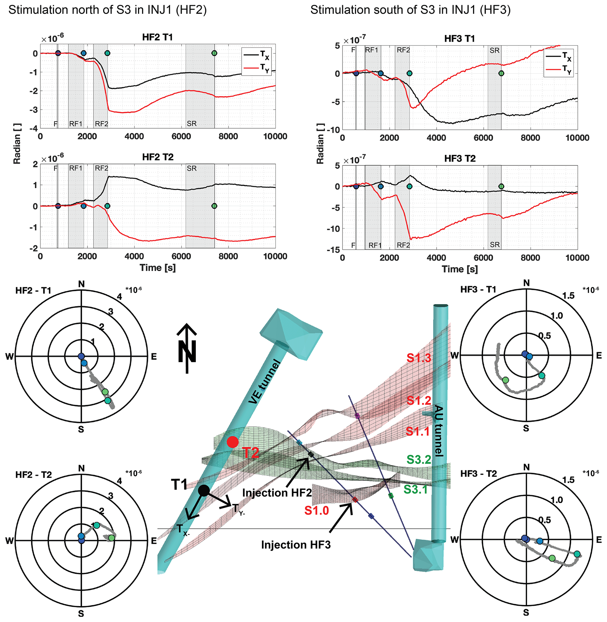
Figure 9The time series of tiltmeters T1 and T2 are presented for experiments HF2 and HF3. The fluid injection is indicated by the grey boxes. The colored points at the end of fluid injection in the time series are presented in a polar plot. The magnitude of the circles in the polar plot are given in radians. The sketch shows the injection points, the orientation of the shear zones, and the tilt device location with negative tilt magnitude parallel Tx− and perpendicular to the tunnel Ty−.
The tiltmeter data (Figs. 9 and S3) measure the deviation of the VE tunnel floor from horizontal. The fluid injection is presented by grey shading in the time series of the tilt data. In general, the largest tilt is related to higher injection rates and increasing fluid volume. The magnitude of the tilt axis globally ranges between −4 and 3 microradians. The magnitude of the tilt signals decreases with respect to the injection location and shear zone as follows. Injections executed south of S3 show in general smaller magnitudes in tilt than the one executed next to S1, as they are farther away from the tiltmeter locations. Also, the response of the tilt signals reacts either instantaneously or delayed depending on the location of injection (distance-controlled response). The experiments next to the shear zone S1 in borehole INJ1 (HF1 and HF2) show an instantaneous response in the tiltmeter T1 and a delayed response in the y component of tiltmeter T2. We interpret the tunnel floor to be tilting away from the injection volume, which accumulates in the intersection zone of S1 and S3.
Tiltmeter T1 of the experiments south of S3 (HF3 and HF8) tilts away from the S1.2 shear zone, and T2 tilts along the strike of the S3 shear zone. Experiments executed south of S3 are expected to connect to the fracture system of the shear zone S3, which acts as a preferential flow path towards the AU tunnel.

Figure 10Selected time series of FBG sensors from borehole FBS1 and FBS2 for experiments HF2 (a–c) and HF3 (d–f) including the sensor location. The fluid injection time is indicated by the grey boxes. The depth of the sensors measured from the top is indicated in the specific legends from the time series. Positive strain indicates compression.
Figure 10 presents selected time series from the FBG strain sensors and the FBG strain data along the FBS boreholes at the end of refrac cycle RF1 and RF2 and the permanent change for the two aforementioned experiments HF2 and HF3. The strain data were set to zero at the beginning of the experiment, as we are interested in the relative changes during an experiment. A positive strain is associated with compression, and negative strain represents tension. The permanent strain was either measured 2 h after the experiment or at the starting time of the next experiment. The fluid injection is indicated by the grey boxes. The time series of HF2 of the FBG sensors at 31.8 and 33.0 m indicate a fast-tensional increase during RF1 linked to the arrival of the fluid front (i.e., the sensor at 33.0 m with one fracture along the sensor base length). The sensor at 31.8 m was placed in intact rock and indicated only compressional signals prior to the HF2 experiment. Therefore, it was hit by the hydraulic fracture during RF1. The highest tensional signals are observed in the S1 shear zone for experiments HF1, HF2, and HF6. Above 35 m the FBG sensors in FBS2, which are oriented parallel to the S3 shear zone and cross the S1 shear zone at 35 m, indicate compression above 35 m and tension below 35 m. This is directly related to fluid flow through fractures intersecting the base length of the FBG sensors related to the S1 shear zone.
The time series of HF3 in Fig. 10 show two FBG sensors at 22.35 m in FBS1 and at 20.0 m in FBS2 with very high transient peak strain. The time series of the FBG sensor at 20.0 m in FBS2 from HF3 indicates the largest transient peak strain during all HF experiments. Most of the observed peak strain is reversible, and 50 µϵ represents irreversible (permanent) strain. We assume that this tensional reversal strain is directly linked to the fluid pressure. The sensor at 23.35 m in FBS1 is located at the metabasic dyke. This sensor shows compression, whereas the sensors between the two metabasic dykes indicate tension (e.g., the sensors at 24.3 and 24.8 m). The high transient strain signals (i.e., FBS1 22.35 m and FBS2 20.0 m) indicate major flow paths and are only observed for experiments executed south of S3. In FBS2 only three FBGs observe tensional strain, while all the other sensors are compressed, with the highest compression towards the extensional section. Along the borehole FBS3, the sensors associated with S1 shears and intact rock show compression. Note that most of the tensional strain signals are observed on sensors associated with the brittle–ductile shear zone S3 (i.e., FBS1 23–30 m and FBS3 > 33 m). Large permanent strain changes are not observed (changes are in a range of 20 to −30 µϵ).
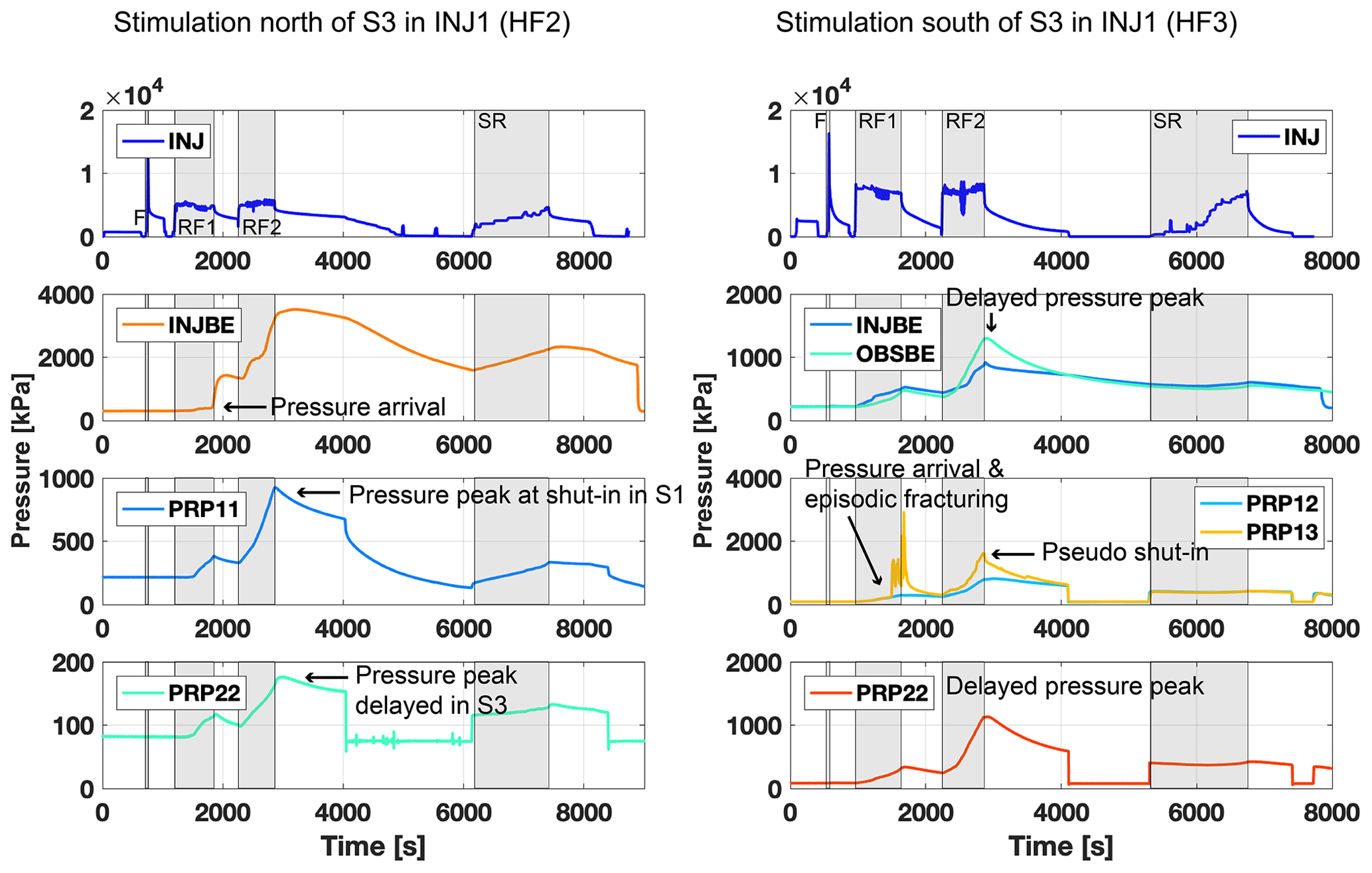
Figure 11Selected time series of pressure response are presented for experiments HF2 and HF3. The fluid injection is indicated by the grey boxes.
Selected time series from pressure observation intervals in the injection and observation boreholes are presented in Fig. 11 for the hydraulic fracturing experiments HF2 and HF3 (for the other experiments see the Supplement). The injection pressure (INJ) is presented on top including the grey boxes, which indicates fluid injection.
For the stimulations north of S3 (HF2) the time series from the interval below the injection (INJBE) shows a pressure arrival directly at the end of the first refrac cycle RF1. The peak of the pressure response in PRP1-1 is at the end of refrac cycle RF2. The interval PRP2-2 is located in the shear zone S3, and the injection location is next to the S1 zone. It is expected that the fractures related to the S1 zone are connected first, and therefore the interval PRP2-2 located in the S3 shear zone has a delayed pressure peak. The interval INJBE is located next to the injection interval (in shear zone S1.2 and S1.3), showing pressure arrival after cycle RF1. The nearly instantaneous pressure response indicates a new complex flow path connection to the injection interval below. In addition, the largest amplitude is observed compared to all other observation points, and the maximum peak after shut-in is delayed compared to interval PRP1-1. This indicates a longer fluid path reaching interval INJBE than PRP1-1.
The HF3 injection experiment triggered a strong signal during the first refrac cycle in the observation interval PRP1-3: it indicates an abrupt pressure arrival and an episodic pressure change during and after pump shut-off. At the end of cycle RF2, pseudo-shut-in is observed at the interval INJBE and PRP1-3: i.e., both pressure curves drop after pump shut-off. The pseudo-shut-in in the observation interval near the injection interval is a mechanical response starting from the injection interval due to instantaneous pressure loss. The observation intervals OBSBE and PRP2-2 respond with a delayed pressure peak, wherein the two intervals are located further away than the two intervals (INJBE and PRP1-3), showing pseudo-shut-in.
In the following section, we compare the hydraulic fracturing experiment with several small-volume (∼10 L) hydraulic fractures from the stress characterization phase (hereinafter called minifracs or MFs). The minifracs were accompanied by microseismic monitoring to investigate the initiation and propagation of the newly induced fractures. A detailed description of the stress characterization and the minifracs has been published by Gischig et al. (2018), Jalali et al. (2018b), and Krietsch et al. (2019a). In the separate experimental summary cards, each minifrac experiment from SBH3 and SBH4 boreholes is presented in a similar way as the HF experiments. A summary of the injection pressure and seismic characteristics of all MF experiments (SBH1, SBH3, and SBH4) can be found in Sects. S4 and S6 in the Supplement including an overview of the injection interval locations.
5.1 Injection pressure observations
Figure 12 summarizes the breakdown pressure and the ISIP from all MF and HF experiments. Breakdown pressure and ISIP decrease towards the S3 shear zone. The highest decrease is observed in borehole SBH4 approaching the S3 shear zone at the end of the borehole. The experiments executed in borehole SBH3 (MF1–MF3) show the highest breakdown pressure between 23.4 and 26.1 MPa. The shut-in pressures range from 8.1 to 9.1 MPa. The experiments in SBH1 have smaller breakdown magnitudes ranging from 13.8 to 19.8 MPa; the ISIP, with values between 8.3 and 9.6 MPa, is comparable to the minifracs executed in SBH3. The minifracs from SBH4 (MF4, MF6–MF7) start with a breakdown pressure of 22.7 MPa, which decreases towards the S3 shear zone, reaching a value of only 13.5 MPa for the minifrac approaching the S3 shear zone. The ISIP shows a similar decrease from 8.0 to 5.3 MPa. The additional hydraulic test on the preexisting fracture (HTPF) executed in the S3 shear zone indicates a joint breakdown pressure of 10.3 MPa and a jacking pressure of 2.8 MPa. The breakdown pressure of our larger-scale HF experiments also shows a decrease towards the S3 and S1 shear zones, but the change in magnitude is significantly smaller, with magnitudes around 21.2 to 16.3 MPa south of S3 and 14.9 to 13.9 MPa north of S3. The ISIP was measured during cycle RF2 for the experiments using only water and during cycle RF3 for the experiments using XSW. Generally, we find that the minifracs executed in SBH1 and SBH3, i.e., away from the shear zone, have larger breakdown pressures and ISIP than the experiments performed in SBH4, INJ1, and INJ2 that are closer to the S1 and S3 shear zones. In addition, the experiments performed in the more fractured rock mass in the vicinity of the shear zone show larger variability, reflecting stress heterogeneity.
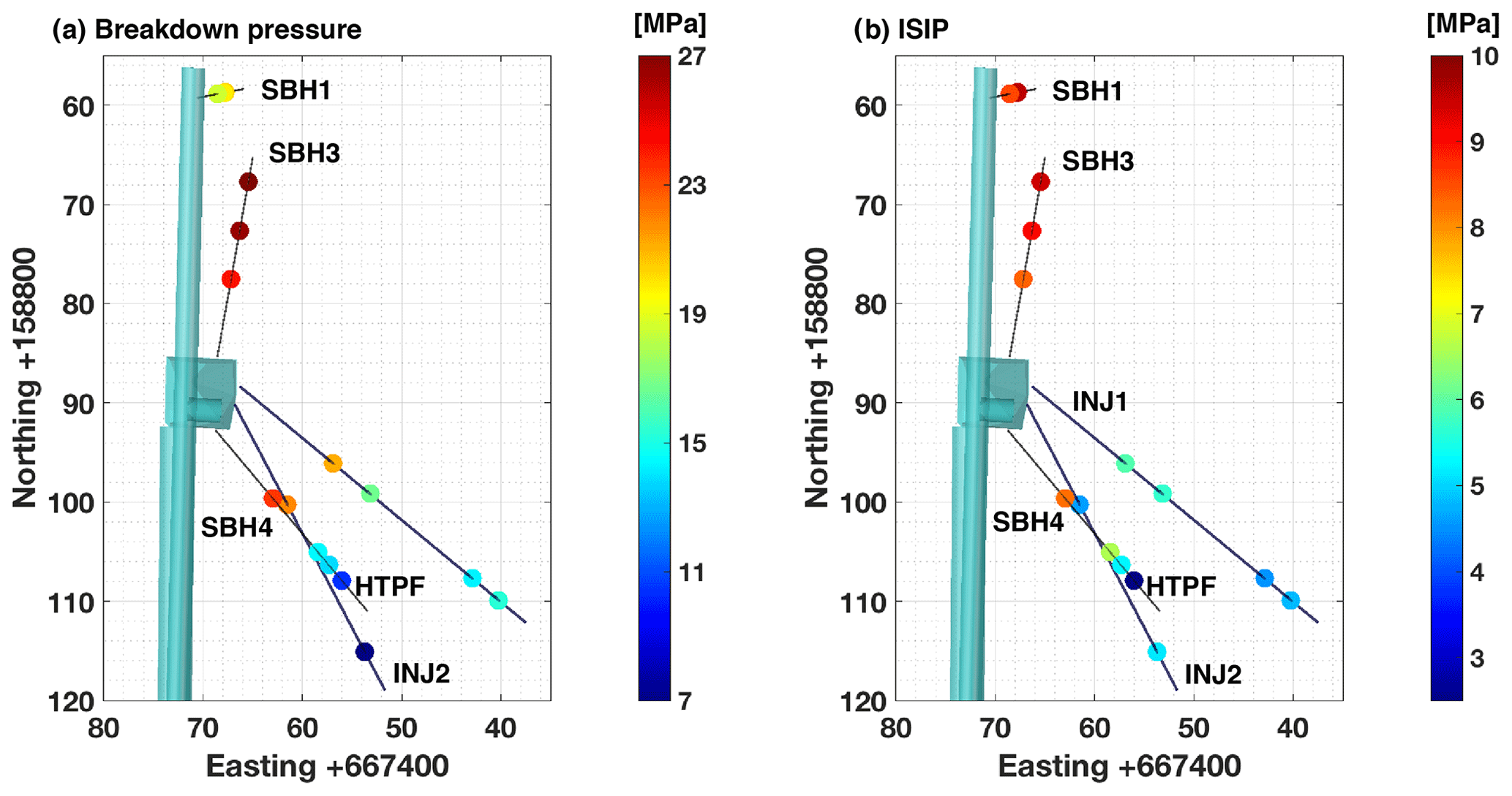
Figure 12Location of HF and MF experiments viewed towards west with a color code for (a) breakdown pressure and (b) instantaneous shut-in pressure (ISIP).
5.2 Fracture geometry
In the following, we compare the number of located seismic events between the HF and MF experiments. Then we compare the geophysical borehole loggings and impressions resulting in fracture traces at the wellbore, with the best-fitting planes through the microseismic clouds giving information on the fracture orientation away from the wellbores. One should be aware that the seismic monitoring array differed between the HF and MF experiments, which results in different network sensitivities and location accuracies. The number of located microseismic events for all HF experiments and minifracs during each frac–refrac (F–RF) cycle are presented in Fig. 13. All located events occurring during injection are indicated by colored bars, while the grey bars on top indicate the events after fluid injection (during shut-in and bleed-off time). The following key findings from Fig. 13 can be noted.
-
On average, the total number of located seismic events does not differ significantly between the MF and HF experiments, although the variability from experiment to experiment is large. This is somewhat surprising knowing that about 10 L was injected during the MF experiments and 1000 L during the HF experiments.
-
The variability of the number of seismic events is particularly obvious when comparing MF6, MF7, HF5, and HF6 (all experiments exhibit fewer than 50 events) with, for example, HF2 (531 events). Note that it cannot be ruled out that the different seismic network layouts for HF and MF affect the sensitivity towards detecting lower-magnitude events and can thus influence the result.
-
However, looking at frequency–magnitude distributions and the corresponding magnitude of completeness analyses presented by Villiger et al. (2019) suggests that for the HF injection experiments, not all the variability in detected and located seismic events can be attributed to sensitivity variations of the seismic network. A possible explanation for the low number of located events during MF6 and MF7 is the fact that they were close to the shear zone S3. During injection experiment HF5 a direct shortcut to a geophysical observation borehole was created. Injection experiment HF6 was executed at the wrong borehole interval, wherein a preexisting fracture was stimulated, which was already stimulated before during the hydraulic shearing (HS) experiment.
-
The minifracs show a tendency to have relatively more seismic events during shut-in (34.2 %) and bleed-off time compared to the hydraulic fracturing experiments (5.9 %).
-
During the MF experiments, typically a small number of events occur during the formation breakdown cycle (F) compared to the refrac (RF) cycles, except for MF4 and MF5. MF5 had an insufficient sealing of the experiment section, allowing the fluid to bypass the packer. Nevertheless, the seismic response is high and the experimental summary cards (Supplement) indicate that most of the seismic events are located around the borehole up to 4 m away from the injection point, with some minor events located 7 to 10 m away from the injection interval.
-
During the HF experiments, most seismicity occurs during the refrac cycles (RF) whereby the injected volume and the flow rate progressively increase. Except for experiment HF6, no seismicity was observed during the pressure-controlled step (SR) test. Prior to this experiment, we opened the valve of the injection interval to drain the fracture system. The small injection volume during the pressure-controlled step test and the small flow rates were not sufficient to reinitiate microseismic activity.
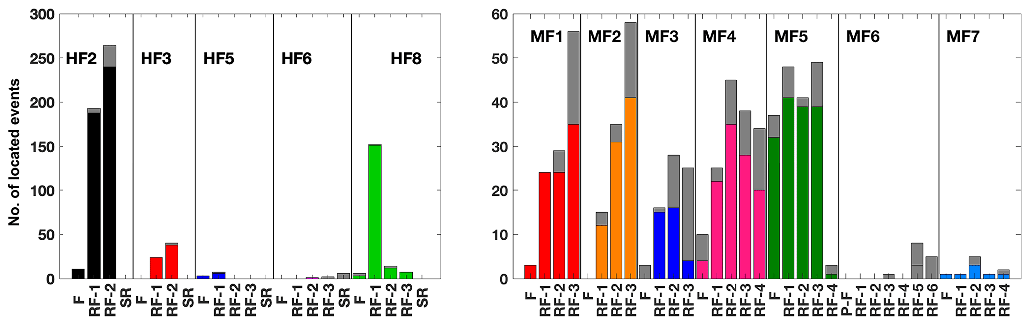
Figure 13The hydraulic fracturing (HF) and minifracs (MFs) from the stress characterization phase are presented in an event versus frac–refrac histogram. The color in the histograms corresponds to the number of events during injection. The grey bar on top of the histograms indicates the seismic events after injection shut-in.
The poles to the fracture traces determined at the borehole wall from acoustic televiewer data (see Fig. 6) in the boreholes INJ1 and INJ2 for the HF experiments are presented in Fig. 14a, and the pole to the fracture traces from the minifracs using impression packers are presented in Fig. 14b. We assume that these traces correspond to the fractures initiated during the frac cycle (formation breakdown). The fractures during HF experiments presented in Fig. 14a are subvertical with a N to NE dipping direction. The HF traces are axial or make a small angle to the injection borehole axes. The foliation orientation (337/15∘) is indicated by the magenta pole in Fig. 14, which also corresponds to the main brittle fracture set. The minifracs MF8–MF11 were executed in the subvertical borehole SBH1. The orientation of the minifracs (Fig. 14b) is primarily aligned with this foliation plane except for MF09 and MF10 that have a similar trace orientation to the HF experiments. The minifracs MF08 and MF11 orient towards the foliation and the brittle fracture orientation in the host rock (compare Fig. 2a) such that the fracture opened along the foliation. The orientation of fracture traces MF01 and MF02 from the subhorizontal borehole SBH3 shows a radial fracture initiation, which highlights the dominating control of foliation as such orientation is not the most favorable for initiation at the borehole from a stress concentration viewpoint.
The pole points from the plane fit to the seismic clouds are presented in Fig. 14c for the HF experiments and Fig. 14d for the minifracs. For both HF and MF, most of the seismic best-fit planes are subvertical, striking E–W and slightly dipping to the south. Note that some of the plane fits are poorly constrained due to the small number of located seismic events, i.e., HF3. Also, we noticed a change in orientation for HF2 with injected volume. During the first refrac cycle RF1, the seismic cloud orients itself vertically, striking ESE–WNW. Considering all seismic events including refrac cycle RF2, the seismic cloud orients itself subvertical, striking E–W similar to the minifracs. For experiment HF3, two different clusters are possible depending on the seismic events. The first fit indicates a subvertical plane striking towards S–N with a misfit of 1.2 m. The second cluster orients itself subvertical in E–W. The data presented in Fig. 14 are summarized in the Supplement (Sect. S5) with wellbore trace description and best plane fit details.
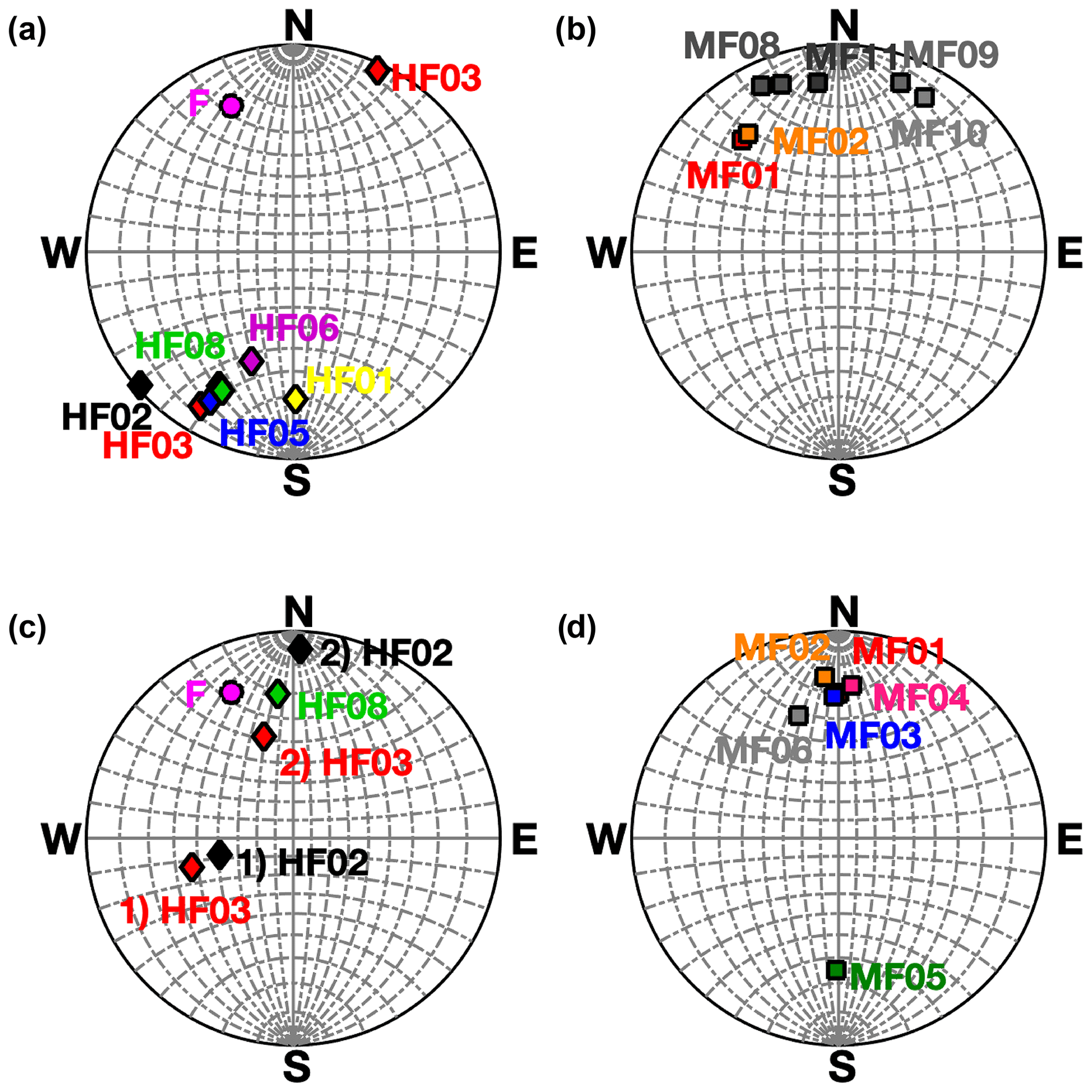
Figure 14The newly created fracture traces from geophysical borehole logging and impression packers are presented in a lower-hemisphere stereonet for the HF experiment (a) and the MF experiment (b). The pole points of the plane fits from the seismic events are indicated in a lower-hemisphere stereonet for both the HF experiment (c) and the MF experiment (d). The foliation is indicated by the magenta circle in panels (a) and (c). The color code is the same as for Fig. 13.
5.3 Fracture propagation
Fracture propagation during the fluid injection can be tracked using the seismic events that move away from the injection interval. In Fig. 15, all seismic events from the minifracs (MFs) are presented with grey circles. The grey circles are absent after 10 L of injected volume as it is the maximum injected volume for these experiments (Fig. 15). Further, the circle shows two localizations, one along the 10 m axis and the other with increasing injection volume starting at around 2 m for 0.3 L and ending at around 7 m for 10 L. The grey circles at 10 m are associated with the drained and disturbed stress field around the AU tunnel. On the other hand, the colored circles present the HF experiments. They show a positive correlation between distance and fluid injection. The distance stops increasing after an injection of 60 L and stays around 10 m. The injection of 1 m3 fluid into the fracture network results in observed seismic events maximally 20 m away from the injection interval, whereby the 10 L injected during the minifracs shows a maximum distance between the injection interval and the farthest event of 7 to 10 m.
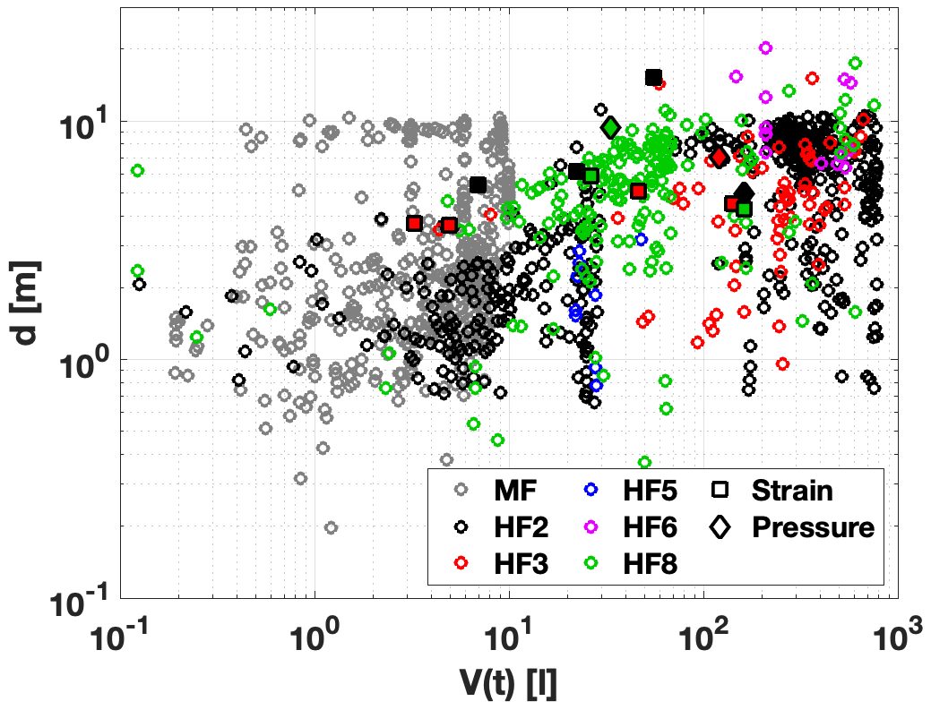
Figure 15The corrected injection volume including backflow correction is presented against the distance from the located seismic events to the midpoint of the injection location. The grey circles present all the located seismic events from the minifracs without subdividing them. The other circles present different HF experiments. The squares are tracked from FBG sensors or the distributed strain system (DSS), and the diamonds are taken from the transient pressure interval.
Instantaneous tensional strain and pressure response are tracked through our experiments to get the geometry of the hydraulic fractures. The midpoint of the strain or pressure sensor interval and the injection point is known, and the picked time is calculated for the corresponding corrected injection volume. The fracture distance of HF3 agrees between the strain and seismic observations for a small injection volume. With increasing injection volume, the seismic events propagate towards 10 m for an injection volume of 700 L. Two strain measurements indicate fracture opening 5 to 6 m away from the injection point and instantaneous pressure increases 7 m away for an injection volume of 50 to 105 L. For experiment HF8, the strain measurements at 30 L indicate a distance of 6 m from the injection point; the farthest seismic event is 7 m away from the injection interval. The pressure data point from experiment HF8 has a distance of ∼9 m and responds after 20 L of injection. At the same volume, the seismic cloud indicates a distance to injection of around 8 m. Considering the strain and pressure measurements from experiment HF2, we see that the distance of the seismic events is 2 times smaller compared to a strain sensor. It is remarkable that the seismic events are restricted to within 10 m of distance at high-pressure injection even though we know the hydraulic fracture is 15 m in length (HF2 strain sensor at 15 m). This agrees well with the observation of Warpinski et al. (2013) that the hydraulic fracture is essentially aseismic and that the stress-induced microseismicity is located at fractures with a significant dimension around the hydraulic fracture.
6.1 Hydraulic and mechanical response to hydraulic fracturing
Hydraulically, two different behaviors were observed in experiments performed south of S3 (HF3 and HF8) and north of the S3 (HF1, HF2, and HF6) shear zone. The differences consisted of lower pressure levels (fracture propagation, jacking, and ISIP), larger recovered water volumes, and larger final injectivity for experiments north of S3. Our proposed explanation for this behavior is as follows.
During the experiments performed south of S3, the newly initialized HF was only able to propagate a short distance in intact rock before it connected to the densely fractured S3 shear zone, which is bounded by two metabasic dykes, and therein two subnormal fracture systems are found. This highly transmissive structure is able to drain the injected fluid from the HF towards the AU tunnel. None of the HF experiments performed south of S3 were able to fracture through this geological structure. This is due to two reasons: (1) the structure's high transmissivity drains the fluids and prevents further pressure propagation, and (2) the stress variations in the structure's vicinity are not favorable for further fracture propagation. This is further supported by the small fluid recovery (less than 2 %) from the injection borehole for these injection tests, which suggests a strong hydraulic gradient forcing the injection fluid into the S3 shear zone and toward the AU tunnel.
The HF experiments north of S3 (HF1 and HF2) were able to initialize and propagate before leak-off dominated the natural fractures associated with the ductile shear zone S1. This less transmissive S1 shear zone can be described by a single fracture system in which one part of the fractures is capable of transporting fluid and the other part only stores the fluid (known as dead-end fractures). These tests are also more distant from the AU tunnel and thus in a volume isolated from its influence. Therefore, the observed fluid recovery from the injection location reaches values of 15.0 %–23.5 % for the first two refrac cycles. The HF6 experiment is comparable with HF1 and HF2 except for preexisting fractures influencing hydraulic fracturing initiation.
The tilt response reflects the hydraulic balance observations; i.e., the tilt magnitudes are smaller for the experiment south than north of S3. The FBG strain sensors show both tensional and compressional signals. High tensional signals are related to fracture pressurization and opening, reflecting hydraulic connections. In response to fracture opening, some other segment of the rock mass needs to compensate, and this is captured by the observed compressional signals. An example of such behavior is visible along FBS2 in Fig. 10f, with an increasingly compressive signal from 5 to 16 and from 40 to 26 m centered around a strongly tensional rock mass section at 20 m. The repartition of strain response is also influenced by the location of the injection south or north of S3. For the tests located south of S3, a tensional signal on the FBG sensors is predominantly observed in the S3 shear zone. The temporal evolution of the strain signal also suggests modifications of the flow path during the injections. Indeed, some sensors that initially react in compression later show an abrupt reversal toward tensional strain, indicating that they are now part of the active flow system. In turn, this influences previously active sections as sensors that were in tension stabilize or reverse, indicating a transfer of the flow portion towards the newly activated rock mass sections (Fig. 10).
For the injection locations north of S3, the geometry of our monitoring system implies that the distance between the injection points and the FBG sensors is comparatively larger. Therefore, smaller strain magnitudes are expected and observed.
6.2 Borehole trace and fracture tortuosity
The comparison of the fracture trace orientation at the borehole wall observed by acoustic televiewer logging with the orientation of the seismic cloud associated with a given fracture allows for the assessment of fracture rotation, also referred to as tortuosity, in the near field of the borehole (Bunger and Lecampion, 2017). An angular difference of about 30∘ is typical for most of our experiments. The inflating packers isolate the injection zone, and therefore the HFs initiate in the region controlled by near-wellbore stress concentration. This depends on the created fracture morphology and the orientation of the borehole with respect to the in situ stress state. This problem entirely relates to bigger uncertainty in determining the stress orientation from direct wellbore information using hydraulic fracturing. The minifracs indicate a bigger variability for the trace orientations than for the seismic cloud data (Fig. 14). These experiments were primarily performed in intact rock in two horizontal and one subvertical borehole and affected a small volume of intact rock around the borehole. For the HF experiments a larger amount of fluid was injected in a moderately fractured rock mass, and the flow rate was around 5 L min−1 during the frac cycle. The variability tends to be smaller for the HF traces using a higher flow rate, promoting dominant fluid pathways compared to a low flow rate (MF), which tends to have different fracture geometries in the near wellbore. The big flow rates and the test volume interacting with the hydraulic fracture will inevitably reach some significant features that affect the geometry of the seismic cloud, which has been confirmed by our experiments (more in the following section). The fracture traces observed at the borehole wall mostly extended below the packers. It is unclear if they initiated at the packer location or grew beyond them later during the successive propagation phase of the experiments.
6.3 Seismic response and fracture geometry
A key element to track fracture geometries beyond the borehole wall traces is microseismic event clouds. The spatial resolution of our seismic data does not permit the mapping of the near-well effect, but it does allow for the assessment of the fracture geometry at a scale >1 m. Strain response and pressure observations also permit to some extent the tracking of the geometry of hydraulic fractures. These data allow us to show that the geometry of the fractures departs strongly from the idealized radially growing penny-shaped or 2-D plain strain fractures. Instead, we observe fracture extension initially vertically downward, developing later along an E–W-oriented plane. The flow geometry is rather one-dimensional and pipe-like, likely formed by natural fracture intersections (Evans et al., 2005). In addition, during experiment HF2, multiple fractures at the early time of the injection were observed. Evidence for these early fractures not far apart from each other is given by two tensional signals in strain monitoring borehole FBS1 at a depth of 31.8 and 33.0 m (Fig. 10b).
Generally, this confirms the strong influence of preexisting fractures and fracture intersections on the structure of the hydraulic fracture propagation. It is furthermore noteworthy that the approximation of a penny-shaped fracture may not be appropriate in our case as the seismic clouds indicate a unidirectional instead of radial fracture growth (compare Fig. 8). Therefore, multiple fractures should be considered to advect the fluid rather than a single fracture. Considering the fracture geometry with two different orientations (HF2, HF3) a leak-off point may be estimated at which the fluid starts to follow the preexisting fracture network striking in the E–W direction. This leak-off point seems to be at a distance of 10 m from the injection point (Fig. 15). Further away from the injection point no seismic activity was observed. With ongoing hydraulic fracturing, more and more preexisting fractures will be connected, which results in an increase in swept volume and a decrease in fracture fluid pressure. This decreases the efficiency of creating new fractures, and therefore seismicity decreases until enough overpressure is created to shear along preexisting fractures or continue to grow tensile fractures. The interpretation agrees with the conceptual model for the HF experiment described as primary fracturing with shear stimulation leak-off by McClure and Horne (2014).
The maximal number of located seismic events from the HF experiment is 730, and the one from the minifracs is 646. However, seismic activity seems to be larger for the MF given the comparably smaller injection volume of 10 L compared to >1000 L for the HFs. Only experiments HF2 and HF8 reach a number above 100 located seismic events (Fig. 13). A possible reason may be stress relaxation from the HS experiments (Krietsch et al., 2019a) executed 5 months before the HF experiments. This would mean that shear relieved in the previously stimulated rock volume prevents new seismicity from occurring. However, it seems that the HF experiments have also been conducted in a stress field that is naturally different from the MF locations.
6.4 Permeability creation by HF
All the performed hydraulic fractures generated a transmissivity increase of about 3 orders of magnitude. This increase remains after the pressure is relieved and in this sense is permanent, i.e., is not related to the transient fracture opening under high-pressure injections. This indicates that the fractures never completely close back when the pressure is relieved. The final transmissivity matches one of an unstimulated fracture in our rock mass (Jalali et al., 2018a). The final transmissivity correlates positively with the final injectivity, which characterizes the newly created hydraulic fracture. Considering the injectivity value from the pressure-controlled step test has the advantage that it is directly related to the bulk mass compliance (rock mass compliance and fracture compliance) at a short timescale. In addition, we can characterize the liftoff (herein: jacking pressure) of the intersecting fracture and the injectivity after jacking in the injection interval. The drawback is that the flow is only at a quasi-steady state. For transmissivity values, we used constant head injection and pulse injection tests at low pressure (<0.6 MPa). This method is time-consuming and it does not account for mechanical effects but has the advantage of reaching steady-state conditions, which allows for a characterization of the bulk volume farther away than the pressure-controlled step test.
Hence, both methods are mandatory to understand the change in flow field and permeability. Considering an EGS system with an injection and a production interval, a certain injection pressure and probably a back pressure on the production interval is applied. Both injection and production intervals are able to change the hydromechanical parameters of the nearby fractures. Then the injectivity value is able to describe this interaction in which the transmissivity describes the overall bulk volume of the connected fracture network. In our experiment, all the newly created hydraulic fractures (except HF6) were mechanically closed after the reservoir was depressurized. Low-pressure constant head injection was insufficient to open the closed hydro-fracture. Thus, the newly created transmissivity is only linked to the new hydraulic fracture intersecting the wellbore. In terms of scaling we estimate transmissivity only on single wellbores, and no cross-hole tests were performed to estimate the new fracture network transmissivity. Therefore, the presented values of the final transmissivity are rather small.
6.5 Stress heterogeneity
For experiments executed south or north of S3 the ISIP stabilizes around 5 MPa and only deviates slightly. The jacking pressure is similar in magnitude compared to the ISIP for the experiments south of S3 (see Fig. 5). The situation differs for the experiments north of S3 as the magnitude of the jacking pressure is reduced. It reaches a value between 60 % and 80 % of ISIP. The similarity of jacking pressure and ISIP is a strong indication that they reflect the minimum principal stress magnitude, but further analysis is necessary to confirm that, which is not part of this publication.

Figure 16(a) Stereonet with a perturbed and unperturbed stress field as well as a Mohr–Coulomb diagram representing the perturbed (b) and unperturbed (c) stress field (including a hydrostatic pressure of 0.3 MPa) as Mohr circles. The failure limits assuming a friction coefficient of 0.6–0.8. Overpressure of 5 to 9 MPa is shown. The newly created hydraulic fractures from the ATV log (triangle) and the best-fit plane from the seismic profiles (squares) are presented with computed normal stress and shear stress. The color and symbol key in panel (b) are also applicable for panel (c). (d) The sketch indicates the change from the unperturbed (grey arrows on the outside) to perturbed stress field (black arrows inside) approaching the two different shear zones S1 and S3.
Approaching the shear zones S1 and S3 changes the stress observations significantly. For the HF experiments, it is best described by the perturbed stress field for small volumes of injection, i.e., the frac and first refrac cycle. Figure 16b shows the perturbed stress state as Mohr circles for the newly created hydraulic fractures from the ATV log (triangles) and the best-fit plane from seismicity (squares). Assuming higher perturbation during the breakdown cycle creating the new hydraulic fracture intersecting the borehole agrees well with the higher overpressure. Propagating the hydraulic fracture further away results in a decrease in the overpressure in the perturbed stress field (Fig. 16b) but an increase in the unperturbed one (Fig. 16c). Therefore, the unperturbed stress state cannot describe the behavior of the hydraulic fracture at the early time. The orientation of the seismic cloud is subhorizontal towards south considering all located seismic events (i.e., RF2). This reorientation of the fracture is controlled by the leak-off into the preexisting fracture network striking in E–W direction. Note that the density of preexisting fractures is increased approaching the S1 and S3 shear zones. At this point, the best estimate of the stress state can be described by the unperturbed stress field assuming smaller stress magnitudes. Figure 16d shows the situation in terms of the minor and major principal stress axis being reoriented approaching the shear zones. The perturbed stress field is a consequence of the preexisting fractures related to S1 and S3 and the scatter of the perturbed one. We assume that this reorientation of the fracture depends directly on the connectivity of the preexisting fracture network.
In this paper, the spatial and temporal evolution of rock deformation, transient fracture fluid pressure, and seismicity during six intermediate-scale hydraulic fracturing experiments are presented. One of the key findings of this work is that the fracturing processes are strongly influenced by site-specific characteristics, natural fractures, and local heterogeneities. This is to be expected in any rock mass since heterogeneities are always present in natural media. If the details of the observations presented in this paper are site specific, the overall processes and behavior are likely reproducible at any site, and we attempt to formulate these general behaviors in the following conclusions.
-
The heterogeneities lead to distinct behavior in terms of pressure responses and flow: tests performed north or south of the brittle–ductile shear zone S3 respond differently. We associate these differences principally with two effects. Firstly, the shear zones have impacted the stress state locally, and this in turn affects the fracture propagation. Secondly, the shear zones and the associated fracturing influence the flow in the experimental volume. When the hydraulic fracture grows, it connects and leaks into the preexisting fracture network, and thus at some point the energy required to create new fracture surfaces is not sufficient and tensile fracture stops. The flow is then largely dominated by the natural fracturing. In that regard, the brittle–ductile shear zone S3 acts as a main drain and constant pressure boundary, while connection to the S1 shear zone and associated fracturing provide larger storage possibilities.
-
The deformation field associated with fracture growth is complex, showing local extension on the fracture path that is compensated for by compression in the surrounding rock mass. Such a deformation pattern is strongly coupled to the pressure field variations associated with the injections.
-
The creation of new fractures at the borehole is clearly visible on borehole wall acoustic images. The orientation of the fracture traces, however, is variable and does not provide a good estimation of the independently measured far-field stress orientation. The variability of the fracture trace could be explained by rock strength anisotropy (Dutler et al., 2018). It could also be influenced by packer stresses or local stress heterogeneities induced by natural fractures, as we observed that the new fracture trace extends below the packer and often abuts natural fractures. Our data set does not allow us to determine if the fractures initiate below the packers or in the injection interval, although since the packer pressure is always maintained above the interval pressure to ensure sealing, the former is not unlikely.
-
The growth of the hydraulic fractures is strongly influenced by natural fractures. This leads to complex geometry departing from theoretical mode I fracture geometries. Our data highlight the simultaneous growth of parallel fracture strands. They also suggest channelized growth (pipe-like geometry) instead of planar growth.
-
The number of seismic events associated with each fracture treatment varies a lot. This is not related to the injected volume but seems to be influenced by heterogeneities in stress and flow with our experimental volume.
-
A significant increase in transmissivity of 2–4 orders of magnitude from well tests before and after HF was observed. The final transmissivity correlates positively with the final injectivity obtained from the pressure-controlled step tests. Such a permanent permeability increase is not consistent with pure mode I fractures in homogenous media that would close back after depressurization. The heterogeneities and associated complexity of the hydraulic fractures probably favor the permanent transmissivity gain. The final transmissivities are comparable with the unstimulated natural fractures in our rock mass (Jalali et al., 2018b), which supports the conclusion that connectivity to the natural fracture system controls the final transmissivities.
-
Despite the complexity of the local fracturing processes, the spatial distribution of microseismic events associated with fracture growth seems to be predominantly controlled by the stress state. In that regard, we observe rotations related to stress perturbations that have been highlighted within our experimental volume (Krietsch et al., 2019b). A comparison of deformation and pressure monitoring within the rock mass and the location of microseismic events suggests that the activation of seismic events lags slightly behind the propagation of the pressure front. This suggests that the treatment size estimated by microseismic mapping could underestimate the actual rock volume affected by hydraulic fracturing processes.
The Grimsel ISC Experiment Description is available at https://doi.org/10.3929/ethz-b-000310581 (Doetsch et al., 2018a) and the hydromechanical data set from the Grimsel ISC hydraulic fracturing experiment is available at https://doi.org/10.3929/ethz-b-000328270 (Dutler et al., 2019). The data from the minifrac experiments are available at https://doi.org/10.3929/ethz-b-000217536 (Gischig et al., 2018).
The supplement related to this article is available online at: https://doi.org/10.5194/se-10-1877-2019-supplement.
The monitoring setup was designed by VG, JD, MJ, and FA. The injection protocol and operation planning were designed by ND and BV. All the authors were part of the data acquisition team during the HF experiments of the ISC project; FA was the project administrator. The formal analysis, data curation, and data visualization, including writing the original draft, were done by ND with the help of BV. The writing review and editing were done by VG, LV, HK, JD, BB, MJ, and FA. The supervision and funding acquisition for this work were done by BV.
The authors declare that they have no conflict of interest.
The ISC is a project of the Deep Underground Laboratory at ETH Zurich established by the Swiss Competence Center for Energy Research – Supply of Electricity (SCCER-SoE) with the support of Innosuisse. Funding for the ISC project was provided by the ETH Foundation with grants from Shell, EWZ, and the Swiss Federal Office of Energy through a P&D grant. We thank Gerd Klee and his staff from MeSy Solexperts, Bochum (Germany), for their good collaboration and helpful discussions. The Grimsel Test Site is operated by NAGRA, the National Cooperative for the Disposal of Radioactive Waste. We are indebted to NAGRA for hosting the ISC experiment in their GTS facility and to the NAGRA technical staff for on-site support.
This research has been supported by the Schweizerischer Nationalfonds zur Förderung der Wissenschaftlichen Forschung (grant nos. 200021_165677 (Nathan Dutler) and 200021_169178 (Hannes Krietsch)) and the Eidgenössische Technische Hochschule Zürich (grant no. ETH-35 16-1 (Linus Villiger)).
This paper was edited by Federico Rossetti and reviewed by David McNamara and one anonymous referee.
Amadei, B. and Stephansson, O.: Rock Stress and Its Measurements, Springer International Publishing AG, ISBN 978-94-011-5346-1, 1997. a
Amann, F., Gischig, V., Evans, K., Doetsch, J., Jalali, R., Valley, B., Krietsch, H., Dutler, N., Villiger, L., Brixel, B., Klepikova, M., Kittilä, A., Madonna, C., Wiemer, S., Saar, M. O., Loew, S., Driesner, T., Maurer, H., and Giardini, D.: The seismo-hydromechanical behavior during deep geothermal reservoir stimulations: open questions tackled in a decameter-scale in situ stimulation experiment, Solid Earth, 9, 115–137, https://doi.org/10.5194/se-9-115-2018, 2018. a
Barton, C. A., Zoback, M. D., and Moos, D.: Fluid flow along potentially active faults in crystalline rock, Geology, 23, 683–686, 1995. a
Bredehoeft, J. D., Wolf, R. G., Keys, W. S., and Shutter, E.: Hydraulic fracturing to determine regional in situ stress filed, in the Piceance Basin, Colorado, Geol. Soc. Am. Bull., 87, 250–258, 1976. a, b
Brixel, B., Klepikova, M., Jalali, M., Roques, C., Lei, Q., Krietsch, H., and Loew, S.: Tracking fluid flow in shallow crustal fault zones: 1. New in situ permeability measurements, AGU Solid Earth, in review, 2019. a, b, c
Brown, D. W., Duchane, D. V., Heiken, G., Hriscu, V. T., and Kron, A.: Mining the earth's heat: Hot dry rock geothermal energy, Springer, https://doi.org/10.1007/978-3-540-68910-2, 2012. a, b
Bunger, A. and Lecampion, B.: Four Critical Issues for Successful Hydraulic Fracturing Applications, Rock Mechanics and Engineering, Vol. 5, chap. 16, CRC Press, Balkema, 2017. a
Doe, T. W. and Korbin, G. E.: A Comparison Of Hydraulic Fracturing And Hydraulic Jacking Stress Measurements, The 28th U.S. Symposium on Rock Mechanics (USRMS), 29 June–1 July 1987, Tucson, 283–290, 1987. a, b
Doetsch, J., Gischig, V., Krietsch, H., Villiger, L., Amann, F., Dutler, N., Jalali, R., Brixel, B., Giertzuch, P., Maurer, H., Wiemer, S., Loew, S., Saar, M., and Giardini, D.: Grimsel ISC Experiment Description, Tech. Rep. December, SCCER-SoE, ETH Zurich, Zurich, https://doi.org/10.3929/ethz-b-000310581, 2018a. a, b
Doetsch, J., Gischig, V., Villiger, L., Krietsch, H., Nejati, M., Amann, F., Jalali, M., Madonna, C., Maurer, H., Wiemer, S., Driesner, T., and Giardini, D.: Subsurface fluid pressure and rock deformation monitoring using seismic velocity observations, Geophys. Res. Lett., 45, 10389–10397, https://doi.org/10.1029/2018GL079009, 2018b. a
Dresen, G., Renner, J., Bohnhoff, M., Konietzky, H., Kwiatek, G., Plenkers, K., Klee, G., and Backers, T.: STIMTEC – a mine-back experiment in the Reiche Zeche underground, Geophys. Res. Abstr., EGU2019-9357, EGU General Assembly 2019, Vienna, Austria, 2019. a
Dutler, N., Nejati, M., Valley, B., Amann, F., and Molinari, G.: On the link between fracture toughness, tensile strength, and fracture process zone in anisotropic rocks, Eng. Fract. Mech., 201, 56–79, https://doi.org/10.1016/j.engfracmech.2018.08.017, 2018. a, b
Dutler, N., Gischig, V., Doetsch, J., Jalali, M., Krietsch, H., and Amann, F.: Hydro mechanical data set from the six Grimsel ISC hydraulic fracturing experiments, https://doi.org/10.3929/ethz-b-000328270, 2019. a
Economides, M. and Nolte, K.: Reservoir Stimulation, May, Wiley, Chichester, https://doi.org/10.1017/CBO9781107415324.004, 2000. a, b
Ellsworth, W. L.: Injection-Induced Earthquakes, Science, 341, 1225942, https://doi.org/10.1126/science.1225942, 2013. a
Evans, K. F. and Meier, P. M.: Hydrojacking and hydrofracturing tests in a fissile schist in South-west Switzerland: In-situ stress characterisation in difficult rock, edited by: Rossmanith, H. P., Proc. 2nd Int. Conf. on the Mechanics of Jointed and Faulted Rock, Vienna, 1995. a
Evans, K. F., Moriya, H., Niitsuma, H., Jones, R. H., Phillips, W. S., Genter, A., Sausse, J., Jung, R., and Baria, R.: Microseismicity and permeability enhancement of hydrogeologic structures during massive fluid injections into granite at 3 km depth at the Soultz HDR site, Geophys. J. Int., 160, 388–412, https://doi.org/10.1111/j.1365-246X.2004.02474.x, 2005. a, b
Evans, K. F., Zappone, A., Kraft, T., Deichmann, N., and Moia, F.: A survey of the induced seismic responses to fluid injection in geothermal and CO2 reservoirs in Europe, Geothermics, 41, 30–54, https://doi.org/10.1016/j.geothermics.2011.08.002, 2012. a
Evans, K. F., Wieland, U., Wiemer, S., and Giardini, D.: Deep Geothermal Energy R&D Roadmap for Switzerland, 2014, Tech. rep., Swiss Competence Center for Energy Research – Supply of Electricity, https://doi.org/10.3390/en7074397, 2014. a
Gischig, V. S., Doetsch, J., Maurer, H., Krietsch, H., Amann, F., Evans, K. F., Nejati, M., Jalali, M., Valley, B., Obermann, A. C., Wiemer, S., and Giardini, D.: On the link between stress field and small-scale hydraulic fracture growth in anisotropic rock derived from microseismicity, Solid Earth, 9, 39–61, https://doi.org/10.5194/se-9-39-2018, 2018 (data available at: https://doi.org/10.3929/ethz-b-000217536). a, b, c
Haimson, B. C. and Cornet, F. H.: ISRM suggested methods for rock stress estimation part 3: Hydraulic fracturing (HF) and/or hydraulic testing of pre-existing fractures (HTPF), Int. J. Rock Mech. Min., 40, 1011–1020, https://doi.org/10.1016/j.ijrmms.2003.08.002, 2003. a, b
Häring, M. O., Schanz, U., Ladner, F., and Dyer, B. C.: Characterisation of the Basel 1 enhanced geothermal system, Geothermics, 37, 469–495, https://doi.org/10.1016/j.geothermics.2008.06.002, 2008. a
Hertrich, M. and Maurer, H.: Understanding Deep Geothermal Reservoirs: A journey from laboratory-scale experiments to investigations at realistic scales, Newsletter of the NEAR-SURFACE GEOPHYSICS Technical Section of The Society of Exploration Geophysicists, 26, Q1, available at: https://seg.org/Portals/0/SEG/News and Resources/Near Surface/Near Surface Newsletter/2011-present/2019_Q1.pdf (last access: 31 October 2019), 2019. a
Hubbert, M. K. and Willis, D. G.: Mechanics of hydraulic fracturing, Transactions of the american institute of mining and metallurgical engineers, Petroleum Transactions, AIME, 210, 153–163, 1957. a, b
Jacob, C. E. and Lohman, S. W.: Nonsteady flow to a well of constant drawdown in an extensive aquifer, EOS T. Am. Geophys. Un., 33, 559, https://doi.org/10.1029/TR033i004p00559, 1952. a
Jalali, M., Gischig, V., Doetsch, J., Näf, R., Krietsch, H., Klepikova, M., Amann, F., and Giardini, D.: Transmissivity Changes and Microseismicity Induced by Small-scale Hydraulic Fracturing Tests in Crystalline Rock, Geophys. Res. Lett., 45, 2265–2273, https://doi.org/10.1002/2017GL076781, 2018a. a
Jalali, M., Klepikova, M., Doetsch, J., Krietsch, H., Brixel, B., Dutler, N. O., Gischig, V. S., and Amann, F.: A Multi-Scale Approach to Identify and Characterize the Preferential Flow Paths of a Fractured Crystalline Rock, in: 2nd International DFNE Conference, p. 0734, Seattle, 2018b. a, b, c, d
Jeffrey, R. G., Bunger, A., Lecampion, B., Zhang, X., Chen, Z., van As, A., Allison, D., de Beer, W., Dudley, J., Siebrits, E., Thiercelin, M., and Mainguy, M.: Measuring Hydraulic Fracture Growth in Naturally Fractured Rock, SPE Annual Technical Conference and Exhibition, 4–7 October 2009, New Orleans, Louisiana, 1–19, https://doi.org/10.2118/124919-MS, 2009. a, b
Jeffrey, R. G., Chen, Z., Mills, K., and Pegg, S.: Monitoring and Measuring Hydraulic Fracturing Growth During Preconditioning of a Roof Rock over a Coal Longwall Panel, in: Effective and Sustainable Hydraulic Fracturing, InTech, Vol. 45, 893–914, https://doi.org/10.5772/56325, 2013. a
Keusen, H. R., Ganguin, J., Schuler, P., and Buletti, M.: Geologie, Tech. Rep. NTB87-14, Nagra, Wettingen, 1989. a
Kneafsey, T., Dobson, P., Ajo-Franklin, J., Valladao, C., Blankenship, D., Knox, H., Schwering, P., Morris, J., Smith, M., White, M., Johnson, T., Podgorney, R., Mattson, E., Neupane, G., Roggenthen, W., and Doe, T.: The EGS Collab Project: Stimulation and Simulation, ARMA2018–1345, American Rock Mechanics Association, Seattle, 2018. a
Krietsch, H., Doetsch, J., Dutler, N., Jalali, M., Gischig, V., Loew, S., and Amann, F.: Comprehensive geological dataset describing a crystalline rock mass for hydraulic stimulation experiments, Scientific Data, 5, 180269, https://doi.org/10.1038/sdata.2018.269, 2018. a
Krietsch, H., Löw, S., Gischig, V., Amann, F., and Renner, J.: Hydro-Mechanical Responses of a Fractured Rock Mass during Decameter-Scale Hydraulic Stimulation Experiments, ETH Zürich, https://doi.org/10.3929/ethz-b-000372209, 2019. a, b, c
Krietsch, H., Gischig, V., Evans, K., Doetsch, J., Dutler, N. O., Valley, B., and Amann, F.: Stress Measurements for an In Situ Stimulation Experiment in Crystalline Rock: Integration of Induced Seismicity, Stress Relief and Hydraulic Methods, Rock Mech. Rock Eng., 52, 517–542, https://doi.org/10.1007/s00603-018-1597-8, 2019b. a, b, c, d
Lister, J. R. and Kerr, R. C.: Fluid-mechanical models of crack propagation and their application to magma transport in dykes, J. Geophys. Res., 96, 10049, https://doi.org/10.1029/91JB00600, 1991. a
López-Comino, J. A., Cesca, S., Heimann, S., Grigoli, F., Milkereit, C., Dahm, T., and Zang, A.: Characterization of Hydraulic Fractures Growth During the Äspö Hard Rock Laboratory Experiment (Sweden), Rock Mech. Rock Eng., 50, 2985–3001, https://doi.org/10.1007/s00603-017-1285-0, 2017. a
Louis, C., Dessenne, J., and Feuga, B.: Interaction between water flow phenomena and themechanical behavior of soil or rock masses, in: Finite Elements in Geomechanics, edited by: Gudehus, G., 479–511, John Wiley & Sons, New York, 1977. a
Majer, E. L. and Doe, T. W.: Studying hydrofractures by high frequency seismic monitoring, Int. J. Rock Mech. Min., 23, 185–199, https://doi.org/10.1016/0148-9062(86)90965-4, 1986. a
Manning, C. E. and Ingebritsen, S. E.: Permeability Implications of the Continental of Geothermal Data Crust and Metamorphic Systems, Rev. Geophys., 37, 127–150, 1999. a
Martínez-Garzón, P., Bohnhoff, M., Kwiatek, G., and Dresen, G.: Stress tensor changes related to fluid injection at the Geysers geothermal field, California, Geophys. Res. Lett., 40, 2596–2601, https://doi.org/10.1002/grl.50438, 2013. a
Maxwell, S., Rutledge, J., Jones, R., and Fehler, M.: Petroleum reservoir characterization using downhole microseismic monitoring, Geophysics, 75, 75A129–75A137, https://doi.org/10.1190/1.3477966, 2010. a
McClure, M. W. and Horne, R. N.: An investigation of stimulation mechanisms in Enhanced Geothermal Systems, Int. J. Rock Mech. Min., 72, 242–260, https://doi.org/10.1016/j.ijrmms.2014.07.011, 2014. a, b
McGarr, A.: Maximum magnitude earthquakes induced by fluid injection, J. Geophys. Res.-Sol. Ea., 119, 1008–1019, https://doi.org/10.1002/2013JB010597, 2014. a
Meier, P. M., Rodríguez, A., and Bethmann, F.: Lessons Learned from Basel: New EGS Projects in Switzerland Using Multistage Stimulation and a Probabilistic Traffic Light System for the Reduction of Seismic Risk, Proceedings World Geothermal Congress, 19–25, available at: https://pangea.stanford.edu/ERE/db/WGC/papers/WGC/2015/31023.pdf (last access: 31 October 2019), 2015. a
Niitsuma, H., Fehler, M., Jones, R., Wilson, S., Albright, J., Green, A., Baria, R., Hayashi, K., Kaieda, H., Tezuka, K., Jupe, A., Wallroth, T., Cornet, F., Asanuma, H., Moriya, H., Nagano, K., Phillips, W. S., Rutledge, J., House, L., Beauce, A., Alde, D., and Aster, R.: Current status of seismic and borehole measurements for HDR/HWR development, Geothermics, 28, 475–490, https://doi.org/10.1016/S0375-6505(99)00024-3, 1999. a
Nolen-Hoeksema, R. C. and Ruff, L. J.: Moment tensor inversion of microseisms from the B-sand propped hydrofracture, M-site, Colorado, Tectonophysics, 336, 163–181, https://doi.org/10.1016/S0040-1951(01)00100-7, 2001. a
Roberts, R.: nSIGHTS Version 2.41a User Manual, available at: https://github.com/nsights/nSIGHTS/blob/master/documents/nSIGHTS_Users_Manual_V2.41a.pdf, (last access: 31 October 2019) 2006. a
Rubin, A. M.: Propagation of Magma-Filled Cracks, Annu. Rev. Earth Pl. Sc., 23, 287–336, https://doi.org/10.1146/annurev.ea.23.050195.001443, 1995. a
Rutledge, J. T., Phillips, W., and Mayerhofer, M.: Faulting Induced by Forced Fluid Injection and Fluid Flow Forced by Faulting: An Interpretation of Hydraulic-Fracture Microseismicity, Carthage Cotton Valley Gas Field, Texas, B. Seismol. Soc. Am., 94, 1817–1830, https://doi.org/10.1785/012003257, 2004. a, b
Rutqvist, J.: Determination of hydraulic normal stiffness of fractures in hard rock from well testing, Int. J. Rock Mech. Min., 32, 513–523, https://doi.org/10.1016/0148-9062(95)00039-J, 1995. a
Rutqvist, J. and Stephansson, O.: A cyclic hydraulic jacking test to determine the in situ stress normal to a fracture, Int. J. Rock Mech. Min., 33, 695–711, https://doi.org/10.1016/0148-9062(96)00013-7, 1996. a
Rutqvist, J. and Stephansson, O.: The role of hydromechanical coupling in fractured rock engineering, Hydrogeol. J., 11, 7–40, https://doi.org/10.1007/s10040-002-0241-5, 2003. a
Rutqvist, J., Noorishad, J., Tsang, C.-F., and Stephansson, O.: Determination of fracture storativity in hard rocks using high-pressure injection testing, Water Resour. Res., 34, 2551–2560, 1998. a
Spence, D. A. and Sharp, P.: Self-similar solutions for elastodynamic cavity flow, Proc. R. Soc. Lon. Ser.-A, 400, 289–313, 1985. a
van As, A. and Jeffrey, R. G.: Caving Induced by Hydraulic Fracturing at Northparkes Mines, Pacific Rocks, 2000, 353–360, 2000. a
Villiger, L., Gischig, V. S., Doetsch, J., Krietsch, H., Dutler, N. O., Jalali, M., Valley, B., Selvadurai, P. A., Mignan, A., Plenkers, K., Giardini, D., Amann, F., and Wiemer, S.: Influence of reservoir geology on seismic response during decameter scale hydraulic stimulations in crystalline rock, Solid Earth Discuss., https://doi.org/10.5194/se-2019-159, in review, 2019. a, b, c, d
Warpinski, N. R.: Measurement of width and pressure in a propagating hydraulic fracture, Soc. Petrol. Eng. J., 25, 46–54, 1985. a, b
Warpinski, N. R. and Branagan, P. T.: Altered-Stress Fracturing, J. Petrol. Technol., SPE-17533-PA, 41, 990–997, https://doi.org/10.2118/17533-PA, 1989. a
Warpinski, N. R., Mayerhofer, M. J., and Agarwal, K.: Hydraulic Fracture Geomechanics and Microseismic Source Mechanisms, SPE J., 18, 766–780, https://doi.org/10.2118/158935-PA, 2013. a, b
Warren, W. E. and Smith, C. W.: In situ stress estimates from hydraulic fracturing and direct observation of crack orientation, J. Geophys. Res., 90, 6829, https://doi.org/10.1029/JB090iB08p06829, 1985. a
Wenning, Q. C., Madonna, C., de Haller, A., and Burg, J.-P.: Permeability and seismic velocity anisotropy across a ductile–brittle fault zone in crystalline rock, Solid Earth, 9, 683–698, https://doi.org/10.5194/se-9-683-2018, 2018. a
Zang, A., Stephansson, O., Stenberg, L., Plenkers, K., Specht, S., Milkereit, C., Schill, E., Kwiatek, G., Dresen, G., Zimmermann, G., Dahm, T., and Weber, M.: Hydraulic fracture monitoring in hard rock at 410 m depth with an advanced fluid-injection protocol and extensive sensor array, Geophys. J. Int., 208, 790–813, https://doi.org/10.1093/gji/ggw430, 2016. a
Zimmermann, G., Zang, A., Stephansson, O., Klee, G., and Semiková, H.: Permeability Enhancement and Fracture Development of Hydraulic In Situ Experiments in the Äspö Hard Rock Laboratory, Sweden, Rock Mech. Rock Eng., 52, 495–515, https://doi.org/10.1007/s00603-018-1499-9, 2019. a
- Abstract
- Introduction
- Site and rock mass characterization
- Field setup and monitoring
- Overview of the HF experiments
- Comparison between stress characterization and HF experiments
- Discussion
- Conclusions
- Data availability
- Author contributions
- Competing interests
- Acknowledgements
- Financial support
- Review statement
- References
- Supplement