On the morphology and amplitude of 2D and 3D thermal anomalies induced by buoyancy-driven flow within and around fault zones

In the first kilometers of the subsurface, temperature anomalies due to heat conduction processes rarely exceed 20–30 ^∘C. When fault zones are sufficiently permeable, fluid flow may lead to much larger thermal anomalies, as evidenced by the emergence of thermal springs or by fault-related geothermal reservoirs. Hydrothermal convection triggered by buoyancy effects creates thermal anomalies whose morphology and amplitude are not well known, especially when depth- and time-dependent permeability is considered. Exploitation of shallow thermal anomalies for heat and power production partly depends on the volume and temperature of the hydrothermal reservoir. This study presents a non-exhaustive numerical investigation of fluid flow models within and around simplified fault zones, wherein realistic fluid and rock properties are accounted for, as are appropriate boundary conditions. 2D simplified models point out relevant physical mechanisms for geological problems, such as “thermal inheritance” or pulsating plumes. When permeability is increased, the classic “finger-like” upwellings evolve towards a “bulb-like” geometry, resulting in a large volume of hot fluid at shallow depth. In simplified 3D models wherein the fault zone dip angle and fault zone thickness are varied, the anomalously hot reservoir exhibits a kilometer-sized “hot air balloon” morphology or, when permeability is depth-dependent, a “funnel-shaped” geometry. For thick faults, the number of thermal anomalies increases but not the amplitude. The largest amplitude (up to 80–90 ^∘C) is obtained for vertical fault zones. At the top of a vertical, 100 m wide fault zone, temperature anomalies greater than 30 ^∘C may extend laterally over more than 1 km from the fault boundary. These preliminary results should motivate further geothermal investigations of more elaborated models wherein topography and fault intersections would be accounted for.

1 Introduction

In the shallow crust, several geological systems meet the necessary conditions for the occurrence of significant deep fluid circulation. Tectonically active systems, ash-flow calderas, sedimentary basins, and especially crustal fault zones correspond to dynamic systems that are sufficiently porous and permeable to host fluid circulation (e.g., Simms and Garven, 2004; Hutnak et al., 2009; Lopez et al., 2016; Patterson et al., 2018a; Duwiquet et al., 2019). As soon as rock permeability is large enough, meteoric, metamorphic, or magmatic fluids can flow along kilometer-scale pathways at velocities reaching up to several meters per year (e.g., Forster and Smith, 1989; López and Smith, 1995). When fluid velocity is sufficiently large, heat can be advected with the fluid to shallow crustal levels (e.g., Ague, 2014), leading to the development of hydrothermal reservoirs and thus to exploitable thermal anomalies. Similarly, when cold fluid is transferred to deep levels (or when deep hot fluids rise in the intermediate crust), precipitation of minerals can be favored and mineralizing processes may form exploitable ore deposits (e.g., Fehn et al., 1978; Boiron et al., 2003; Weis et al., 2012). Whether geothermal resources or mineral resources are targeted, the main questions that generally have to be addressed deal with the location and volume of the reservoir. This study is focused on the “geothermal side” of hydrothermal resources (i.e., mineralizing processes are not considered), particularly on the formation of anomalously hot and shallow hydrothermal reservoirs.

In shallow permeable zones, at the scale of kilometer-sized reservoirs, two main processes can control fluid circulation: (i) significant pressure gradients, which can result from topography or from magmatic or metamorphic fluid production; and (ii) buoyancy effects due to temperature-dependent fluid density that can result in thermal convection in permeable media. In the first case, the term “forced convection” is employed, while in the second case, “free convection” is used. Although both processes can occur at the same time (see, for example, the numerical models of the Basin and Range extensional geothermal systems by McKenna and Blackwell, 2000), one of the two convection modes may predominate. For example, in the case of significant topography (1000–2000 m), forced convection may control the fluid flow regime as in the case of Alpine hydrothermal systems (e.g., Sonney and Vuataz, 2009). However, in the case of a fault zone with a high permeability, free (thermal) convection may prevail over forced convection.

The possibility for thermal convection to occur within a permeable medium was often tested with the calculation of the Rayleigh number (e.g., Turcotte and Schubert, 2002). This dimensionless number depends on the imposed temperature gradient, the considered geometry, and fluid and rock properties. If the Rayleigh number exceeds a critical value, then thermal convection occurs. The critical value of 4π² (Lapwood, 1948) was determined by linear stability analysis for an infinitely long homogeneous porous medium, whereby fixed temperature conditions are applied on both horizontal boundaries, and for a constant viscosity fluid. For different (and more realistic) boundary conditions (e.g., fixed heat flow at depth and fixed pressure at the surface) the critical Rayleigh number is decreased (see Jaupart and Mareschal, 2011). When temperature-dependent viscosity is accounted for, Lin et al. (2003) demonstrated that the critical Rayleigh number is also decreased when compared to the constant viscosity case. In other words, when realistic boundary conditions are considered and when appropriate fluid properties are taken into account, the critical permeability for which free convection would occur is not as high as previously thought.

In the case of a finite-sized vertical fault zone, Malkovski and Magri (2016) developed a new linear stability analysis accounting for temperature-dependent fluid viscosity. They showed, in accordance with Wang et al. (1987), that the critical Rayleigh number can be expressed with the fault aspect ratio (half-width over depth) but also with a dimensionless thermal parameter describing the temperature dependence of the fluid viscosity. One of their conclusions is that the Rayleigh theory may not be sufficient when fluid properties are adequately considered. In addition, the critical permeability for which free convection develops may be 4 times lower than initially predicted within the constant viscosity hypothesis. One limit of their theoretical study lies, however, in the investigated temperature range, limited to a domain in which a linear fit to density variation holds. Indeed, for temperatures greater than 300 ^∘C, the linear fit no longer holds, and one must thus refer to a numerical approach whereby an appropriate density law (nonlinear, pressure- and temperature-dependent) can be accounted for.

In this study, we focus on hydrothermal convection that could lead to the establishment of exploitable thermal anomalies. Geothermal resources leading to power production generally require temperatures higher than 150 ^∘C, and present-day exploration projects tend to target supercritical conditions involving much higher temperatures (high-enthalpy geothermal systems or, as recently suggested, superhot geothermal systems; e.g., Scott et al., 2015; Watanabe et al., 2019), in particular around the brittle–ductile transition (350–400 ^∘C; Violay et al., 2017). It is thus necessary to study hydrothermal convection wherein temperature can exceed 300 ^∘C, a domain for which fluid properties are highly nonlinear. For example, Jupp and Schultz (2000) demonstrated that the surprising constant temperature of black smokers (around 380 ^∘C) could be explained by the maximization of the “fluxibility” parameter, which depends on thermodynamic properties of water (density, viscosity, and specific enthalpy).

Besides accounting for appropriate fluid properties, studies on hydrothermal convection need to consider realistic rock permeability. This physical property, initially supposed to be “static”, has increasingly been considered to be “dynamic”, not only through field and petrologic observations (e.g., Jamtveit et al., 2009; Faulkner et al., 2010; Stober and Bucher, 2015) but also in numerical models and laboratory experiments (Tenthorey and Cox, 2003; Tenthorey and Fitzgerald, 2006; Coelho et al., 2015; Ingebritsen and Gleeson, 2015; Mezri et al., 2015; Weis, 2015; Launay et al., 2019). Several mechanisms can explain the spatial (e.g., depth-dependent) and temporal (e.g., stress-dependent) variations of permeability. For example, fluid–rock interactions may involve mineralogical transformations leading to a continuous increase in permeability (Launay, 2018). A gradual permeability increase in a fault damage zone has been suggested by Louis et al. (2019) to explain the temporal evolution of the Beowawe hydrothermal system in Nevada. However, depending on the hydrogeologic and tectonic setting, a sudden increase or decrease in permeability could also happen and should significantly affect the fluid flow conditions. Whereas the effect of heterogeneous and dynamic permeability has already been studied around magmatic intrusions (e.g., Gerdes et al., 1998; Weis et al., 2012; Scott and Driesner, 2018; Launay, 2018), this is not the case for fault zones.

This study is intended to show, with a numerical modeling approach, how hydrothermal convection establishes in a permeable fault zone, how convective patterns are organized, and what kind of particular phenomena can be observed. The effects of topography are not accounted for in this preliminary approach. First, 2D numerical models are presented with constant, depth-dependent, and time-dependent permeability. The effects of variable permeability are discussed in terms of convective patterns and temperature distribution (morphology and amplitudes of thermal anomalies). Finally, simple 3D numerical models of hydrothermal convection in permeable fault zones illustrate how positive thermal anomalies can establish at shallow depths, thereby illustrating an interesting predictive tool for geothermal exploration, wherein maps of temperature anomalies often influence drilling strategies (e.g., Clauser and Villinger, 1990; Bonté et al., 2010; Garibaldi et al., 2010; Guillou-Frottier et al., 2013).

Typical structural settings and permeability values for hydrothermal systems

Fault zones may serve as efficient conduits for deep hot fluids to rise up to the surface (e.g., Curewitz and Karson, 1997; Fairley and Hinds, 2004; Person et al., 2012; Bense et al., 2013; Sutherland et al., 2017). Faulds et al. (2010) analyzed different geothermal systems in back-arc domains (Nevada and western Turkey) and concluded that specific structural settings were involved in the localization of geothermal systems. Discrete steps in normal fault zones, terminations of major normal faults, or fault step-overs (among other fault features) appear to control the locations of the investigated geothermal systems. On the basis of field studies in western Turkey, Roche et al. (2019) suggested that the intersection between crustal-scale low-angle normal faults and transfer faults represents the first-order control on geothermal systems.

Fault step-overs have also been suggested to control the location of supergiant gold deposits (Micklethwaite et al., 2015), which correspond to fossil hydrothermal systems. According to Micklethwaite et al. (2015), the formation of supergiant gold deposits would be associated with transient variations of permeability, whose value may reach 10⁻¹² m². Person et al. (2012) modeled hydrothermal fluid flow at intersections of 10–20 m wide fault zones. They reproduced typical hydrothermal activity of the Basin and Range extensional tectonic province with permeability values between $\mathrm{5}\times {\mathrm{10}}^{-\mathrm{13}}$ and $\mathrm{7}\times {\mathrm{10}}^{-\mathrm{13}}$ m². Such high permeability values were also proposed in low-temperature active geothermal systems (e.g., Truth and Consequences geothermal system in New Mexico; Pepin et al., 2015).

When larger fault zones are considered, smaller permeability values are inferred. According to recent studies on different geological systems, it seems that permeability greater than or around 10⁻¹⁴ m² could represent a typical value for which geological data can be reproduced. For example, in the case of the 300 m wide Têt fault system, French Pyrenees, Taillefer et al. (2018) reproduced the locations and temperatures of the 29 thermal springs with a permeability value of 10⁻¹⁴ m². In a 3D model of the Lower Yarmouk Gorge, at the border between Israel, Jordan, and Syria, Magri et al. (2016) also reproduced clusters of thermal springs with realistic temperatures, with a fault permeability of $\mathrm{2.3}\times {\mathrm{10}}^{-\mathrm{14}}$ m². Roche et al. (2018) qualitatively reproduced temperature profiles measured within fault-related geothermal systems in western Turkey when permeability of detachments (low-angle normal faults, 200–400 m wide) equals 10⁻¹⁴ m². When fault permeability is higher, cold downwellings may be favored within the fault, as in the numerical simulations of the Soultz-sous-Forêts geothermal system in which the fault width equals 100 m (Guillou-Frottier et al., 2013). In the case of the Pontgibaud crustal fault zone (French Massif Central), Duwiquet et al. (2019) reproduced the present-day surface heat flow and temperature gradient for a maximum permeability of $\mathrm{1.6}\times {\mathrm{10}}^{-\mathrm{14}}$ m², a value for which a high-temperature (150 ^∘C) hydrothermal reservoir could occur at a depth of 2.5 km. This result suggests considering the possibility of a critical fault permeability above which positive thermal anomalies disappear in favor of negative anomalies, but López and Smith (1995) showed that the role of host rock permeability also has to be taken into account (see also Della Vedova et al., 2008). The permeability ratio between a fault zone and host rocks may be one critical parameter for building a convective regime diagram, as suggested by Duwiquet et al. (2019). Consequently, the complex coupling between the host rock and fault zone permeability will also be considered in this study.

2 Method

All numerical simulations presented in this study correspond to a coupling of the heat equation with Darcy's law, while mass conservation is applied. We used the Comsol Multiphysics™ software, computing the transient evolution of hydrothermal convection lasting, in some cases, up to several hundred thousand years. In the more elaborate experiments (3D geometry), fluid density is temperature- and pressure-dependent, and fluid viscosity is temperature-dependent. Governing equations are detailed in Guillou-Frottier et al. (2013). Physical laws and numerical procedure are detailed in Appendix A. We restrict our study to the (P,T) domain in which fluid stays in a liquid phase (i.e., no vapor phase), for example in the case of pure water at 350 ^∘C at 2–3 km of depth.

Before performing 3D simulations of hydrothermal convection in fault zones, 2D experiments are presented in order to highlight and review how convective patterns are organized in a permeable medium, whereby permeability is progressively constant, depth-dependent, and time-dependent. The first 2D simulations (Figs. 1 to 7) are based on the same setup, boundary conditions, and physical properties as those used by Rabinowicz et al. (1998). A 1.5 km thick and 4.5 km wide permeable medium is thermally insulated on both vertical sides. Fixed temperature conditions of 0 and 400 ^∘C are imposed on the top and bottom boundaries, respectively. A no-flow condition is imposed on all boundaries except on the top one, for which a fixed pressure of 10⁵ Pa is present (Fig. 1a).

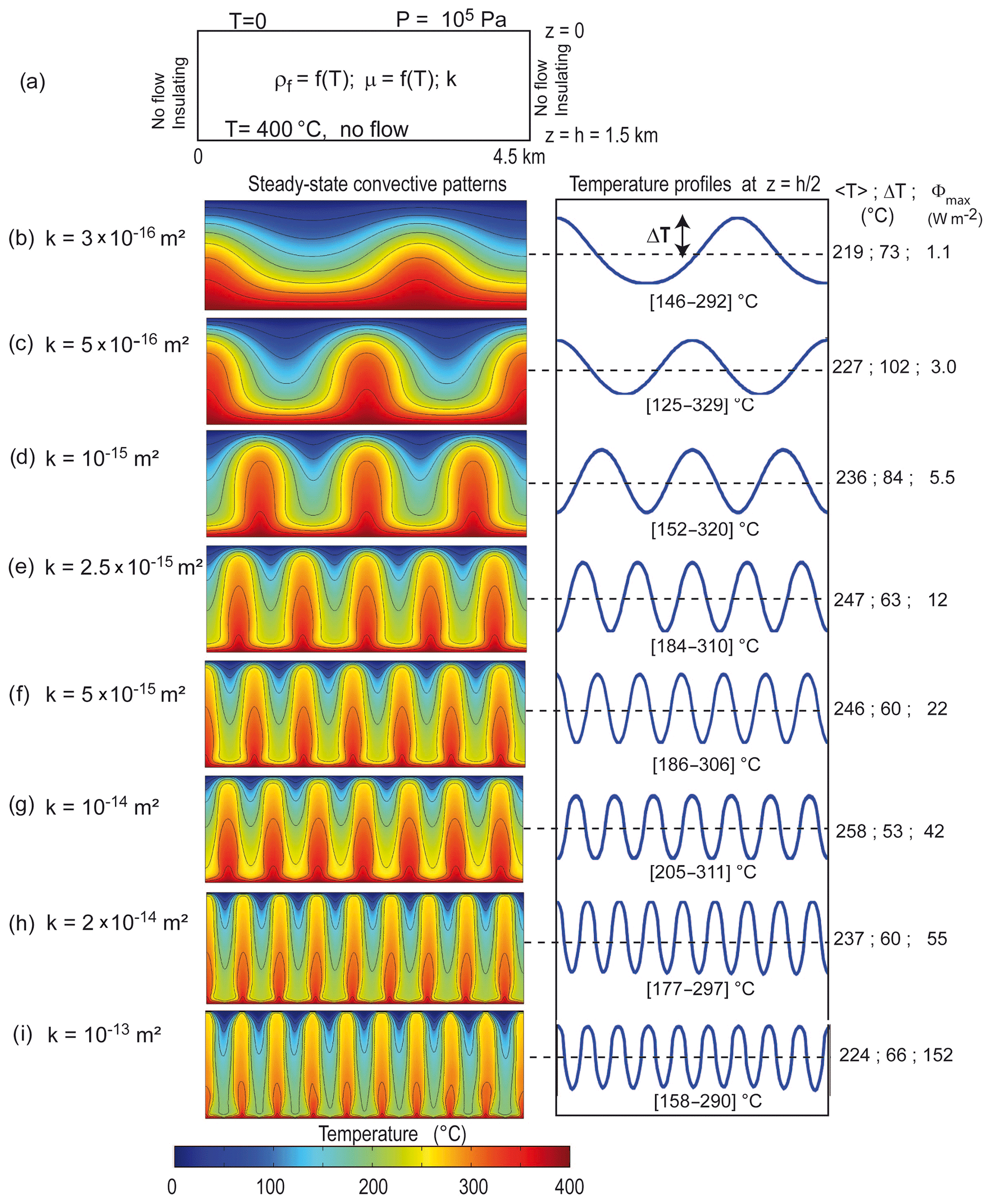
Figure 1 Steady-state temperature fields obtained for different values of the medium permeability. The left column shows temperature fields, and the right column illustrates a horizontal temperature profile at mid-depth. Averaged temperature at mid-depth (〈T〉), temperature anomalies (ΔT), and maximum heat flux carried by thermal plumes at the top surface are indicated on the right of each profile. The numerical setup and boundary conditions are illustrated in (a) and detailed in the text. For all experiments, the maximum mesh element size is 20 m. Hydrothermal convection (b) is observed for permeability around $\mathrm{3}\times {\mathrm{10}}^{-\mathrm{16}}$ m (a pure conductive regime is obtained for smaller permeability). The number of upwellings increases with increasing permeability. Above 10⁻¹³ m² , convection exhibits unsteady patterns, including typical Y-shaped and splitting plumes.

The second series of numerical experiments deal with 3D models of hydrothermal convection in a fault zone embedded in low-permeability host rocks. Benchmark tests are performed in order to reproduce the published results by Magri et al. (2017). For these particular 3D benchmark tests (detailed in Appendix B), a simplified density law (linear decrease with temperature) was imposed by the Magri et al. (2017) study. In the other 3D simulations (Figs. 8 to 14), a more realistic pressure and temperature dependence for fluid density is used, and a more realistic thermal boundary condition is applied at the bottom boundary (a fixed heat flow condition). One of the objectives of these 3D models is to understand how and where thermal anomalies develop. The role of the dip angle of the fault zone is tested, as is the role of permeability distribution.

3 Results from 2D models

3.1 Constant permeability

Figure 1 illustrates hydrothermal convection for constant permeability values from the onset of thermal convection (Fig. 1b) to vigorous convection, just before unsteady or turbulent convective patterns dominate. As already shown by many studies (e.g., Rabinowicz et al., 1998) the vigor of thermal convection (the number of upwellings or the maximum fluid velocity value) increases with permeability. Convective wavelength decreases with permeability, and up to eight internal upwellings (i.e., without considering the half plumes at lateral boundaries) are obtained in the most permeable case (10⁻¹³ m², Fig. 1i). While changes in the convective patterns are understandable (the more permeable the medium, the more active the convective regime), the evolution of thermal characteristics is less obvious. The right column in Fig. 1 shows horizontal temperature profiles at mid-depth, with numerical values of the horizontally averaged temperature 〈T〉, the temperature excess ΔT compared to this average and the maximum heat flux (Φ_max) carried by thermal plumes at the top surface. These latter values are in accordance with the results of Rabinowicz et al. (1998), as well as the spatial variation of the surface heat flux (see also Garibaldi et al., 2010). Due to asymmetric flow conditions at horizontal boundaries and nonlinear fluid properties, the averaged temperature at mid-depth exceeds 200 ^∘C, the temperature that would be present in the purely conductive case. When thermal convection occurs, this horizontally averaged value of 200 ^∘C can be obtained at mid-depth if fluid density varies linearly with temperature and when a no-flow condition – as at the bottom boundary – is imposed on the top surface.

Finally, Fig. 1 shows that while permeability increases, the increase in the horizontally averaged value 〈T〉 is not regular, nor is the temperature excess ΔT. Similarly, the minimum and maximum temperatures reached at mid-depths (values in brackets below horizontal temperature profiles) do not evolve regularly. The obtained convective patterns in Fig. 1 will be called finger-like upwellings as in, e.g., Zhao et al. (2003), with almost vertical isotherms bounding upwellings and downwellings, as also illustrated by Rabinowicz et al. (1998).

3.2 Depth-dependent permeability

In the shallow crust (above the brittle–ductile transition), permeability is expected to decrease with increasing lithostatic pressure (e.g., Manning and Ingebritsen, 1999; Saar and Manga, 2004; Achtziger-Zupančič et al., 2017), but this depth dependence may be less effective in highly permeable fault zones, like extensional faults in the Larderello and other geothermal systems (Della Vedova et al., 2008; Scibek, 2020). In the case of a constant-pressure boundary condition at the top surface (a more realistic condition for geological systems than a “no-flow” condition), the fact that permeability decreases with depth has important consequences for convective patterns. In Fig. 1, the finger-like upwellings are embedded within their cold counterparts (finger-like downwellings), thus exhibiting perfect geometrical symmetry. In contrast, when permeability decreases with depth, the number of upwellings decreases (Fig. 2). Case A corresponds to Fig. 1f, and cases B, C, and D illustrate experiments with an exponentially decreasing permeability with depth. The decrease in the number of upwellings can be explained by the asymmetric distribution of temperature and permeability: cold fluids are located in the most permeable zones, whereas hot fluids at depth encounter a less-permeable medium. Consequently, cold downwellings are favored and a general cooling is obtained in the last case (see mid-depth temperature profiles in Fig. 2). Contrary to the constant permeability cases, individual upwellings do not show a regular distribution of finger-like upwellings, since the cooling effect in the upper levels dominates and tends to destroy upwelling heads. According to their geometry, these upwellings will be named “triangular-like” upwellings (see in particular cases C and D).

3.3 Time-dependent permeability

3.3.1 From a depth-dependent to a constant permeability: instantaneous increase

Seismic activity could reactivate former deformation zones and thus instantaneously trigger a permeability increase (e.g., Sibson, 1992; Cox, 2010). Figure 3 illustrates the modifications of temperature patterns when a sudden increase in permeability is applied to case C in Fig. 2. The depth dependence of permeability is instantaneously canceled and a constant permeability of $\mathrm{5}\times {\mathrm{10}}^{-\mathrm{15}}$ m² is applied. Because permeability is increased at the bottom of the system, deep hot fluids can move upward more easily, and the triangular-like upwellings evolve toward a bulb-like geometry, with a shrinking tail and a large head. Surprisingly, the convective pattern illustrated in Fig. 1f (permeability of $\mathrm{5}\times {\mathrm{10}}^{-\mathrm{15}}$ m²) – i.e., with finger-like upwellings – is not recovered, although permeability is the same. This could be explained by the different initial thermal regimes, as detailed in Sect. 4.4.

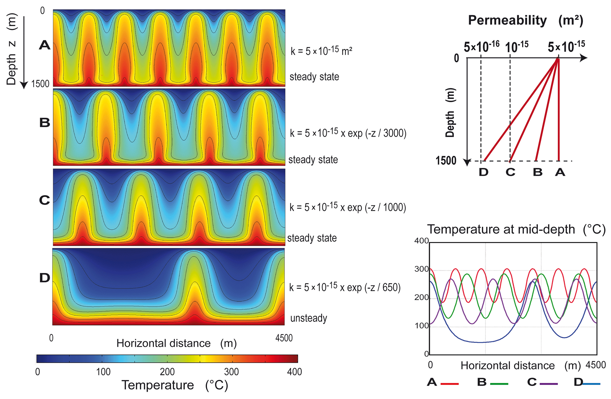
Figure 2 The effect of the depth dependence (decrease) of the permeability, here taken as exponential. The number of upwellings decreases when the depth dependence is accounted for: six internal upwellings are obtained for the constant permeability case (labeled A, top pattern) but only one for the steepest exponential decrease (D, bottom). Horizontal temperature profiles at mid-depth (bottom right) illustrate a major cooling effect, as well as the increasing temperature contrast between upwellings and downwellings when depth dependence is increased. See the text for explanations.

Figure 3 shows that the instantaneous increase in permeability has a warming effect at a depth of 600 m and a cooling effect at a depth of 1300 m. The warming effect corresponds to the larger head and the cooling effect to the shrinking tail. When compared to the preexisting case of triangular-like upwellings, temperature differences reach +50 and −70 ^∘C, respectively (Fig. 3d, e). Heat flux at the top surface increases regularly from 8 to 17 W m⁻² during 6000 years before reaching steady state.

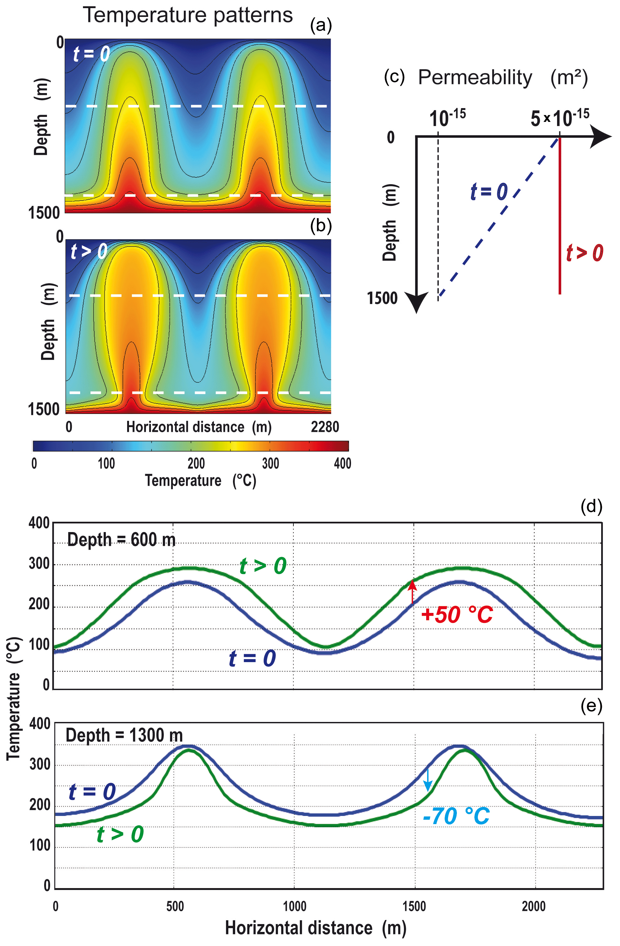
Figure 3 Effect of a sudden increase in permeability: from a depth-dependent variation (dashed line in c) to a higher constant permeability (red line). Temperature patterns (a, b) show that the initial triangular-like geometry (t=0) of the upwellings evolves toward a bulb-like geometry. Panels (d) and (e) show the temperature variations along the white dashed lines illustrated in the temperature patterns. The bulb-like regime involves higher positive temperature anomalies in the upper part of the system (up to 50 ^∘C) and higher negative temperature anomalies in the lower part (down to −70 ^∘C).

3.3.2 From a constant to a higher permeability: time-dependent increase

A progressive increase in permeability could be related to fluid–rock interactions that trigger the dissolution of minerals like quartz and calcite. This dissolution induces porosity generation, which in turn increases permeability (Scott and Driesner, 2018; Launay et al., 2019). One could also invoke tectonic processes like regional uplift, which modifies pressure conditions that partly control permeability. In contrast, progressive mineral deposition in the permeable structure can result in a permeability decrease (e.g., Lowell et al., 1993). Figure 4 illustrates the effects of a non-instantaneous increase in permeability for an initial convective pattern corresponding to a finger-like geometry (constant permeability of 10⁻¹⁵ m², case in Fig. 1d). Here, a permeability increase by a factor 20 is imposed over a total duration lasting 20 kyr (see Fig. 4a). This arbitrarily chosen duration allows for the identification of a transient unexpected warming event, highlighted by an increase in surface heat flux over the plume head from 5 to 35 W m⁻² during 200 years, reaching steady state at 33 mW m⁻² in the first 10 kyr. These timescales are similar to seismically induced fault permeability changes described by Howald et al. (2015).

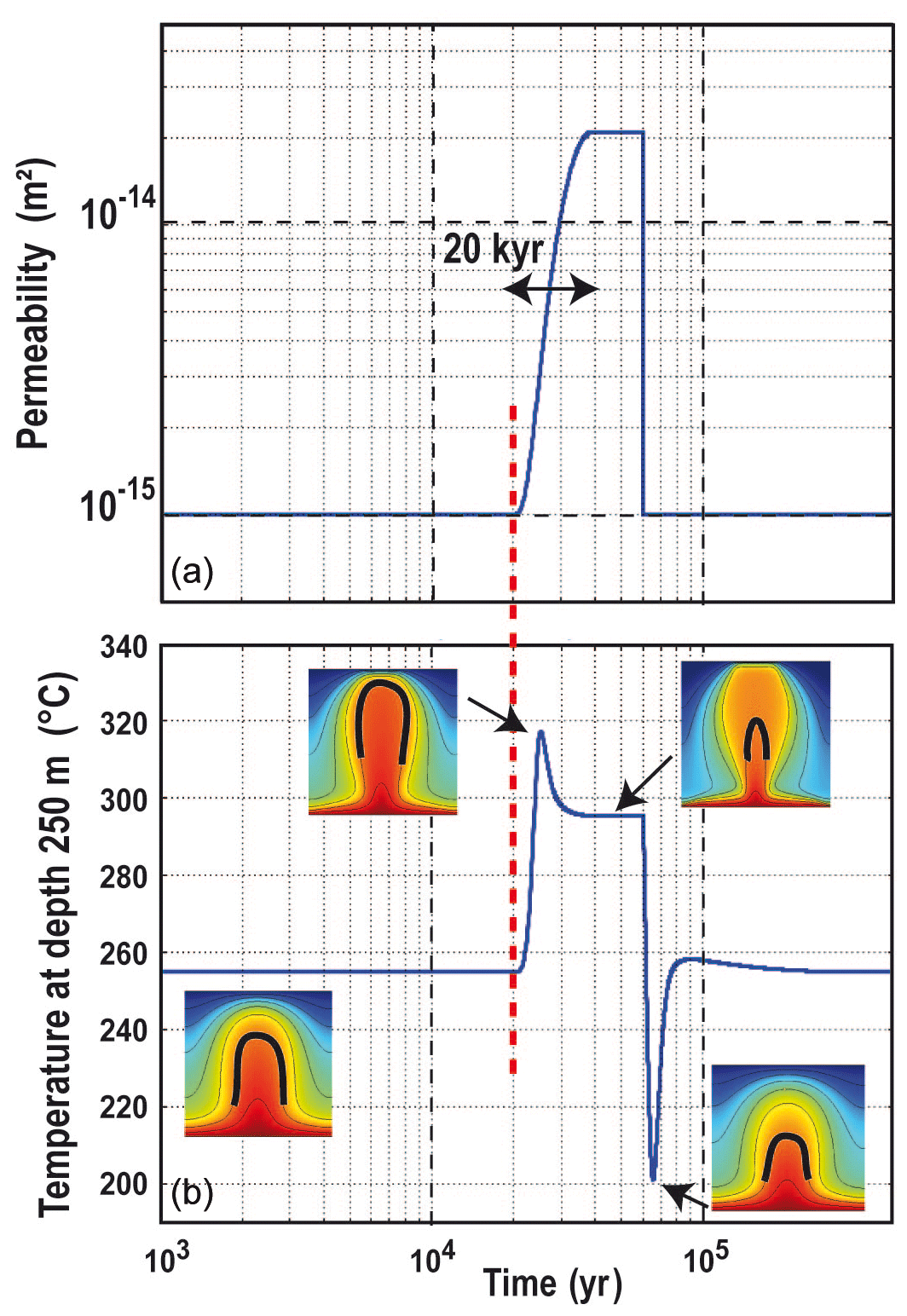
Figure 4 Effect of a time-dependent permeability increasing by a factor of 20 in 20 kyr. The finger-like geometry (lower left pattern) evolves towards a bulb-like geometry (upper right pattern). The temperature profile (b) shows short-duration heating and cooling events. The thick black contour on convective patterns corresponds to the 300 ^∘C isotherm. The color bar (not shown) is the same as in previous figures.

When permeability increases, hot fluid moves upward more easily, thus creating a warming effect at shallow depth from $t=\mathrm{2.0}\times {\mathrm{10}}^{\mathrm{4}}$ years to 2.5×10⁴ years (see temperature evolution at a depth of 250 m in Fig. 4b). As illustrated by colored patterns in Fig. 4, this first phase corresponds to the transition from a finger-like to a bulb-like pattern. After 2.5×10⁴ years, while permeability is still increasing, a cooling effect dominates, as illustrated by a temperature plot and colored patterns; the thick black line indicates the 300 ^∘C isotherm. When permeability is stabilized at $\mathrm{2}\times {\mathrm{10}}^{-\mathrm{14}}$ m², temperature becomes stable and the bulb-like pattern does not evolve. At time $t=\mathrm{6}\times {\mathrm{10}}^{\mathrm{4}}$ years, an instantaneous decrease in the permeability toward the initial value of 10⁻¹⁵ m² shifts the bulb-like geometry to the expected finger-like geometry. However, a short-duration important cooling stage (from 295 to 200 ^∘C) occurs during the instantaneous permeability decrease before the initial finger-like pattern is recovered.

3.3.3 Role of initial thermal regime: thermal inheritance

As illustrated by Figs. 1f and 3, different steady-state convective patterns can be obtained if the initial thermal regime differs: in the case of an initial purely conductive regime, a finger-like geometry is obtained with a permeability of $\mathrm{5}\times {\mathrm{10}}^{-\mathrm{15}}$ m² (Fig. 1f), while a bulb-like geometry is obtained when the initial thermal regime corresponds to triangular upwellings (Fig. 3). In the following, different initial thermal regimes are considered, and the evolving convective patterns are recorded when permeability is instantaneously increased up to a given value, which is identical for all cases. This type of simulation can illustrate what could happen in active and polyphased geological systems like orogenic belts.

In Fig. 5, initial permeability (hereafter noted k₀, patterns in the left column) is instantaneously increased to $\mathrm{5}\times {\mathrm{10}}^{-\mathrm{15}}$ m². The first experiment in Fig. 5 corresponds to Fig. 1f: starting from a conductive regime (flat isotherms), a finger-like geometry is obtained, with six internal upwellings. When the initial thermal regime corresponds to a convective pattern obtained with a permeability of $\mathrm{5}\times {\mathrm{10}}^{-\mathrm{16}}$ m², the finger-like upwellings evolve toward a bulb-like geometry (intermediate and final stages), and the number of internal upwellings slightly increases from one (initial and intermediate stages) to three (final steady state). In the last experiment in Fig. 5, the three initial upwellings are conserved, and here again, a bulb-like geometry is promoted. Conservation of the initial number of upwellings will be referred to in the following as thermal inheritance.

Figure 5 Illustration of thermal inheritance. For the three cases, the final permeability is the same but the initial thermal regime differs. In the first case (a), the initial thermal regime is purely conductive (top left). A finger-like morphology is obtained for the upwellings. In the two other cases (b, c), the convective pattern appears to be controlled or influenced by the initial one. A bulb-like morphology is promoted for the upwellings. The color bar (not shown) is the same as in previous figures.

Figure 6 shows similar experiments for different box lengths (5, 7, and 10 km): an instantaneous increase in the initial permeability k₀ is imposed. For each experiment from (a) to (h), the initial thermal regime is on the top and the final pattern is below. Figure 6a corresponds to the conditions in Fig. 1f, but the box length has been slightly increased (5 km instead of 4.5 km). It follows that seven internal finger-like upwellings are obtained (and not six as in Fig. 1f). For the same box length, the two other experiments (Fig. 6b and c) illustrate thermal inheritance: three internal upwellings are conserved in Figs. 6b and four upwellings in Fig. 6c. As in Fig. 3, the instantaneous permeability increase results in shrinking of the upwelling tail (see white arrows), thus promoting bulb-like geometries. Without detailing the other experiments for box lengths of 7 and 10 km (Fig. 6d to h), it can easily be seen that thermal inheritance is the rule. For each case, the final convective pattern appears to be controlled by the initial one (same number of upwellings).

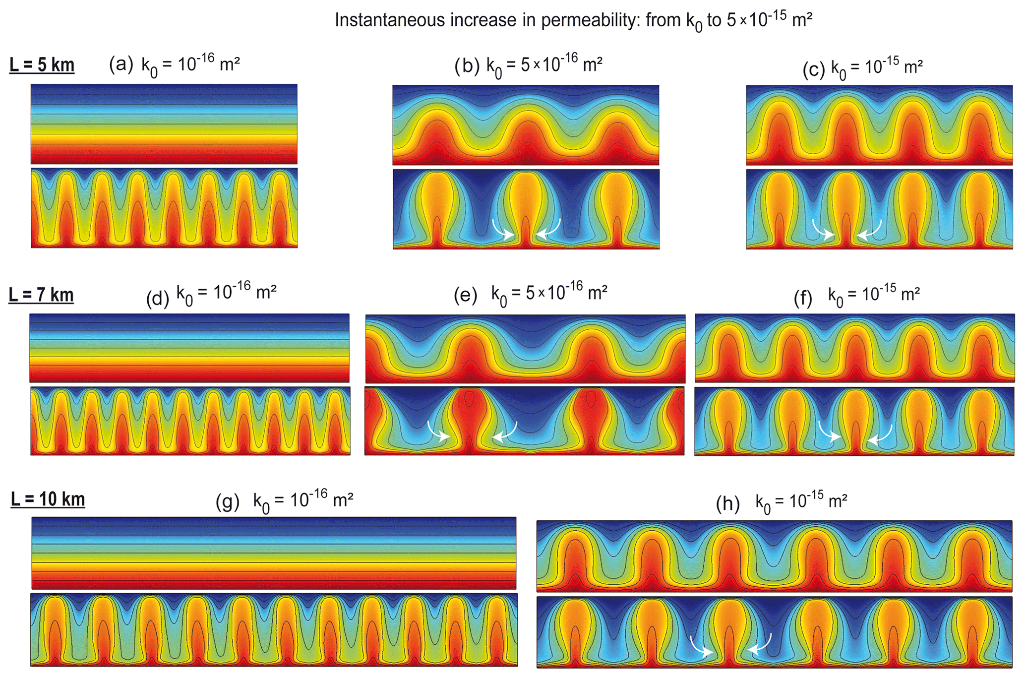
Figure 6 Additional experiments illustrating thermal inheritance for three distinct box lengths L. Initial (t=t₀) thermal regimes correspond to the figures on the top, obtained with the permeability k₀. At t>t₀, for the eight experiments, permeability is instantaneously increased from k₀ to $\mathrm{5}\times {\mathrm{10}}^{-\mathrm{15}}$ m² , and the obtained regime after a few hundred years is shown at the bottom of each experiment. For each box length, the initial thermal regime can represent a conductive regime (cases a, d, and g), a slightly convective regime (b, e), or a more vigorous convective regime (c, f, h). For each case, the obtained convective pattern is strongly controlled by the initial one; i.e., the location of upwellings is dictated by that of the previous ones. Note that the finger-like shape of upwellings (a, d, g) is changed to a bulb-like shape with a shrinking base (white arrows) when the initial thermal regime is not conductive. The color bar (not shown) is the same as in previous figures.

3.4 Case of high permeability: pulsating plumes

When permeability suddenly increases (Figs. 3 to 5), the bulb-like geometry is favored because hot buoyant fluid has less resistance to upward flow, and fluid velocity increases. In the case of a high permeability involving fluid velocity greater than $\sim {\mathrm{10}}^{-\mathrm{7}}$ m s⁻¹, the velocity increase separates the plume head from its tail, as already noted by Coumou et al. (2006) and Fontaine and Wilcock (2007), who observed “individual upflow zones”. Figure 7 illustrates such a case in which initial permeability (depth-dependent permeability with a maximum value of 10⁻¹⁴ m²) is increased to a constant value of $\mathrm{2}\times {\mathrm{10}}^{-\mathrm{14}}$ m² (Fig. 7a). The initial convective pattern (triangular-like geometry) evolves promptly toward a bulb-like geometry and a pulsating behavior is observed, exhibiting several individual stages of the hot upwelling. Even if this convective regime is close to a chaotic behavior, one can define a time period of 240–250 years in accordance with the results of Fontaine and Wilcock (2007). Indeed, Fig. 7 shows that similar patterns are observed at time t₀+50 years and t₀+300 years or at time t₀+160 years and t₀+400 years.

Figure 7 Instantaneous increase in the medium permeability (from ${\mathrm{10}}^{-\mathrm{14}}\exp (-z/\mathrm{650})$ at t=t₀, to $\mathrm{2}\times {\mathrm{10}}^{-\mathrm{14}}$ m² , at t>t₀) resulting in a high-velocity upwelling, wherein the central blob does not lose much energy during ascent. (a) Steady-state triangular-like upwelling at t=t₀ and permeability function; (b) temporal evolution of the convective pattern showing the detachment of a high-temperature “blob” (T>300 ^∘C); (c) plots of vertical temperature profiles taken at the blob vertical axis (red vertical line in the top left pattern) for each time step shown in (b). The color bar (not shown) is the same as in previous figures.

Starting from the initial stage, deep hot fluid accelerates and finally forms an isolated blob of fast hot fluid separated from the tail. The black-contoured area in Fig. 7b contains fluid hotter than 300 ^∘C. Before the separation occurs, maximum fluid velocity reaches $\mathrm{3}\times {\mathrm{10}}^{-\mathrm{7}}$ m s⁻¹ (9 m yr⁻¹), whereas typical fluid velocity is around $\mathrm{5}\times {\mathrm{10}}^{-\mathrm{8}}$ m s⁻¹ for a permeability of $\mathrm{5}\times {\mathrm{10}}^{-\mathrm{15}}$ m² and around 10⁻⁸ m s⁻¹ for a permeability of 10⁻¹⁵ m². Figure 7c illustrates the thermal signature of this ascending blob (or pulsating plume). It can be seen that vertical temperature profiles have a locally negative temperature gradient at t₀+120 years and after. The multiple blobs illustrated at t₀ + 450–475 years are also visible on labeled temperature profiles.

4 Results from 3D models

In the following, a simplified 3D numerical approach is focused on the case of a finite-sized fault zone embedded in a less-permeable host rock. In order to validate our numerical approach and procedure, we first performed benchmark tests on the basis of a recently published study, wherein different teams worked on the same numerical scenario but with different finite-element numerical codes (Magri et al., 2017). As emphasized by Magri et al. (2017), despite similar convective patterns, some quantitative differences in the results were observed and interpreted to be due to “discretization errors” (spatial and temporal) or different “solver settings”. Consequently, our benchmark test is also expected to qualitatively reproduce the same convective patterns.

Benchmark tests and results are described in Appendix B. These tests consider a thin (40 m wide) fault zone with simplified fluid properties identical to those of the Magri et al. (2017) study. In Appendix B, convective patterns, thermal and velocity fields, and temperature anomalies are detailed. The following experiments (below) are focused on the case of thicker permeable fault zones (100–400 m), for which the fluid density law is more realistic than in the benchmark tests since it is temperature- and pressure-dependent (see Appendix A). The thermal boundary condition at the bottom of the box (depth 5500 m) is not 170 ^∘C as in Magri et al. (2017) and in our benchmark experiment, but it corresponds to a more realistic fixed heat flow condition of 100 mW m⁻², a typical value in favorable areas for geothermal exploration (e.g., Blackwell et al., 2006; Cloetingh et al., 2010; Erkan, 2015). However, for the problem geometries considered, this high basal heat flow will not induce temperature values higher than 210 ^∘C. To involve temperatures around 300–350 ^∘C, one would need to impose a basal heat flow condition around 180 mW m⁻², a value considered to be too extreme for the purpose of this study (see, however, Della Vedova et al., 2008, wherein basal heat flow in Tuscany, Italy, would be around 150–200 mW m⁻²). In the following, the role of a depth-dependent permeability and the effect of the fault dip angle are investigated. To avoid edge effects, the case of a longer fault is also presented.

4.1 Case of a vertical fault zone with a constant permeability

In the following experiment, which is derived from the benchmark case, the fault zone is 400 m wide and 5 km deep, does not outcrop at the surface, and does not reach the bottom of the box (depth 5.5 km). Its dip angle will be varied as will its permeability. An averaged heat production of 2 µW m⁻³ is imposed in the entire model to account for representative radiogenic heat production in a shallow granitic crust (Jaupart and Mareschal, 2011; Artemieva et al., 2017). The top left of Fig. 8 shows some of the boundary conditions, the others being no flow and no thermal exchanges.

In Fig. 8, the fault permeability (k_F) is fixed at 10⁻¹⁴ m², while the host rock is supposed impervious ($k_{\mathrm{H}}={\mathrm{10}}^{-\mathrm{18}}$ m²). The initial thermal regime for all the following 3D models corresponds to a purely conductive regime. Figure 8 illustrates the time evolution of positive temperature anomalies (colored zones in the middle plane of the fault zone, defined as temperature excess when compared to the conductive case) together with the domain in which temperature is greater than 130 ^∘C (grey areas). The time evolution of temperature at a depth of 2.5 km within the fault zone is also shown.

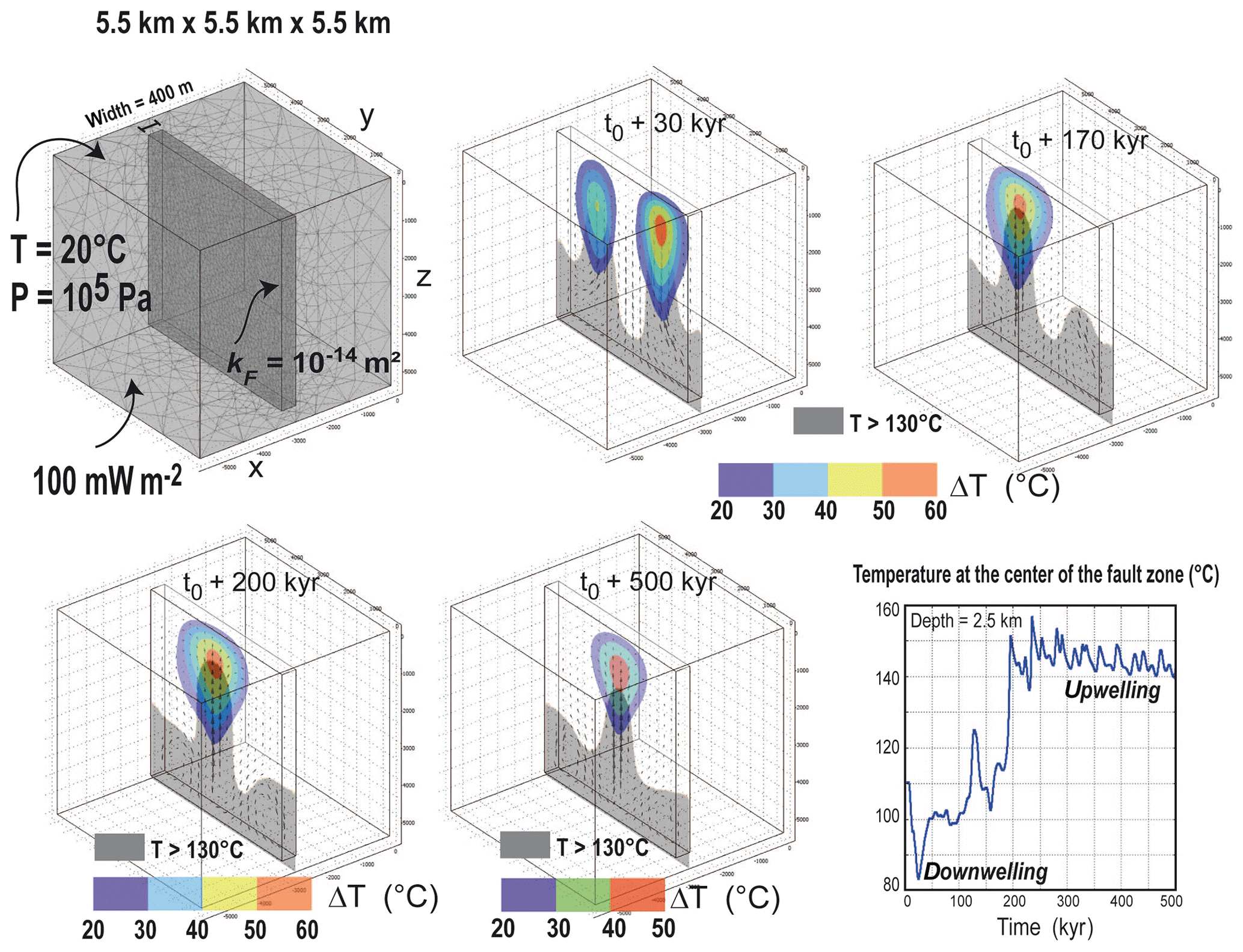
Figure 8 Case of a wide vertical fault zone in a 3D block, with realistic fluid properties and boundary conditions. Fault permeability is fixed at 10⁻¹⁴ m². Positive temperature anomalies greater than 20 ^∘C are colored in the middle plane of the fault zone. Zones in which temperature exceeds 130 ^∘C are shown in grey. Temperature evolution at the center of the fault zone illustrates the transition from a downwelling to an upwelling from 150 to 200 kyr.

Temperature anomalies in 3D exhibit a hot air balloon morphology (see one perpendicular view in Fig. 9), whereby the maximum value exceeds 50 ^∘C for at least 200 kyr. This same shape was visible in the benchmark experiment (Appendix B, Fig. B1). This morphology could be called the “geothermal reservoir”, whose size would be described by a given critical value of the temperature anomaly (e.g., ΔT>30 ^∘C). The absolute temperature value at a depth of 2.5 km also exceeds 150 ^∘C between 200 and 340 kyr (see temperature evolution in the lower right of Fig. 8). During the first 200 kyr, the convective pattern is mainly dominated by a central cold downwelling and two adjacent upwellings. With time, the pattern reverses for a single hot central upwelling. This flow reversal was also observed for an inclined fault zone (see below).

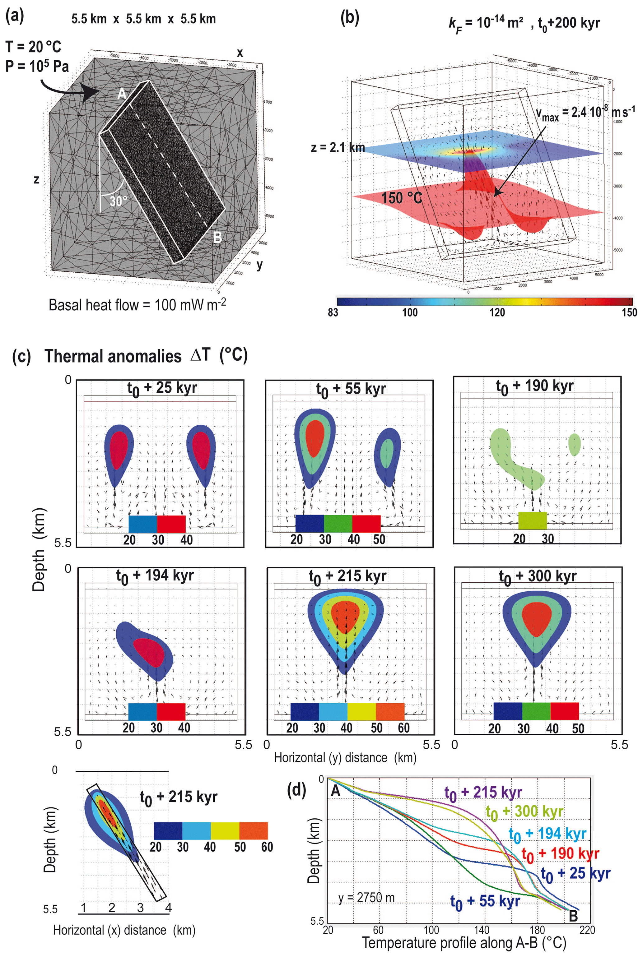
Figure 9 (a) Similar experiment as in Fig. 8 but for an inclined (30^∘) fault zone. (b) A temperature of 150 ^∘C is reached at a depth of 2.1 km. The color bar corresponds to temperature values at a depth of 2.1 km; (c) temporal evolution of thermal anomalies (colored zones) viewed in a vertical plane: a similar transition from two upwellings to a single central one is observed. The perpendicular view at bottom left illustrates the lateral diffusion of the anomaly within the host rock. (d) Temperature evolution within the fault zone along the A–B profile.

4.2 Similar case for an inclined fault

Figure 9 shows an experiment in which all parameters are identical to the previous one, except for the fault dip angle, here chosen at 30^∘ from the vertical. Figure 9b illustrates the temperature field at t₀+200 kyr at a depth of 2.1 km (colored plane), where a temperature of 150 ^∘C is attained; it also shows the distorted 150 ^∘C isotherm (in red), reflecting the upward fluid circulation rising at a maximum velocity of $\mathrm{2.4}\times {\mathrm{10}}^{-\mathrm{8}}$ m s⁻¹ (0.75 m yr⁻¹). Figure 9c illustrates the time evolution of temperature anomalies from two “balloons” to a single one at times greater than t₀+190 kyr. During the transition from two to one single upwelling, the temperature anomaly decreases in amplitude and then recovers to values greater than 50 ^∘C (see time t₀+215 kyr). At the bottom left of Fig. 9c, a lateral view of the same temperature anomaly shows that (i) the temperature anomaly extends laterally to more than 500 m away from the fault zone boundaries, and (ii) the maximum range of 50–60 ^∘C extends from a depth range of ∼1.0 to 2.2 km. Figure 9d shows a downward temperature profile along the fault (A–B in Fig. 9a). The upward temperature anomaly is clearly visible and appears to be maximum at time t₀+215 kyr.

4.3 Cases with a depth-dependent permeability

In the four experiments in Fig. 10, a depth-dependent permeability (exponential decrease) is imposed within the fault, and the dip angle varies from 0 (vertical) to 45^∘. The maximum fault permeability here is 20 times higher than in Figs. 8 and 9. For each dip angle, the transient evolution of positive thermal anomalies is illustrated.

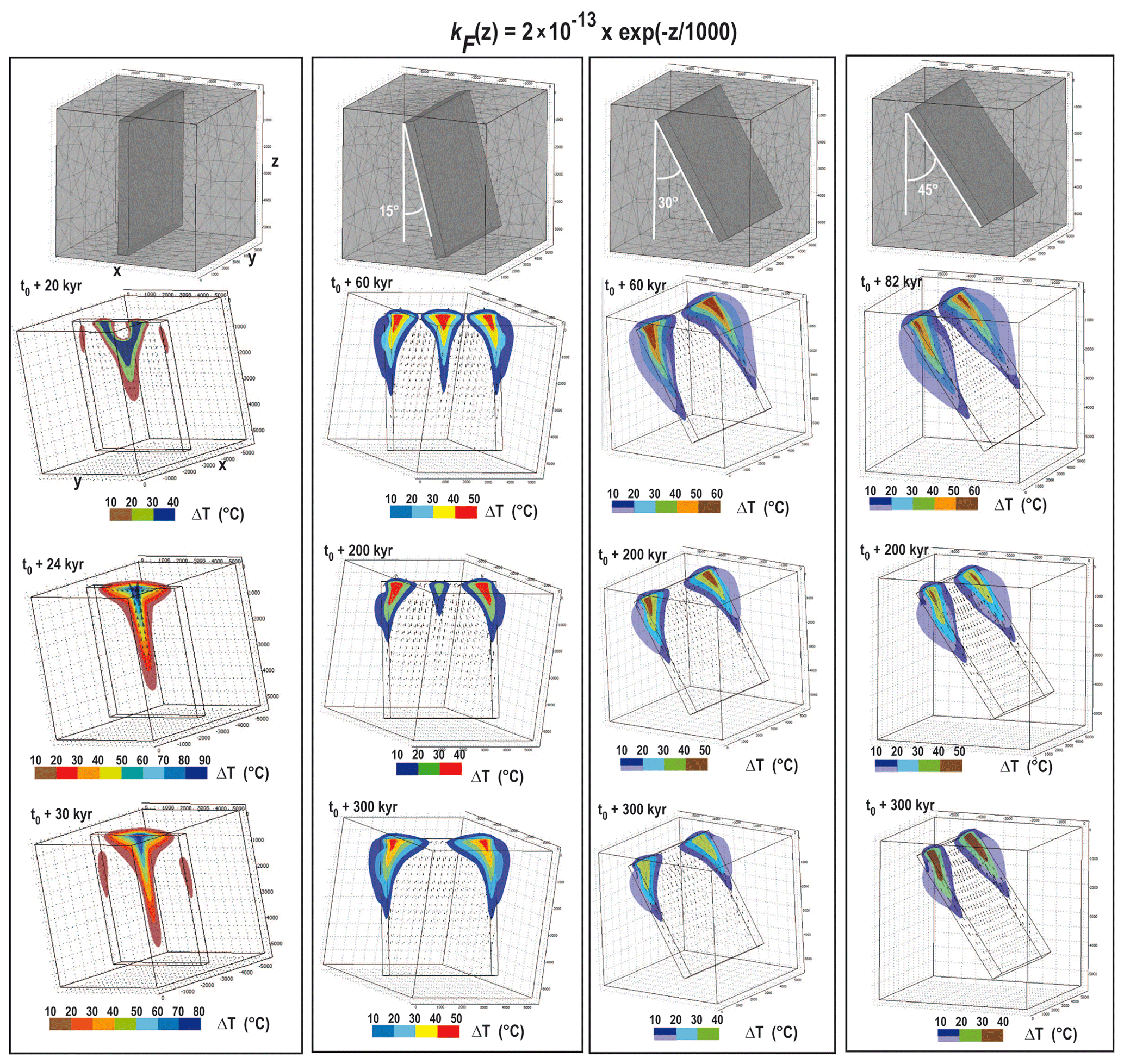
Figure 10 Four experiments with realistic fluid properties and a depth-dependent permeability with a dip angle of 0, 15, 30, and 45^∘. Few differences exist between the two higher dip angles. The largest temperature anomaly amplitudes are obtained in the vertical case (left) and during the first tens of thousands of years. In the second case (15^∘ dip angle), a transient anomaly disappears after 200 kyr.

In the case of a vertical fault zone (left column), a quasi-steady-state convective pattern is reached at time t₀+24 kyr. The initial anomaly exhibits a “Y-shaped” pattern (t₀+20 kyr) with a temperature anomaly lower than 40 ^∘C. With time, the Y-shaped anomaly evolves towards a “funnel-shaped” pattern (t₀+30 kyr) with a much larger temperature anomaly. Because permeability is higher at shallow depths, the anomaly expands laterally near the surface. From the top of the fault zone (at a depth of 500 m) to a depth of ∼1.0 km, a temperature anomaly greater than 80 ^∘C (dark blue zone) and around 500 m wide establishes.

For the three cases with inclined fault zones (dip angles of 15, 30, and 45^∘), time evolution is much longer since quasi-steady-state convective patterns are reached only after 200 kyr. There are two main differences between these three experiments and the previous one (i.e., the vertical case). The first is that the number of anomalously warm upwellings increases. At time t₀+60 kyr and for a dip angle of 15^∘, three anomalies (greater than 40 ^∘C) are identified. With time, the central one disappears because a central downwelling establishes, leaving two positive anomalies at fault edges. The second major difference is the value of the temperature anomalies, which do not exceed 50–60 ^∘C in the case of an inclined fault zone. These results are consistent with the 2D models of Duwiquet et al. (2019), who also found higher thermal anomalies for vertical fault zones.

4.4 Case of a longer fault

The curved shape of the lateral anomalies in Fig. 10 (for inclined fault zones) might be due to side-boundary effects since the fault length is the same as the fault height. The following experiments illustrate the case of a longer (15 km) fault zone with a maximum permeability of $\mathrm{5}\times {\mathrm{10}}^{-\mathrm{13}}$ m². In Fig. 11, the fault width is reduced to 100 m and the fault dip angle is varied. In Fig. 12, the fault dip angle is fixed at 30^∘, while the fault width is varied from 100 to 400 m. Snapshots of experiments correspond to time steps during which the thermal anomaly is maximum (see temporal evolution in Fig. 11a and horizontal temperature profiles in Fig. 11b).

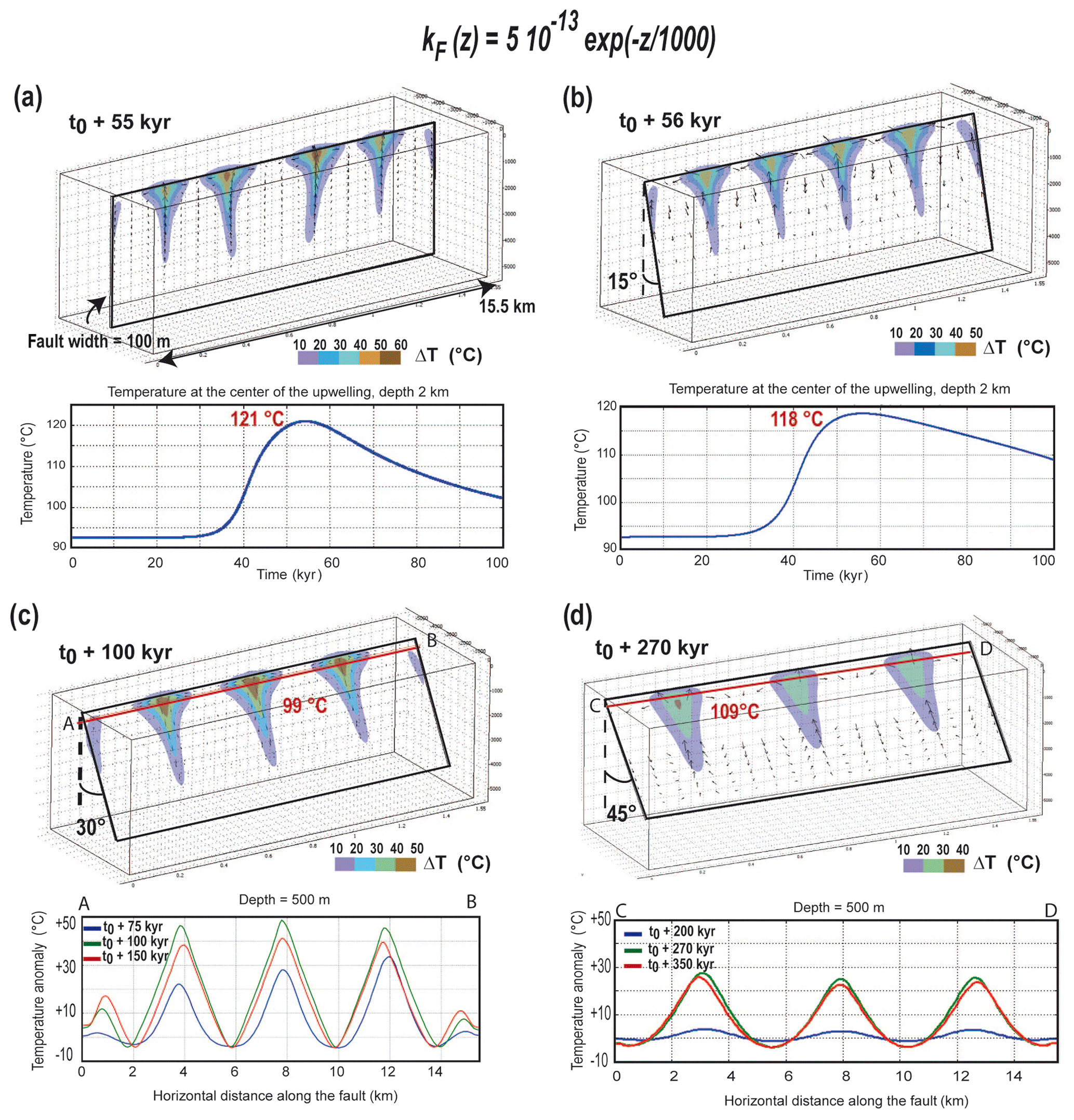
Figure 11 Experiments with a longer (15.5 km long) fault with different dip angles (0, 15, 30, and 45^∘). Permeability is depth-dependent with a maximum value of $\mathrm{5}\times {\mathrm{10}}^{-\mathrm{13}}$ m² for each case. The obtained temperature anomalies slightly exceed 50 ^∘C in the vertical case only. Cross sections illustrate the maximum temperature anomaly obtained during the entire experiment. The time evolution of temperature (top) or temperature anomalies (bottom) is shown beneath the temperature anomaly patterns.

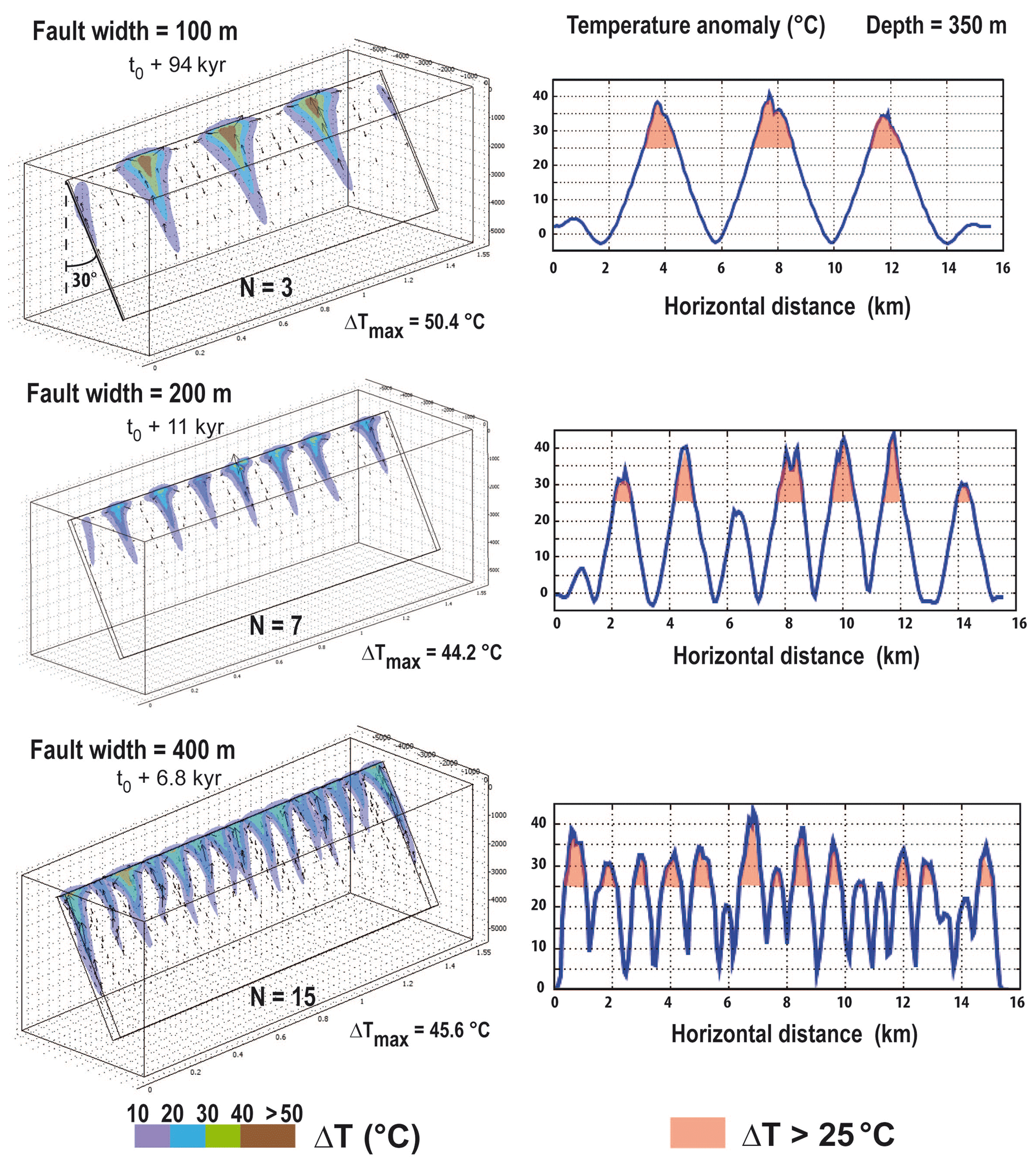
Figure 12 Effect of fault width on temperature anomaly pattern for a dip angle of 30^∘ and the same permeability law as in Fig. 11. Values of maximal temperature anomalies are similar, but the wider the fault, the more numerous the positive thermal anomalies. Temperature anomalies greater than 25 ^∘C at a depth of 350 m are highlighted on the right.

In all experiments, funnel-shaped thermal anomalies develop, controlled by the exponential decrease in fault zone permeability. Except for the vertical case (Fig. 11a), thermal anomalies do not exceed 50 ^∘C. The maximum temperature anomaly is reached more rapidly when the fault dip angle is small (at t₀+55 kyr and t₀+56 kyr for 0 and 15^∘, respectively) or when the fault width is large (at t₀+6.8 kyr for a 400 m wide fault). The two plots of temporal evolution in Fig. 11a show that the maximum temperature anomaly remains elevated (above 25 ^∘C) during ∼20 kyr, a duration which could be regarded as representative of the lifetime of a geothermal system. Obviously, this value is associated with the permeability distribution.

Figure 12 shows that the wider the fault, the higher the number of funnel-shaped anomalies. This results in an almost continuous thermal anomaly at shallow depth (see horizontal profiles at a depth of 350 m, right column in Fig. 12). Figure 13 illustrates thermal diffusion in host rocks: the anomalously high temperatures extend over a distance of 2.4 km (1200 m for each side). Figure 13 also illustrates that a vertical fault zone (left case) induces a much higher-temperature anomaly (64 ^∘C at a depth of 500 m) than an inclined fault zone (only 38 ^∘C), as observed in Figs. 10 and 11.

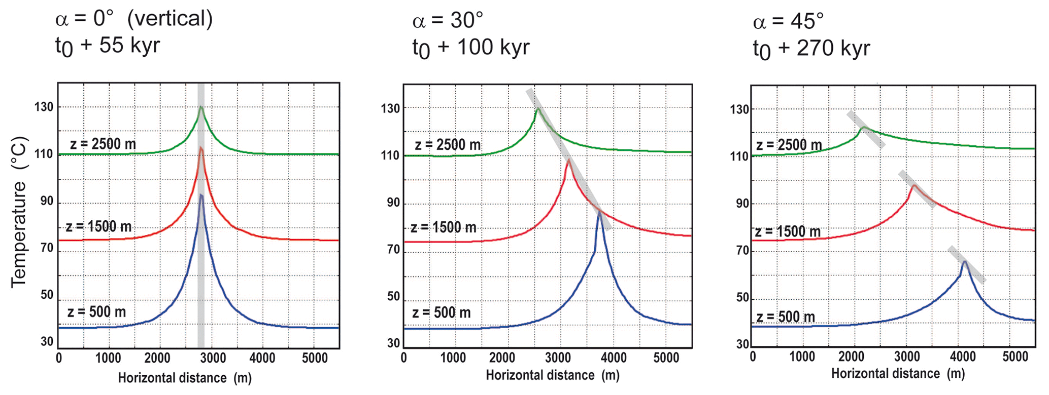
Figure 13 Effect of fault dip angle (angle is illustrated by grey rectangles) on horizontal profiles of temperature, perpendicular to the fault zone, at the time when the temperature anomaly is maximum (indicated on top of each case). While the lateral diffusion length remains similar (∼1200 m on each side at a depth of 500 m and ∼ 800–900 m at a depth of 2500 m), the amplitude is clearly greater in the vertical case (∼ 55 ^∘C at a depth of 500 m in the vertical case and ∼ 28 ^∘C for a dip angle of 45^∘).

To this point, all of our numerical experiments have assumed the host rock to be impermeable. Here we consider some of the effects of permeable host rock. Figure 14 shows the temporal evolution of thermal anomalies superimposed on the temperature field within a 100 m wide vertical fault zone. Two different permeability fields in the fault zone are illustrated, and the ratio between fault permeability and host rock permeability equals 20 and 50. While one internal upwelling dominates in the low-ratio case, four upwellings are obtained in the case of the more permeable fault zone. Because fluid velocity is smaller in the low-ratio case (the maximum temperature anomaly is reached at t₀+200 kyr versus t₀+45 kyr in the permeable case), thermal diffusion and heat advection into the host rocks are more effective (compare the two horizontal map views at the bottom of Fig. 14). Although the along-fault dimensions of the two thermal anomalies are similar (2.3 and 2.5 km), their width differs by almost a factor of 2. The maximum temperature anomaly reaches 78 ^∘C in the low-ratio case and 66 ^∘C in the permeable case. From these two experiments, one could conclude that the volume and the potential of the geothermal reservoir are greater for the smaller permeability ratio, but additional experiments with higher permeability ratios, as in Duwiquet et al. (2019), are required. One last experiment, not shown here, with an imposed basal heat flow was 150 mW m⁻² was carried out with a permeability ratio of 100. Three funnel-shaped anomalies developed, with a maximum amplitude of 120 ^∘C centered at 500 m of depth. For this particular experiment, temperatures of 150 ^∘C were reached at a depth of 750 m. Temperature anomalies exceeded 70 ^∘C over a depth range of 3 km and a lateral dimension of 700 m.

Figure 14 Effect of permeability ratio between a vertical fault zone and the host rocks: $k_{\mathrm{F}}/k_{\mathrm{H}}=\mathrm{20}$ (left) and 50 (right). The maximum temperature anomaly is reached at time t₀+200 kyr (left) and t₀+45 kyr (right). The bottom images show temperature anomalies from above at a depth of 500 m. While the maximum amplitudes of the anomalies do not differ much (66 and 78 ^∘C), the lateral diffusion lengths strongly differ (2.3 and 1.4 km wide).

5 Discussion

The main objective of this study was to investigate the various possible convective patterns and the associated thermal anomalies in a permeable fault zone. 2D experiments were first performed to validate our numerical approach by reproducing the published results of Rabinowicz et al. (1998) and can be viewed as fluid circulation models along a fault plane, without accounting for mass exchanges with the host rock. Some particular processes were highlighted (such as the thermal inheritance mechanism) and are further discussed below. When more realistic fault zones are considered, i.e., when damage zones of several tens to hundreds of meters are taken into account, 3D experiments are required, since convective patterns are expected to also depend on host rock properties. In the 2D experiments, boundary conditions and fluid properties were chosen to reproduce the results by Rabinowicz et al. (1998), and the fluid density law in particular was simplified (Appendix A). In the 3D experiments, more realistic physical conditions are applied: fluid density is temperature- and pressure-dependent, and the bottom thermal boundary condition corresponds to a fixed heat flow of 100 mW m⁻². Our approach differs from the “discrete fracture flow” approach whereby fracture networks consist of discrete thin fault planes (e.g., Mezon et al., 2018). Here, the fracture flow approach is not appropriate because the thickness of crustal fault zones may exceed hundreds of meters.

5.1 2D convective patterns

In the first series of 2D models, the well-known finger-like convective pattern was reproduced for a constant permeability (Fig. 1). Because of lithostatic pressure, permeability generally decreases with depth, and the use of a more realistic permeability distribution appears to change the finger-like pattern towards a triangular-like pattern (Fig. 2) with a dominant cooling effect. Indeed, the most permeable levels being at shallow depths, cold downwellings are favored. This may explain why, along permeable fault zones, hot upwellings (evidenced by the emergence of thermal springs) are not numerous and irregularly spaced.

Equivalent effects might be caused by the presence of significant topography (>1500 m), causing infiltrating cold fluids to dominate and prevent hot fluids from rising to the surface, except in a few locations (see the clusters of thermal springs in the Pyrenees in Taillefer et al., 2017). The role of topography in the location of thermal springs in the Jordan rift valley has also been investigated by Magri et al. (2015), who illustrated the coexistence of topography-driven and buoyancy-driven flow. Topography-driven flow can predominate and modify the convective patterns. Nevertheless, the results shown in Fig. 2 indicate that when topography is not important, depth-dependent permeability may have similar consequences.

In Figs. 3 and 4, instantaneous and continuous increases in permeability modify the initial convective pattern (triangular-like or finger-like) to form bulb-like convective patterns, with a significant temperature increase at shallow depth. Conversely, a decrease in permeability recovers the finger-like pattern, accompanied by short-duration cooling (Fig. 4). This process might be of major importance for geothermal exploration around active fault zones, for which permeability is probably at its maximum. In other words, active fault zones could host geothermal reservoirs with a kilometer-scale bulb-like geometry (see also Patterson et al., 2018a; Wanner et al., 2019).

The thermal inheritance concept illustrated in Figs. 5 and 6 may be relevant for a number of geological processes involving the circulation of deep hot fluids. Studies on gold metallogeny (orogenic gold deposits, gold deposits in banded iron formations, gold in volcanic massive sulfides) have often suggested polyphased mineralizing events (e.g., Bonnemaison and Marcoux, 1990; Coumou et al., 2009; Lawley et al., 2015; Gourcerol et al., 2020). This mechanism could indeed be at the origin of polyphased hydrothermal ore deposits in the sense that a structure already mineralized could be more favorable for focusing the latter hydrothermal stages. While structural inheritance has been invoked many times to explain the strain localization or tectonic history of mountain belts (e.g., Jammes et al., 2013), thermal inheritance appears to be another physical mechanism that may play an important role in the wide range of thermomechanical processes.

Finally, the pulsating behavior observed in Fig. 7 has been used by Deveaud et al. (2015) to suggest one possible dynamical mechanism at the origin of rare-element pegmatite emplacement. Indeed, these magmatic liquids have an extremely low viscosity (e.g., Bartels et al., 2013). Consequently, the associated dynamic permeability (the ratio between static permeability and fluid viscosity) is anomalously high, and escape and detachment from a deep crustal magma source through permeable shear zones are facilitated. Successive separations from a magma source could explain the differences in chemical enrichment within a single pegmatite field (Melleton et al., 2015). The pulsating behavior observed in Fig. 7 was also suggested by Link et al. (2019) to help explain the multiphase gold mineralizing events in fault zones of the Pyrenees, south of France.

5.2 3D hydrothermal convection and temperature anomalies

The understanding of 3D hydrothermal convection in fault zones has progressed in the last decades. Recently, a new Rayleigh number expression based on fault geometry and on physical fluid and rock properties has proved to be better adapted than the Rayleigh theory to define the onset of thermal convection (Malkovski and Magri, 2016). Numerical modeling of 3D hydrothermal convection has considered numerous geological examples from the fractured oceanic lithosphere to fault zones (e.g., Rabinowicz et al., 1998; Fontaine et al., 2001; Zhao et al., 2003; Bächler et al., 2003; Kuhn et al., 2006; Baietto et al., 2008; Harcouët-Menou et al., 2009; Coumou et al., 2009; McLellan et al., 2010; Person et al., 2012; Andersen et al., 2015; Magri et al., 2016; Malkovski and Magri, 2016; Magri et al., 2017; Taillefer et al., 2018; Patterson et al., 2018a, b; Bauer et al., 2019). For each case, some surprising dynamical features were discovered, such as the thermal interference between separated fractures (Patterson et al., 2018b) and helicoidal fluid flow pathways (Magri et al., 2016). However, the anomalously high temperatures at shallow depths were not necessarily studied in detail.

Patterson et al. (2018a) have reproduced typical convective patterns such as those described in our 3D benchmark tests (Fig. B1 in Appendix B), but for thinner fractures (up to 10 m wide) of elliptical geometry. The values of their obtained temperature anomalies (see their Fig. 3) are much smaller (not greater than ±15 ^∘C) than those obtained in our benchmark tests, wherein the fault width equals 40 m. However, the geometry of their thermal anomalies was similar and shows a hot air balloon morphology. Person et al. (2012) illustrated the role of fault intersections in temperature anomalies at the surface for fault permeability values ranging from 2 to $\mathrm{7}\times {\mathrm{10}}^{-\mathrm{13}}$ m². Transient evolution shows that temperature anomalies up to 92 ^∘C can be achieved. Yet, in their experiments, fault widths are small (10 and 20 m), and a “spring” thermal boundary condition (no vertical temperature gradient) was imposed at the surface in the lowlands of their model, spanning the vertical fault zones. This boundary condition may favor the upflow of deep hot fluids within these highly permeable structures, and their temperature anomalies might be overestimated. Our 3D models show that, without imposing a spring condition at the surface, a temperature anomaly up to 90 ^∘C may indeed occur at the top of a non-outcropping vertical fault zone (Fig. 10, vertical case).

According to previous studies wherein the width of the fault zone is smaller than 100 m, and also considering our results in which widths exceed 100 m, it seems that the wider the fault, the larger the temperature anomaly: around 30 ^∘C for a 40 m wide fault zone (Appendix B), around 50–60 ^∘C when the fault width equals or exceeds 100 m (e.g., Fig. 11), and up to 80–90 ^∘C when the fault zone is wide and vertical (Figs. 10 and 14). Nevertheless, this is not the case for the dipping fault in Fig. 12, for which only the fault zone width varies from 100 to 400 m, and the temperature anomaly remains around 50±10 ^∘C. The most important parameter could be the fault dip angle, as illustrated in Fig. 10 and as suggested by Achtziger-Zupančič et al. (2016). However, permeability distribution clearly plays a role, and it is probably the combination of fault width, fault permeability distribution, and dip angle that controls the movement of energy towards the surface (e.g., Roche et al., 2019). A more systematic study of all these parameters should allow for the construction of a regime diagram for 3D convective patterns.

5.3 Morphology of thermal anomalies

Wanner et al. (2019) modeled the effect of a vertical upflow in a permeable (10⁻¹³ m²) zone (area of 150 m × 100 m). They obtained an ellipsoidal vertical thermal plume providing 120 ^∘C at a depth of 2 km. The morphology of their thermal anomaly is close to our hot air balloon morphologies (Figs. 8 and 9), although boundary conditions differ: in their model, an overpressure is imposed at the base of the upflow zone, and a fixed temperature of 4 ^∘C is imposed on the top surface, preventing any lateral expansion of the anomaly (our funnel-shaped anomalies). The fact that we obtained a temperature of 150 ^∘C at a depth of 2.1 km (Fig. 9b, wherein fault zone permeability is 10⁻¹⁴ m²) may be due to buoyancy-driven flow, which does not appear to play a role in the Wanner et al. (2019) study. This difference may also be due to the different boundary conditions and initial thermal regimes. Nonetheless, a similar lateral thermal diffusion of the anomaly is obtained in both cases, thus defining the lateral dimension (2–4 km) of a geothermal reservoir.

The hot air balloon morphology can also be seen in the Patterson et al. (2018a) study in which temperature perturbations vary according to the imposed fault permeability. It can be seen in their Fig. 3 that thermal diffusion to the host rocks results in anomalies of quasi-circular shape, similar to what is shown in Appendix B (Fig. B2b). In our experiments, the hot air balloon morphology was not the unique shape. Indeed, the funnel-shaped anomalies illustrated, for instance, in Figs. 10, 11, 12, and 14 seem to dominate as soon as fault permeability is depth-dependent and convection sufficiently vigorous. As already mentioned, it is difficult to use the Rayleigh number theory to define the “vigor” of the convection, but clearly, one can see that convective patterns are more and more disturbed when fault permeability increases, when fault width increases, and when the fault dip angle is close to zero. As an example, the quasi-circular shape obtained in map view (e.g., Fig. B2b, but also Fig. 14, bottom left) becomes more ovoid when the permeability ratio between the fault zone and the host rocks is increased. Indeed, in that case, fluid velocity being higher, the host rocks are less imprinted by the hot rising fluid, and diffusion of the thermal anomaly extends over a smaller distance (bottom right of Fig. 14). This process may have important consequences for geothermal exploration since the interesting volume at which thermal anomalies could be exploited (the geothermal reservoir) may strongly depend on the permeability ratio.

5.4 Permeability ratio

As mentioned by several previous studies and observed here again, temperature is not necessarily an adequate parameter to describe hydrothermal convection (Fig. 1) and to define which convective regime will dominate. Indeed, Fig. 1 (2D models) and Fig. 14 (3D models) illustrate that temperature values do not necessarily increase regularly when permeability increases. As pointed out by several authors (e.g., López and Smith, 1995; Baietto et al., 2008), permeability heterogeneity is also important. In a recent compilation of measured or inferred permeability values in fault zones, Scibek (2020) indicates, when available, the permeability ratio between the fault zone and its surroundings. Duwiquet et al. (2019) suggested a regime diagram for different 2D convective patterns as a function of permeability ratios. However, the permeability ratio is probably also depth-dependent. In Fig. 14, the same depth decrease in permeability has been chosen for the fault zone and its surroundings so that a permeability ratio of 20 and 50 can be defined, but it may not be representative of real fault zones, wherein the depth decrease is probably more important in the surrounding rocks. The question of whether fault zone permeability remains elevated at depth is crucial, since it may control upwellings of deep hot fluids to shallow depths. According to Achtziger-Putančič et al. (2017), that might be the case for dense networks of overlapping fault damage zones.

5.5 Amplitude and diffusion of thermal anomalies

As shown in Fig. 14, the horizontal cross sections of the anomaly may differ for different fault zone ∕ host rock permeability ratios. Indeed, the faster the fluid can rise, the shorter the time for thermal diffusion into the host rock. However, the maximum amplitude of the anomaly is similar in both cases in Fig. 14 (78 and 66 ^∘C). Hence, for these experiments, the permeability ratio does not seem to play a significant role in the amplitude of the anomaly. Figure 13 shows that the fault dip angle seems to control the amplitude of the anomaly: at the depth of 500 m (blue curves), the amplitude reaches 55 ^∘C for the vertical case (left) and then decreases down to 28 ^∘C for a dip angle of 45 ^∘C. The thermal diffusion length remains the same for the three cases (∼1200 m at a depth of 500 m). This length scale is in line with the results of lateral heating deduced by Wüstefeld et al. (2017) and with the spatial distribution of paleotemperature estimates measured on carbonaceous material by Link et al. (2019) across an auriferous shear zone.

5.6 Limits and perspectives

These preliminary 3D experiments with hydrothermal convection in fault zones, based on a successful benchmark test, have been simplified (no topography, simple fault zone geometry, homogeneous host rocks, no time dependence of permeability, fluid properties of pure water) in order to investigate the role of a few parameters in convective processes. As emphasized by many authors (e.g., Ingebritsen and Appold, 2012; Ague, 2014), hydrothermal convection is complex, and the fact that we account for the fault dip angle in addition to the 3D geometry and the depth-dependent permeability was considered to be a sufficiently elaborate model. Clearly, it would be worthwhile to perform 3D experiments related to real case studies including surface topography, fault intersections, and other key geological features. When such approaches have been undertaken, one objective was to reproduce – for instance – the location and temperature of thermal springs or temperature and heat flow data (e.g., Magri et al., 2015, 2016; Taillefer et al., 2019; Roche et al., 2018; Duwiquet et al., 2019). This is not the case for our study, which is conceptual in nature and focused on the physical processes leading to the establishment of thermal anomalies at shallow depths.

The first 2D fault zone models reproduced high temperatures (>300 ^∘C) since they were based on benchmark tests resulting from models of hydrothermal convection in oceanic ridges (Rabinowicz et al., 1998). For 3D models of fault zones, a more realistic basal heat flow of 100 mW m⁻² was assumed, but temperatures did not exceed 214 ^∘C. Further modeling may have to consider deeper systems (e.g., crustal fault zones reaching at least a depth of 10 km) involving temperatures that would be present around the brittle–ductile transition.

Another step for further 3D models should account for dynamic (time-dependent) permeability, since transient unexpected changes in the convective patterns were obtained in the 2D models with dynamic permeability (e.g., Figs. 3 and 4). For example, one may observe transitions from hot air balloon morphology in the case of low permeability to funnel-shaped patterns after a sudden permeability increase. Only two permeability ratios were investigated (Fig. 14), whereas many authors demonstrated that this major parameter modifies discharge temperatures and local heat flux (e.g., López and Smith, 1995; Baietto et al., 2008; Duwiquet et al., 2019). It is probable that different morphologies (not only funnel-shaped) could appear when the permeability ratio is varied over a wider range.

Finally, it is well known that fluid composition (especially its salinity) strongly affects the density variation with temperature and pressure (Weis et al., 2014). A more realistic density law should be incorporated in future studies. Our results are best applied to crustal fault zones away from strong topography and not related to an underlying magmatic system (non-magmatic geothermal systems; Moeck, 2014).

6 Conclusion

The aim of this work was to investigate the role of different selected parameters in the shape and location of thermal anomalies induced by hydrothermal convection in permeable fault zones. Through idealized and simplified 2D and 3D numerical models, a series of different convective patterns were obtained, depending mainly on (i) spatial and temporal variations in permeability and (ii) fault zone thickness and dip angle. Some new thermal processes identified in 2D (thermal inheritance, pulsating plumes) were not tested in 3D but should clearly represent the research objectives of further 3D modeling studies. Our preliminary 3D results have shown that thermal anomalies, either funnel-shaped or with hot air balloon morphology, can easily exceed 50 ^∘C over a depth range of 1 km. In the case of vertical fault zones, temperature anomalies may reach 80–90 ^∘C, and anomalies greater than 30 ^∘C can extend laterally more than 1 km from the fault boundary.

Although it was not possible to isolate a single controlling parameter, it appears that the amplitude of positive thermal anomalies is greatest when the fault zone is vertical. If one exploration guide were to be defined from these preliminary results, it is that one would clearly opt for the vertical fault zones. However, fluid velocity in vertical fault zones may be so high that thermal diffusion would have no time to significantly heat the surrounding rocks. A subtle balance between the permeability of the fault zone and that of its surroundings may result in a large volume of anomalously hot rocks, thus creating interesting targets for geothermal exploration.

Appendix A: Governing equations, fluid and rock properties, and numerical procedure

In this study, numerical simulations of hydrothermal convection have been performed with the Comsol Multiphysics™ software (finite-element method) by coupling Darcy's law, a heat equation, and mass conservation. Details on these equations can be found in Guillou-Frottier et al. (2013). Three different fluid and rock properties have been used in the simulations. First, for 2D experiments, same fluid and rock properties as in Rabinowicz et al. (1998) have been chosen in order to reproduce some of their results (Fig. 1d and f). For example, the fluid density law for these 2D experiments is

$$\begin{array}{}\text{(A1)}& \begin{array}{rl}{\mathit{\rho }}_{\mathrm{L}}\left(T\right)& =\mathrm{1036.5}-\mathrm{1416.7}\times {\mathrm{10}}^{-\mathrm{4}}\times T\\ & -{\mathrm{2238.110}}^{-\mathrm{6}}\times T^{\mathrm{2}},\end{array}\end{array}$$

where the subscript L means liquid, density ρ_L is in kilograms per cubic meter (kg m⁻³), and temperature T is in degrees Celsius.

Second, for 3D benchmark experiments (see Appendix B), which refer to published results by Magri et al. (2017), the same physical properties have been chosen. In particular, the density law varies linearly with temperature and is written in the 0–150 ^∘C domain:

$$\begin{array}{}\text{(A2)}& {\mathit{\rho }}_{\mathrm{L}}\left(T\right)=\mathrm{1022.38}\times (\mathrm{1}-\mathrm{0.00059}\times (T-\mathrm{20}\left)\right),\end{array}$$

where T is in degrees Celsius.

Third, for the other 3D experiments (Figs. 8 to 14), more realistic fluid and rock properties have been used. Indeed, the fluid density law is not only temperature-dependent but also pressure-dependent. The chosen fluid density law corresponds to a polynomial function, fitting experimental data for pure water and for temperature and pressure ranges of 0–1000 ^∘C and 0–500 MPa (the NIST Chemistry WebBook, Linstrom and Mallard, 2001; Launay, 2018).

$$\begin{array}{}\text{(A3)}& \begin{array}{rl}{\mathit{\rho }}_{\mathrm{L}}\left(T,P\right)& =\mathrm{1006}+(\mathrm{7.424}\times {\mathrm{10}}^{-\mathrm{7}}\times P)\\ & +(-\mathrm{0.3922}\times T)\\ & +(-\mathrm{4.441}\times {\mathrm{10}}^{-\mathrm{15}}\times P^{\mathrm{2}}))\\ & +(\mathrm{4.547}\times {\mathrm{10}}^{-\mathrm{9}}\times P\times T)\\ & +(-\mathrm{0.003774}\times T^{\mathrm{2}})\\ & +(\mathrm{1.451}\times {\mathrm{10}}^{-\mathrm{23}}\times P^{\mathrm{3}})\\ & +(-\mathrm{1.793}\times {\mathrm{10}}^{-\mathrm{17}}\times P^{\mathrm{2}}\times T)\\ & +(\mathrm{7.485}\times {\mathrm{10}}^{-\mathrm{12}}\times P\times T^{\mathrm{2}})\\ & +(\mathrm{2.955}\times {\mathrm{10}}^{-\mathrm{6}}\times T^{\mathrm{3}})\\ & +(-\mathrm{1.463}\times {\mathrm{10}}^{-\mathrm{32}}\times P^{\mathrm{4}})\\ & +(\mathrm{1.361}\times {\mathrm{10}}^{-\mathrm{26}}\times P^{\mathrm{3}}\times T)\\ & +(\mathrm{4.018}\times {\mathrm{10}}^{-\mathrm{21}}\times P^{\mathrm{2}}\times T^{\mathrm{2}})\\ & +\mathrm{7.372}\times {\mathrm{10}}^{-\mathrm{15}}\times P\times T^{\mathrm{3}})\\ & +(\mathrm{5.698}\times {\mathrm{10}}^{-\mathrm{11}}\times T^{\mathrm{4}})\end{array}\end{array}$$

Here, temperature T is in degrees Celsius and pressure P in Pascals (Pa). The fluid viscosity is only temperature-dependent and follows the exponential decrease as given in Rabinowicz et al. (1998):

$$\begin{array}{}\text{(A4)}& \mathit{\mu }\left(T\right)=\mathrm{2.414}\times {\mathrm{10}}^{-\mathrm{5}}\times {\mathrm{10}}^{\frac{\mathrm{247.8}}{(T+\mathrm{133})}},\end{array}$$

where viscosity μ is in Pascal seconds (Pa s) and T in degrees Celsius. All other properties of the fluid are identical to those used in many studies: heat capacity Cp_L=4180 J kg⁻¹ K⁻¹ and thermal conductivity of the liquid k_L=0.6 W m⁻¹ K⁻¹. Host rock properties are also typical for granitic rocks: density of the solid (S) ρ_S=2700 kg m⁻³, heat capacity Cp_S=800 J kg⁻¹ K⁻¹, thermal conductivity k_S=3.0 W m⁻¹ K⁻¹, and heat production rate A=2 µW m⁻³. It must be pointed out that absolute values of these physical properties are not critical since permeability values can vary by several orders of magnitude and thus largely control the regime of hydrothermal convection.

Porosity in the host rock is taken at 1 %, while it amounts to 20 % in the fault zone. Classic mixing rules are used for defining the equivalent heat capacity and thermal conductivity of the saturated medium (see Eqs. 5 and 6 in Guillou-Frottier et al., 2013). Here again, the absolute values of porosity do not greatly influence the hydrothermal regime when compared to the chosen permeability values.

In most models, transient evolution is computed until a steady state is reached. While the initial pressure field always corresponds to a hydrostatic gradient, the initial thermal regime varies from one case to the other, in particular when thermal inheritance is studied (Figs. 5 and 6). When a pure conductive regime is taken as the initial condition, the analytical expression accounting for heat production is applied to the entire model and inserted in the numerical code:

$$\begin{array}{}\text{(A5)}& T_{\mathrm{0}}\left(z\right)=T_{\mathrm{0}}+\left({\displaystyle \frac{Q_{\mathrm{b}}+A\times H}{k}}\right)\times z-\left({\displaystyle \frac{A}{\mathrm{2}k}}\right)\times z^{\mathrm{2}},\end{array}$$

where T₀ is the imposed surface temperature, Q_b the imposed basal heat flow, A the heat production rate, H the height of the model, k the equivalent thermal conductivity, and z the depth from the top surface. By definition, the “temperature anomaly” is defined by the computed temperature minus the equilibrium conductive temperature given in Eq. (A5). When a nonconductive state is chosen as an initial condition (e.g., Fig. 7), the obtained solution from a previous run is implemented as the new initial condition.

For the first 2D models (Fig. 1), the numerical mesh consists of 6726 triangles with a maximum size of 20 m. The same mesh parameters have been used for longer models (Fig. 6). For the 3D models, the size of tetrahedrals is refined within the fault zone down to a maximum size of 100 m for cases with high permeability or with a large fault zone: in the case of Figs. 11 and 14b, the total number of tetrahedrals equals 31 819 with a maximum size of 100 m within the fault zone.

Within the Comsol Multiphysics™ software, hydrothermal convection equations are solved with an automatically chosen direct linear solver (e.g., UMFPACK in version 3.5, PARDISO in version 5.4), and time discretization is also automatically chosen so that absolute and relative tolerance are satisfied. However, in the case of tolerance values that are too low, several distinct solutions can be obtained when the mesh size or the imposed time stepping is modified. To avoid the possibility of getting different solutions when the time stepping or mesh size is modified, relative and absolute tolerances have been set to 10⁻⁵ and 10⁻⁶, respectively. This strong constraint allowed for stable and robust solutions, as confirmed by the 3D benchmark experiments (Appendix B).

Appendix B: 3D benchmark tests

For the 3D benchmark experiments, the same fluid properties as those used in Magri et al. (2017) have been imposed (linear temperature dependence for density law and exponential decrease in viscosity with temperature; see their Fig. 1b and Appendix A). Rock (fault and host rock) properties are also the same. Transient evolution is computed up to t₀+10¹³ s, as in their Fig. 5. It must be specified that an error appeared in the published results of 2D experiments in Magri et al. (2017): medium permeability was not $\mathrm{1.019}\times {\mathrm{10}}^{-\mathrm{13}}$ m² but around $\mathrm{1}\times {\mathrm{10}}^{-\mathrm{15}}$–$\mathrm{5}\times {\mathrm{10}}^{-\mathrm{15}}$ m² (Fabien Magri, personal communication, 2019). This value allowed us to reproduce the 2D results (not shown here), including their fluid velocity pattern (their Fig. 3), but with a maximum velocity value of $\mathrm{1.4}\times {\mathrm{10}}^{-\mathrm{9}}$ and not $\mathrm{2.8}\times {\mathrm{10}}^{-\mathrm{6}}$ m s⁻¹. Similarly, the published 3D result in their Fig. 5 indicates minimum and maximum temperature perturbations of ±32 ^∘C instead of −20.62 and 28.94 ^∘C (Fabien Magri, personal communication, 2019). The correct temperature range is given in Fig. B1.

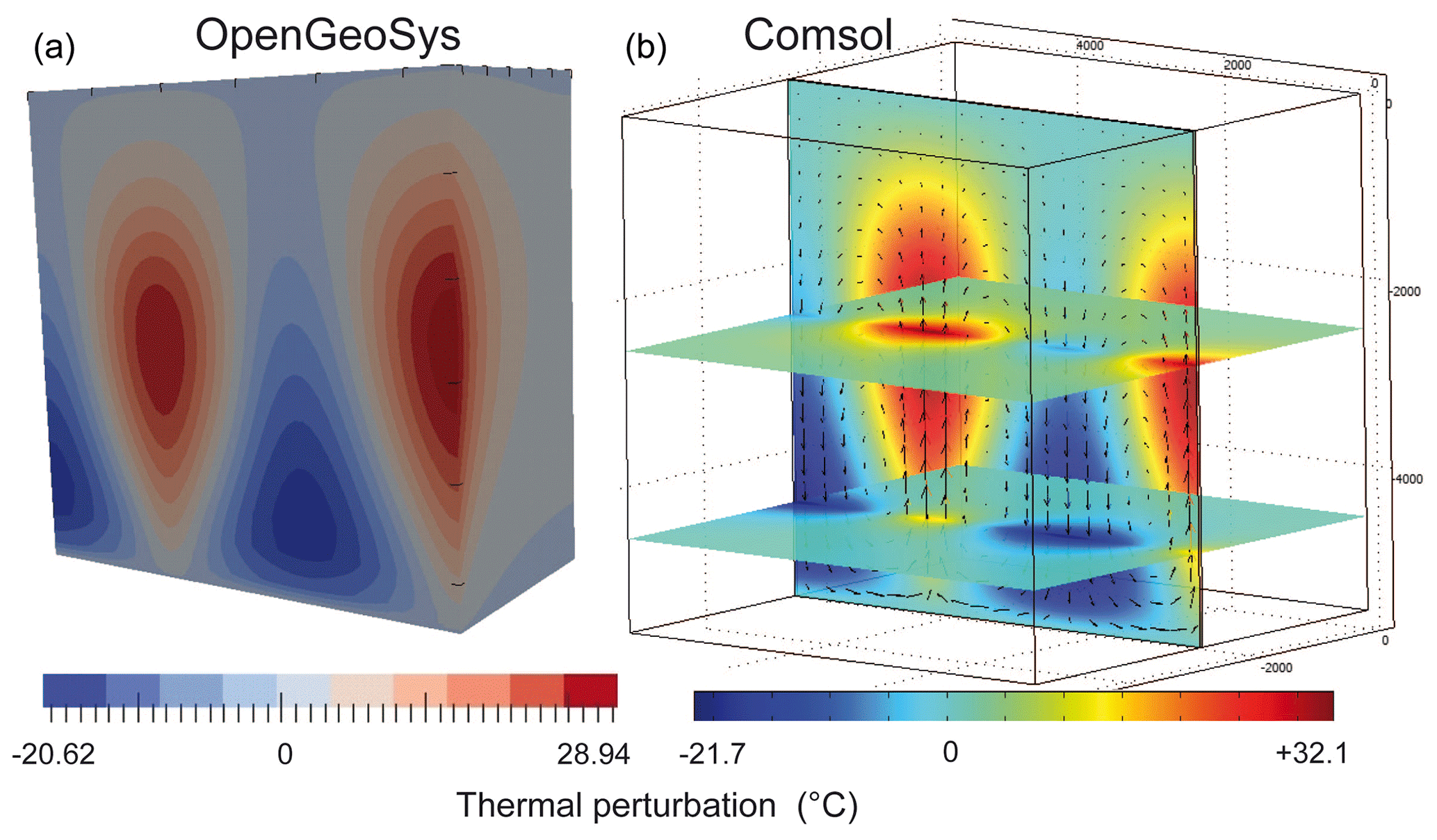
Figure B1 Benchmark experiment for a 40 m wide fault zone embedded in impervious host rock (cube of 5.5 km), as in the Magri et al. (2017) study (a). Our result (b) indicates slight differences in temperature perturbation (see text), but the convective pattern is identical.

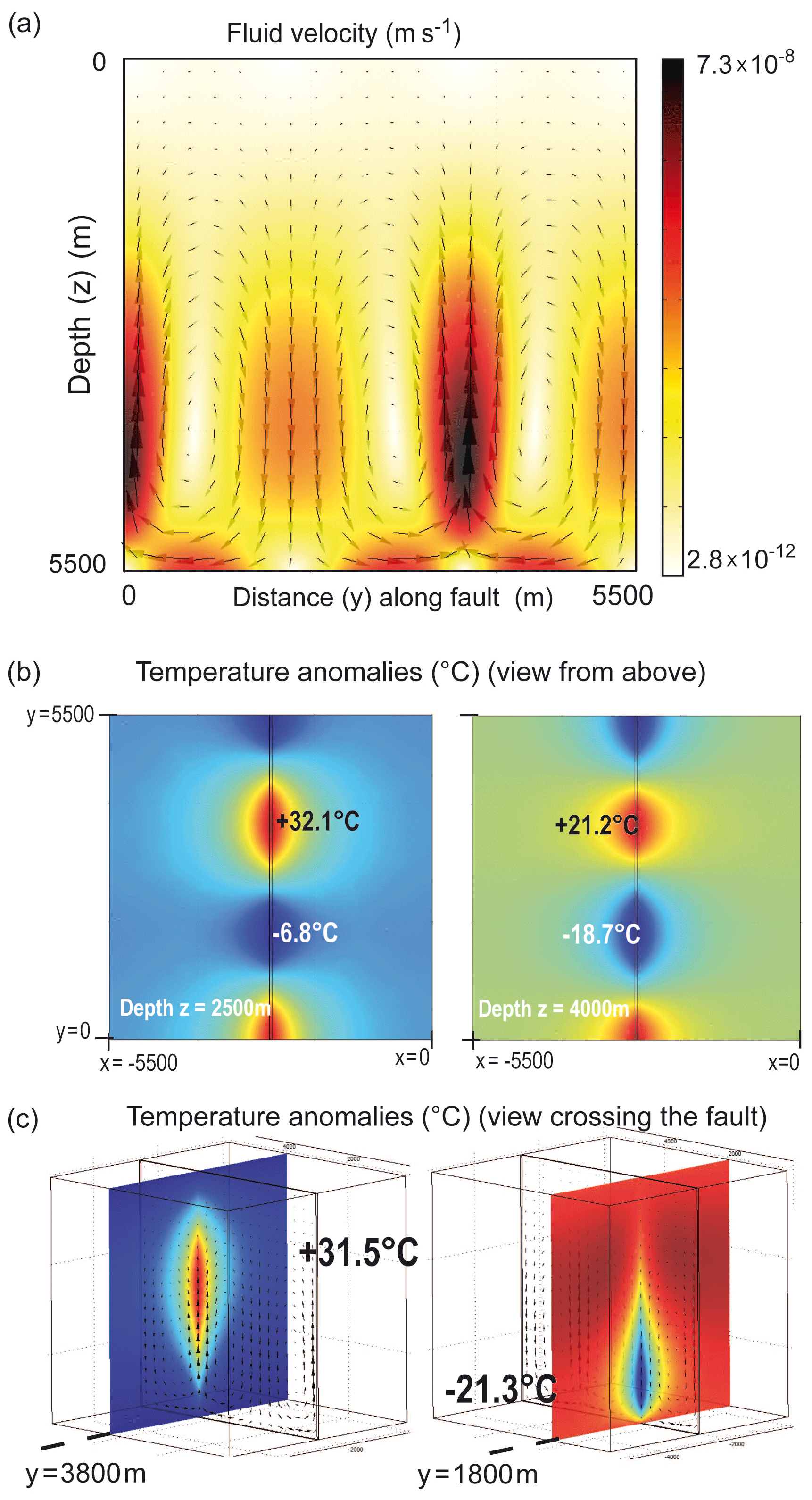
Figure B2 Details of the 3D benchmark experiment in Fig. B1. (a) Field velocity and values within the fault; (b) lateral diffusion of temperature anomalies at depths of 2500 and 4000 m; (c) lateral diffusion of hot and cold anomalies perpendicular to the fault.

Figure B1 shows the 3D benchmark experiment performed with OpenGeoSys (panel a; Fabien Magri, personal communication, 2019) and with Comsol Multiphysics™ (our study; panel b). All boundary conditions are the same, and geometries are identical (fault width is 40 m). The results shown in Fig. B1 correspond to time t₀+10¹³ s. Convective patterns are identical, but temperature anomalies differ by 1 and 3 ^∘C for minimum and maximum values, respectively. As explained by Magri et al. (2017), numerical instabilities may easily develop in density-driven flow problems. In addition, the time discretization adopted by Comsol Multiphysics™ may also differ from that imposed in the other numerical codes.

Figure B2 illustrates some additional details of the convective regime within the fault. The fluid velocity pattern is shown in Fig. B2a, temperature anomalies viewed from above at different depths are shown in Fig. B2b, and temperature anomalies from sections perpendicular to the fault are shown in Fig. B2c. Interestingly, despite the fault width being small (40 m), thermal anomalies diffuse over hundreds of meters (and even thousands of meters if values different from the conductive regime are accounted for).