Estimating ocean tide loading displacements with GPS and GLONASS

Ground displacements due to ocean tide loading have previously been successfully observed using Global Positioning System (GPS) data, and such estimates for the principal lunar M₂ constituent have been used to infer the rheology and structure of the asthenosphere. The GPS orbital repeat period is close to that of several other major tidal constituents (K₁, K₂, S₂); thus, GPS estimates of ground displacement at these frequencies are subject to GPS systematic errors. We assess the addition of GLONASS (GLObal NAvigation Satellite System) to increase the accuracy and reliability of eight major ocean tide loading constituents: four semi-diurnal (M₂, S₂, N₂, K₂) and four diurnal constituents (K₁, O₁, P₁, Q₁). We revisit a previous GPS study, focusing on 21 sites in the UK and western Europe, expanding it with an assessment of GLONASS and GPS+GLONASS estimates. In the region, both GPS and GLONASS data have been abundant since 2010.0. We therefore focus on the period 2010.0–2014.0, a span considered long enough to reliably estimate the major constituents. Data were processed with a kinematic precise point positioning (PPP) strategy to produce site coordinate time series for each of three different modes: GPS, GLONASS and GPS+GLONASS. The GPS solution with ambiguities resolved was used as a baseline for performance assessment of the additional modes. GPS+GLONASS shows very close agreement with ambiguity resolved GPS for lunar constituents (M₂, N₂, O₁, Q₁) but with substantial differences for solar-related constituents (S₂, K₂, K₁, P₁), with solutions including GLONASS being generally closer to model estimates. While no single constellation mode performs best for all constituents and components, we propose to use a combination of constellation modes to recover tidal parameters: GPS+GLONASS for most constituents, except for K₂ and K₁ where GLONASS (north and up) and GPS with ambiguities resolved (east) perform best.

1 Introduction

Earth's gravitational interactions with the Sun and the Moon generate solid Earth and ocean tides. These tides produce periodic variations in both the gravity field and Earth's surface displacement. Additionally, the ocean tides produce a secondary deformational effect due to associated periodic water mass redistribution, known as ocean tide loading (OTL) (e.g. Agnew, 2015; Jentzsch, 1997; Baker, 1984). OTL is observable in surface displacements (and their spatial gradients, i.e. tilt and strain) and gravity. Displacement and gravity attenuate approximately as the inverse of the distance from the point load, while gradients have this relation but with distance squared (Baker, 1984). Thus, OTL displacement and gravity changes show greater sensitivity to regional solid Earth structure in comparison to tilt or strain observations (Martens et al., 2016), making this an observation of interest for studying solid Earth rheology.

Global Navigation Satellite Systems (GNSS) are particularly convenient for measuring OTL displacements due to the widescale deployment of dense instrument arrays. Data from continuous GNSS stations have been shown to provide estimates of OTL with submillimetre precision using two main approaches as described by Penna et al. (2015): the harmonic parameter estimation approach – OTL displacement parameters are solved for within a static GNSS solution (e.g. Schenewerk et al., 2001; Allinson, 2004; King et al., 2005; Thomas et al., 2006; Yuan and Chao, 2012; Yuan et al., 2013); and the kinematic approach – OTL constituents are predominantly estimated from high-rate kinematic GNSS-derived time series (e.g. Khan and Tscherning, 2001; King, 2006; Penna et al., 2015; Martens et al., 2016; Wang et al., 2020). In this paper, we follow the kinematic approach.

To date, GNSS-derived OTL displacements have been estimated using predominantly the US Global Positioning System (GPS). GPS-derived measurements of Earth-surface displacement at tidal periods have been successfully used to observe OTL displacement and validate ocean tide models (Urschl et al., 2005; King et al., 2005). The residual displacement between observed and predicted OTL has been related to deficiencies in ocean tide models, reference-frame inconsistencies, Earth model inaccuracies, the unmodelled constituents’ dissipation effect and systematic errors in GPS (e.g. Thomas et al., 2006; Ito and Simons, 2011; Yuan et al., 2013; Bos et al., 2015).

Recent studies have made use of GPS-derived OTL to study dissipation or anelastic dispersion effects in the shallow asthenosphere at the M₂ frequency (e.g. Bos et al., 2015). This type of investigation has not been easily done previously due to various limiting factors such as the accuracy of ocean tide models and the quality and availability of GPS observations. Recently, however, models have improved dramatically with the use of satellite altimetry (Stammer et al., 2014), and GNSS networks have both expanded and have improved data quality. Together, this has enabled the exploration of limitations in the global seismic Preliminary Reference Earth Model (PREM) (Dziewonski and Anderson, 1981) with GPS observations in the western United States (Ito and Simons, 2011; Yuan and Chao, 2012), western Europe (Bos et al., 2015), South America (Martens et al., 2016), the East China Sea region (Wang et al., 2020) and globally (Yuan et al., 2013). These limitations are associated partially with the incompatibility of the elastic parameters within the seismic (1 s period) and the tidal frequency bands and the anelasticity of the upper layers of the Earth, particularly the asthenosphere. The latter was studied through modelling the GPS-observed residuals of the major lunar tidal constituent, M₂, by Bos et al. (2015) and later Wang et al. (2020), while Lau et al. (2017) used M₂ residual from the global study of Yuan et al. (2013) to constrain Earth's deep-mantle buoyancy.

Previous studies have highlighted an apparently large error in solar-related constituents estimated from GPS, in particular K₂ and K₁. This is in part due to their closeness to the GPS orbital (K₂) and constellation (K₁) repeat periods, which strongly aliases with orbital errors. The closeness to the GPS constellation repeat period may induce interference from other signals such as site multipath which will repeat with this same characteristic period (Schenewerk et al., 2001; Urschl et al., 2005; Thomas et al., 2006). Additionally, the P₁ constituent has a period close to that of 24 h, which is the time span used for the International GNSS Service (IGS)-standard orbit and clock products (Griffiths and Ray, 2009), and hence may be contaminated by day-to-day discontinuities present in the products (Ito and Simons, 2011).

Urschl et al. (2005) proposed that the addition of GLONASS (GLObal NAvigation Satellite System), a GNSS developed and maintained by Russia (USSR before 1991), could improve the extraction of K₂ and K₁ constituents as the orbit period of the GLONASS satellites (∼11 h 15 min 44 s) and constellation repeat period (∼8 d) are well separated from major tidal frequencies. However, for many years, GLONASS suffered from an unstable satellite constellation and very sparse network of continuous observing stations. This has been progressively addressed over the last decade to the point where many national networks now include a high density of GLONASS (and other GNSS) receivers.

We seek to improve estimates of OTL displacement from continuous GNSS data, especially for constituents that are subject to systematic error in GPS-only solutions (e.g. S₂, K₂, K₁, P₁) as found in previous studies (Allinson, 2004; King, 2006; Yuan and Chao, 2012). We do this by using both GLONASS and GPS data to estimate amplitudes and phases for the eight major OTL constituents (M₂, S₂, N₂, K₂, K₁, O₁, P₁, Q₁). As in the very recent study of Abbaszadeh et al. (2020), our work focuses particularly on understanding the sensitivity of estimates to different processing choices, although our work focuses on quite dense network in western Europe, while their work focused on a globally distributed set of stations.

2 Dataset

The sites used in our study are shown in Fig. 1, with a focus on south-west England where a large M₂ OTL signal is present. Of the 21 stations, 14 stations are in south-west England: covering both sides of the Bristol Channel (ANLX, SWAS, CARI, CAMO, PADT, APPL, TAUT) and northern coast of the English Channel up to Herstmonceux (PMTH, PRAE, EXMO, PBIL, POOL, CHIO, SANO, HERT) with one site (BRST) in the south. Two sites are in northern England (WEAR, LOFT) and two in Scotland (LERI, BRAE), with one site in central Europe (ZIM2). All sites are equipped with GPS+GLONASS receivers. Note that sites CAMO, LERI and ZIM2 sites replace CAMB, LERW and ZIMM, respectively, which were used by Penna et al. (2015), to allow use of GLONASS data recorded at the former set of sites.

Aside from the addition of GLONASS data, an important difference to the study of Penna et al. (2015) is the shift in time period from 2007.0–2013.0 to 2010.0–2014.0. This shift provides sufficient GLONASS data following the upgrade of many receivers to track GLONASS from 2009 that followed the restoration of the GLONASS constellation that was finished in March 2010 (24 satellite vehicles; SVs). Despite this covering a shorter time span, the length of continuous observations at each site (minimum availability of 95 % through the dataset) exceeds the recommended ∼1000 d of continuous observations (4 years with 70 % availability) (Penna et al., 2015). The selected time period is fully covered by a complete and homogeneous set of reprocessed orbit and clock products.

The chosen sites experience a range of M₂ up OTL amplitudes from >30 mm (ANLX, APPL, BRST, CAMO, PADT, PRAE), 15–30 mm (CARI, EXMO, LOFT, PBIL, SWAS, TAUT) and <15 mm (BRAE, CHIO, LERI, POOL, SANO, WEAR, ZIM2).

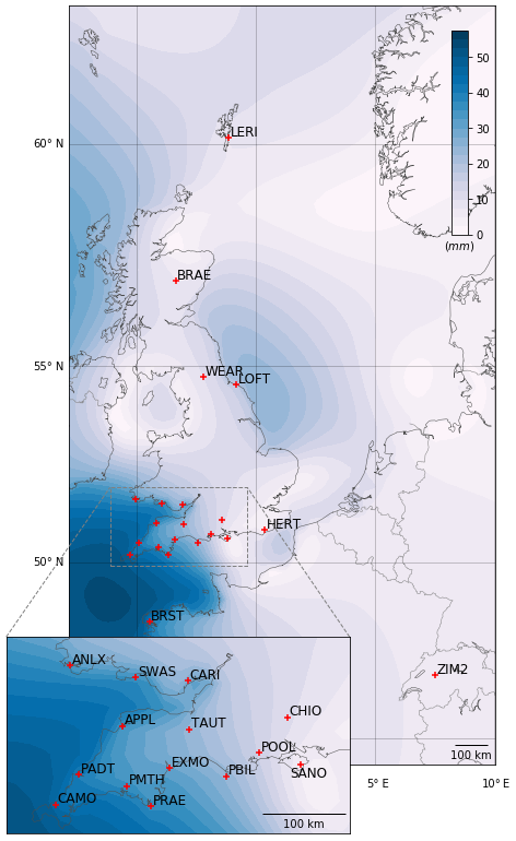
Figure 1 Map of the study area with GNSS site codes and M₂ up displacement amplitude in the background (TPXO7.2 ocean tide model and spherically symmetric Earth with PREM structure).

3 GNSS data processing strategy

The processing strategy was largely based on the GPS-only kinematic precise point positioning (PPP) approach (Zumberge et al., 1997) as per Penna et al. (2015) but with important modifications in terms of the software and to permit the inclusion of GLONASS data. We address PPP in three different modes here: GPS, GLONASS and combined GPS+GLONASS. In particular, we use NASA JPL's GipsyX (v1.3), which is a substantial rewrite of the now legacy GIPSY-OASIS code to allow for, amongst other things, multi-GNSS analysis. Penna et al. (2015) used GIPSY-OASIS v6.1.2. We adopted a PPP solution approach and estimated station positions every 5 min with a random walk model introducing estimated optimum between-epoch constraints on coordinate evolution. We used the VMF1 gridded troposphere mapping function, based on the European Centre for Medium-Range Weather Forecasts (ECMWF) numerical weather model (Boehm et al., 2006). Additionally, ECMWF values for the hydrostatic zenith delay and wet zenith delay were used as a priori values for stochastic estimation of the wet zenith delay as a random walk process with optimum process noise values (Sect. 4) and tropospheric gradients were estimated as a random walk process (Bar-Sever et al., 1998), with process noise at 0.005 mm/sqrt(s) (millimetres per square root second). An elevation cutoff angle of 7 ^∘ was applied, sufficient to maximize the number of GLONASS observations at the respective site latitude as noted by Abbaszadeh et al. (2020), together with observation weights that were a function of the square root of the sine of the satellite elevation angle.

Earth body tide (EBT) and pole tides were modelled according to International Earth Rotation and Reference Systems Service (IERS) 2010 Conventions (Petit and Luzum, 2010). The OTL displacement within each processing run was modelled with the FES2004 tidal atlas (Lyard et al., 2006) and elastic Green functions based on the Gutenberg–Bullen Earth model (Farrell, 1972) (referred to as FES2004_GBe), with centre-of-mass correction applied depending on the adopted orbit products. The FES2004-based OTL values were computed using the free ocean tide loading provider that uses OLFG/OLMP software (http://holt.oso.chalmers.se/loading, last access: 1 October 2020), while the rest of OTL values used in this publication were computed with CARGA software (Bos and Baker, 2005). We did not model atmospheric S₂ tidal displacements.

PPP requires precomputed precise satellite orbit and clock products for each constellation processed, which should be solved for simultaneously within a single product's solution. Unfortunately, JPL's native clock and orbit products are not yet available for non-GPS constellations; hence, we adopted products from two IGS (Johnston et al., 2017) analysis centres (ACs): the European Space Agency (ESA) and Centre for Orbit Determination in Europe (CODE). The ESA combined GPS+GLONASS products from the IGS second reprocessing campaign (repro2) were used (Griffiths, 2019), while CODE's more recent REPRO_2015 campaign (Susnik et al., 2016) had to be used as CODE's repro2 is lacking separate 5 min GLONASS clocks.

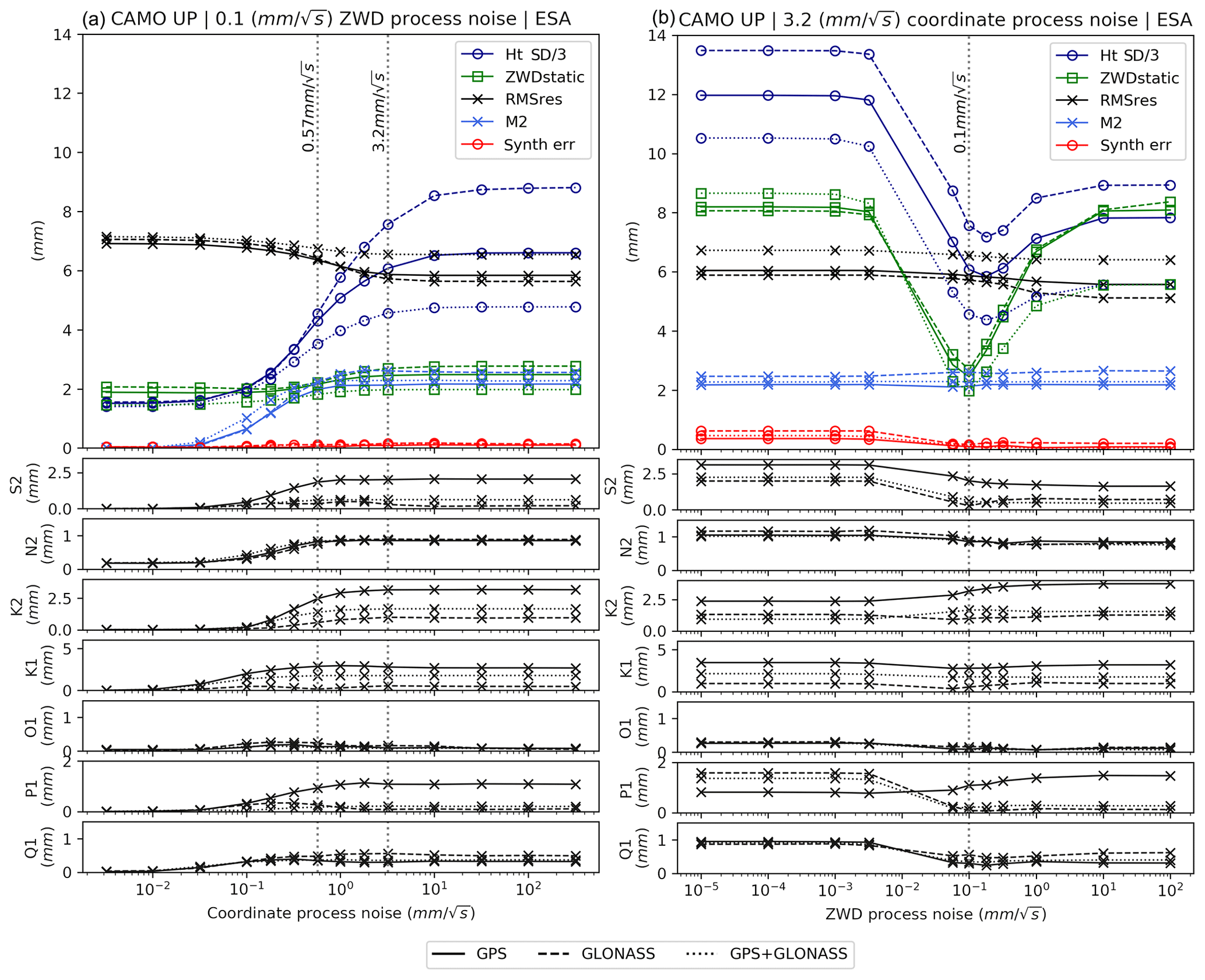
Figure 2 The effect of varying coordinate process noise (a) and zenith wet delay (ZWD) process noise (b) at test site CAMO for the up component (2010.0–2014.0), performed with ESA repro2 products. $\Vert Z_{\text{res}}\Vert$ is relative to FES2004_GBe. The different constellations’ configurations: GPS, GLONASS and GPS+GLONASS are presented as solid, dashed and dotted lines, respectively. The colours pertain to the different metrics as described in the text and legend (note the same scheme is used as per Penna et al., 2015).

All three products consist of satellite orbits and clocks, sampled at 15 and 5 min, respectively, that were held fixed during our processing. The benefit of using JPL's native products, even though solely GPS, is the ability to perform PPP processing with integer ambiguity resolution (AR). PPP AR in GIPSY-OASIS/GipsyX software packages can be performed by using wide lane and phase bias tables which are part of JPL's native products (Bertiger et al., 2010). To provide comparison with previous studies, GPS was processed with JPL's native orbit and clock products from the repro2 campaign (JPL's internal name is repro2.1) with AR.

The CODE and ESA clock and orbit products were generated in different ways. CODE's REPRO_2015 orbit positions were computed using a 3 d data arc, while ESA used a 24 h data arc (Griffiths, 2019). Both ACs provided orbits in a terrestrial reference frame, namely IGS08 and IGb08, respectively, that are corrected for the centre-of-mass (geocentre) motion associated with OTL (FES2004 centre-of-mass correction) and are in the CE frame, following Fu et al. (2012). Alternatively, JPL products were generated from a 30 h data arc and were computed with stations in a near-instantaneous frame realization; hence, the orbits are in the CM frame (we note that the JPL products distributed by the IGS are, by contrast, in CE). Considering the above, the modelled OTL values for JPL's native products solutions were corrected for the effect of geocentre motion, while ESA/CODE products do not require this correction (Kouba, 2009).

It has been suggested that orbit arc length for a given product could potentially impact the estimated OTL displacements. In particular, Ito and Simons (2011) suggest that a 24 h data arc length (as per ESA products) may affect the P₁ constituent due to similarity of the periods. This is in addition to day-boundary edge effects given analysis of data in 24 h batches. We mitigate these effects to some extent by processing the ground stations in 30 h batches (allowing 3 h either side of the nominal 24 h day boundary).

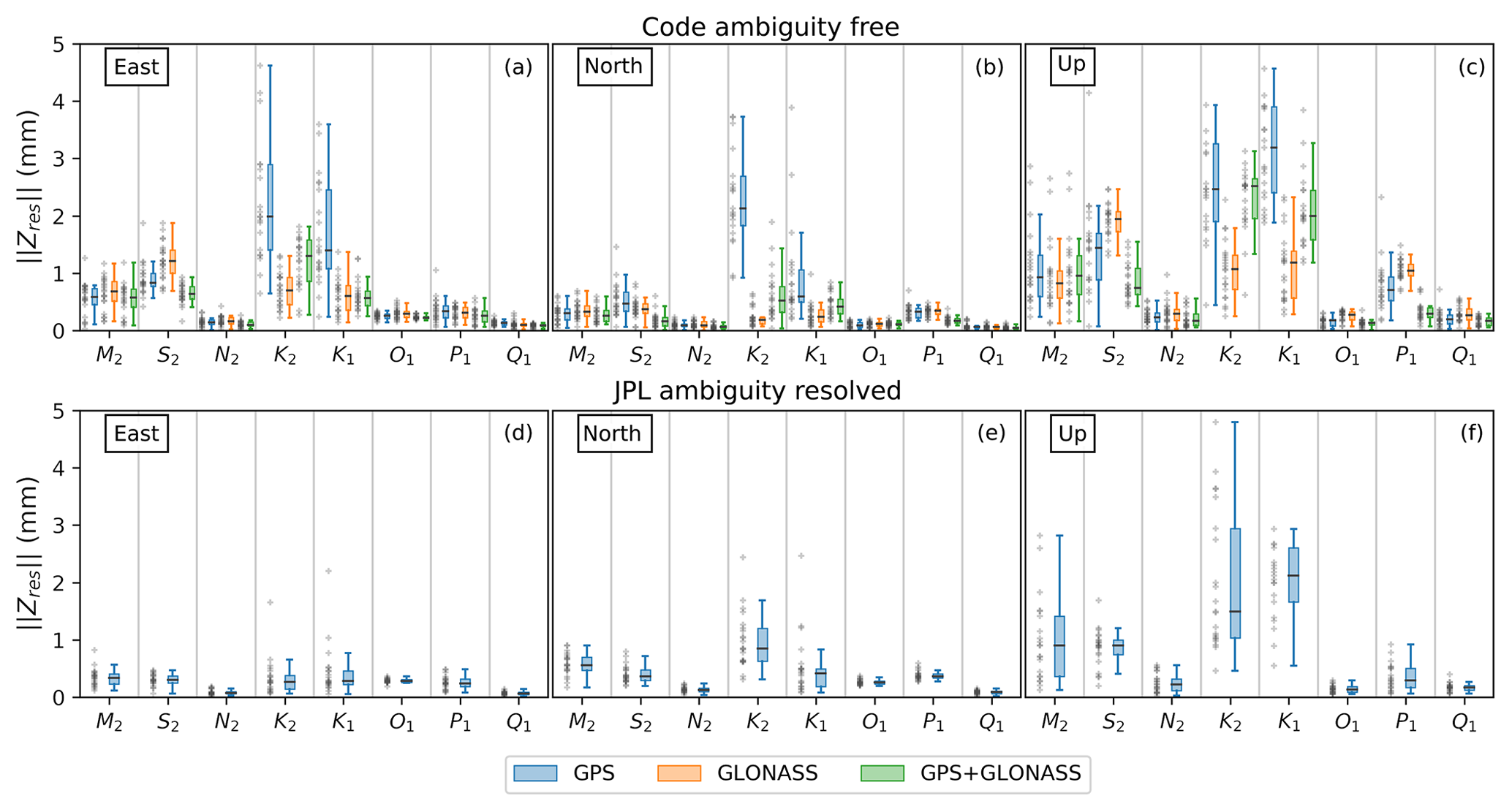
Figure 3 $\Vert Z_{\text{res}}\Vert$ per tidal constituent for east, north and up components (left, middle and right, respectively) relative to FES2014b_STW105d OTL values with centre-of-mass correction (CMC) for JPL solutions. Grey crosses to the left of each boxplot represent sites’ $\Vert Z_{\text{res}}\Vert$ values and are offset horizontally for clarity, while the horizontal line over each boxplot is a median of each constituent's $\Vert Z_{\text{res}}\Vert$. (a–c) $\Vert Z_{\text{res}}\Vert$ for GPS, GLONASS and GPS+GLONASS PPP solutions (blue, orange and green, respectively) computed using CODE products. (d–f) $\Vert Z_{\text{res}}\Vert$ of the GPS AR solution computed with JPL native products. The boxes show the interquartile range and the whiskers mark the limit of an additional $\pm \mathrm{1.5}\times \text{IQR}$, with the median as a horizontal line.

We post-processed the estimated coordinate time series as per Penna et al. (2015): the resulting 5 min sampled solutions were clipped to the respective 24 h window and merged together. Outliers were filtered from the raw 4-year time series using two consecutive outlier-detection strategies: rejecting epochs with extreme receiver clock bias values ($>\mathrm{3}\times {\mathrm{10}}^{\mathrm{3}}$ m) or where the XYZ σ was over 0.1 m and then rejecting epochs with residuals to a linear trend larger than 3 standard deviations per coordinate component. The XYZ time series were converted to a local east–north–up coordinate frame, detrended and resampled to 30 min sampling rate via a simple seven-point window average (seven samples – > one sample). The 30 min averaging reduces high-frequency noise (unrelated to OTL) as well as the computational burden of further harmonic analysis.

Finally, OTL displacements modelled in GipsyX were added back using HARDISP (Petit and Luzum, 2010). HARDISP uses spline interpolation of the tidal admittance of 11 major constituents to infer values of 342 tidal constituents and generate a time series of tidal displacements. This approach almost eliminates the effect of companion constituents (Foreman and Henry, 1989) as they are modelled during the processing stage; small errors in the modelled major OTL constituents will propagate into negligible errors in modelled companion tides. Thus, the analysed harmonic displacement parameters represent true displacement plus an indiscernible companion constituent error that is far below the measurement error. We tested the effect of the “remove–restore” OTL procedure we adopted by solutions without modelling OTL in GipsyX. The resulting differences in M₂ amplitudes were smaller than 0.1 mm, and this was reduced further when coordinate process noise was increased. This confirms that the results are independent of the prior FES2004_GBe OTL values. The findings in our paper are provided in the context of GipsyX software, and solutions derived using other software may produce different results especially if the underlying model choices differ.

The harmonic analysis of the reconstructed OTL signal was performed using ETERNA software v.3.30 (Wenzel, 1996), resulting in amplitudes and local tidal potential phase lags negative which are suitable for solid Earth tide studies. OTL phase lag, however, is defined with respect to the Greenwich meridian and phase lags are positive. Transforming to Greenwich-relative lags was done according to Boy et al. (2003) and Bos (2000). We then computed the vector difference between the reconstructed observed OTL and that predicted by the model, following the notation of Yuan et al. (2013):

$$\begin{array}{}\text{(1)}& Z_{\text{res}}=Z_{\text{obs}}-Z_{\mathrm{th}}.\end{array}$$

In Eq. (1), we assume body tide errors to be negligible; thus, Z_obs is simply an observed OTL and Z_th is a theoretical OTL, while Z_res, the residual OTL, is their vector difference. Z_res presented in this publication is, if not otherwise specified, relative to the theoretical OTL values computed using the FES2014b ocean tide atlas, a successor of FES2012 used in Bos et al. (2015), and a Green function based on the STW105 Earth model additionally corrected for dissipation at the M₂ frequency which we call STW105d (referred to as FES2014b_STW105d). We utilize box-and-whisker plots to visualize the distribution of the estimates with the box and whiskers defined as the interquartile range (IQR) and an additional $\pm \mathrm{1.5}\times \text{IQR}$, respectively, with the median as a horizontal line.

4 Process noise optimization

Process noise settings within GipsyX need to be chosen to ensure optimal separation of site displacement, tropospheric zenith delays, noise, etc. For example, a tight coordinate process noise value, even the default value of 0.57 mm/sqrt(s), tends to clip OTL amplitudes, especially in coastal sites. Penna et al. (2015) developed a method of tuning process noise values for GPS PPP, which we expanded to accommodate the additional major diurnal/semi-diurnal constituents considered here, as well as the use of both GPS and GLONASS data.

To do this, we used the CAMO site, the successor of CAMB used by Penna et al. (2015), and tested a range of coordinate and zenith wet delay (ZWD) process noise settings exactly as described by Penna et al. (2015). We perform separate tests for GPS only, GLONASS only and GPS+GLONASS solutions. These tests focus on a range of metrics, namely the standard deviation of the height time series (shown as “Ht SD/3”, as divided by 3), the standard deviation of kinematic ZWD normalized by ZWD values from a static solution (“ZWDstatic”), root mean square of the carrier phase residuals (“RMSres”), M₂ residual OTL magnitude, $\Vert Z_{\text{res}}\Vert$, and $\Vert Z_{\text{res}}\Vert$ of a synthetic ∼13.96 h signal and its controlled, known input (designated “Synth err”). We focus on the results without the introduction of this synthetic signal here.

For each of the major constituents, both diurnal and semi-diurnal, and for each of the constellation choices, we found that 3.2 mm/sqrt(s) for coordinate process noise and 0.1 mm/sqrt(s) for tropospheric zenith delay process noise were optimal for our solutions, the same values as identified by Penna et al. (2015) for M₂ using GPS only. Figure 2 shows the results of the tests, with Fig. 2a showing the result of varying coordinate process noise, while ZWD process noise was held fixed (0.1 mm/sqrt(s), a default value) and Fig. 2b the result of varying the ZWD process noise with coordinate process noise equal to the optimum value of 3.2 mm/sqrt(s). The finding of identical optimal process noise settings for all constituents and constellations suggests that the different amplitudes and frequencies are less important than the data noise in the semi-diurnal and diurnal frequency bands and that the constellation-specific data noise does not substantially vary between constellations.

5 Results and discussion

Given the known accuracy of the ocean tide models in this region (Penna et al., 2015), and small effects of errors in solid Earth models, our assumption is that as $\Vert Z_{\text{res}}\Vert$ approaches zero, the estimates increase in accuracy, also shown by Bos et al. (2015). Based on previous studies (e.g. Yuan et al., 2013), we expected $\Vert Z_{\text{res}}\Vert$ median values (up component) of ∼2 mm for K₂ and K₁, ∼1 mm for M₂, S₂ and P₁, and ∼0.5 mm for N₂, O₁ and Q₁.

Figure 3a–c show GPS, GLONASS and GPS+GLONASS $\Vert Z_{\text{res}}\Vert$ estimates for each of the east, north and up coordinate components. Over all components, the $\Vert Z_{\text{res}}\Vert$ are uniformly small for N₂, O₁ and Q₁, with median around 0.1 mm. Residuals are slightly higher for M₂, P₁ and S₂, with the median being around 0.5–0.7 mm, and are often noticeably higher for K₁ and K₂, although there is substantial variation by constellation.

The combined GPS+GLONASS solutions perform either at the same level as GPS AR (M₂, O₁, Q₁) or better (N₂, P₁) for the up component. $\Vert Z_{\text{res}}\Vert$ values are smaller and more consistent for the east (M₂, N₂, O₁) and north (M₂, N₂, P₁) components, respectively. The GPS+GLONASS solution does not have $\Vert Z_{\text{res}}\Vert$ biases in the east and north components as is noticeable for the GPS AR solution (particularly for O₁ in the east and P₁ in the north, respectively). By $\Vert Z_{\text{res}}\Vert$ bias, we mean a noticeable gap between zero and the lower whisker.

Considering the problematic GPS K₂ and K₁ constituents, the GPS AR can reasonably reliably, in comparison to other types of solutions, extract $\Vert Z_{\text{res}}\Vert$ in the east component (Fig. 3d) which is smaller than that of GLONASS and GPS+GLONASS using ESA or CODE products. However, the smallest $\Vert Z_{\text{res}}\Vert$ in the up and north components is possible only using the GLONASS constellation solely which aligns with the conclusions of Abbaszadeh et al. (2020), who used ESA products and globally distributed GNSS network of sites.

Our results suggest that no single solution provides consistently better constituent estimates across all coordinate components. We suggest that optimum results are obtained using GPS+GLONASS for M₂, S₂, N₂, O₁, P₁ and Q₁, and GLONASS for K₂ and K₁, noting that GPS AR performs better for all constituents in the east component.

We now explore the sensitivity of our solutions to different products and analysis choices starting with elevation cutoff angle sensitivity, which particularly affects the amount of multipath influence on the coordinate time series. We pay particular attention to S₂, K₂, P₁ and K₁ given the large systematic errors evident in GPS-only solutions. We follow with an intercomparison of solutions using various products and then assess the impact of integer ambiguity resolution (GPS only). Finally, we test the stability of the constituent estimates to time series length.

5.1 Satellite orbit and clock product sensitivity tests

We assessed whether the solutions were sensitive to changes in satellite-elevation cutoff angle. Three additional cutoff angle scenarios were tested: 10^∘, 15^∘ and 20^∘ (in addition to the default 7^∘ cutoff angle). Different elevation angle cutoffs will significantly alter the observation geometry as well as modulate the expression of signal multipath into solutions, decreasing the likely influence of multipath with higher cutoff values.

Figure 4a–c show the magnitude of vector difference, $\Vert \mathrm{\Delta }{Z}_{\text{res}}\Vert$, between Z_res values estimated from the 7^∘ and 20^∘ solutions and CODE products in both cases. S₂, K₂, K₁ and P₁ constituents in the up coordinate component show larger mean magnitudes of vector differences in both GPS (0.56, 2.29, 2.88 and 0.54 mm, respectively) and GLONASS (0.82, 0.64, 1.01 and 0.58 mm, respectively) with the rest of constituents showing differences of less than 0.5 mm. GPS+GLONASS shows the smallest $\Vert \mathrm{\Delta }{Z}_{\text{res}}\Vert$ between 7^∘ and 20^∘ cutoff estimates for S₂ and P₁ (0.31 and 0.23 mm, respectively) and an additional decrease in $\Vert \mathrm{\Delta }{Z}_{\text{res}}\Vert$ for M₂, S₂,N₂, O₁ and Q₁ in the up component. The high agreement between OTL values indicates the high stability of GPS+GLONASS estimates with changing cutoff angles.

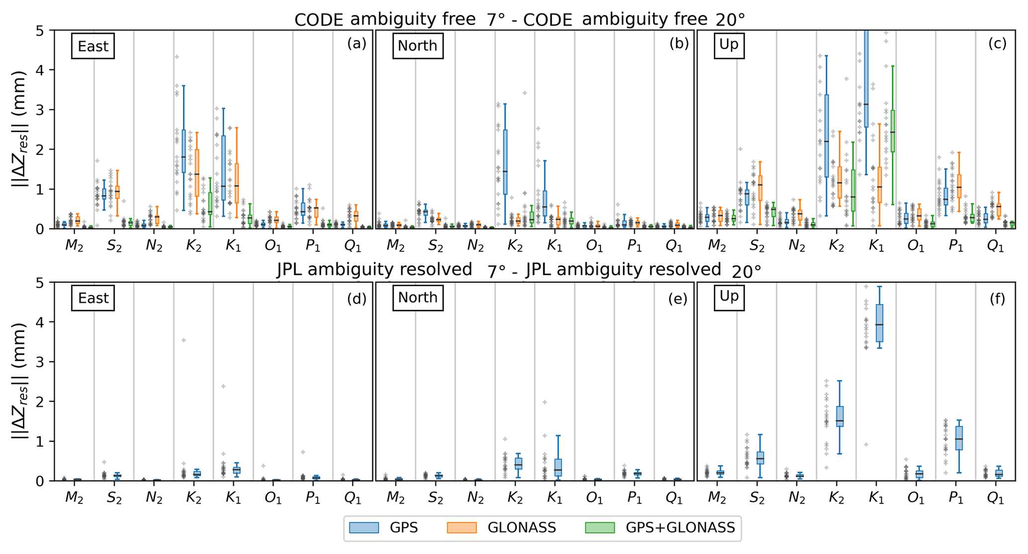
Figure 4 Magnitude of vector difference between estimated Z_res values computed with 7^∘ and 20^∘ elevation cutoff angles, $\Vert \mathrm{\Delta }{Z}_{\text{res}}\Vert$, within the same set of orbits and clocks (a–c CODE; d–f JPL AR) for east, north and up coordinate components (left, middle and right, respectively). Grey crosses are as per Fig. 3. The smaller residuals using CODE products with GPS+GLONASS (a–c) are a result of improved OTL stability as a function of cutoff angle using combined constellations (except K₁ up and K₂ up). JPL's GPS AR also shows great stability, with the exception of K₂ up and K₁ up. $\Vert \mathrm{\Delta }{Z}_{\text{res}}\Vert$ for GPS, GLONASS and GPS+GLONASS PPP solutions is in blue, orange and green, respectively.

The same comparison for GPS AR (7^∘ and 20^∘ cutoff, JPL native products) shows largely improved stability in comparison to all GPS-only ambiguity-free solutions (Fig. 4d–f). However, K₂ up and K₁ up show substantial differences between solutions: K₂ shows as much smaller variance of $\Vert Z_{\text{res}}\Vert$ distribution in the 20^∘ solution, possibly due to removal of multipath, and K₁ shows an increased variance and median of $\Vert Z_{\text{res}}\Vert$ at increased cutoff angle.

Following Yuan et al. (2013), we assessed the possible influence of inconsistencies in precomputed orbits or clocks on estimated OTL displacements. This was done by computing $\Vert \mathrm{\Delta }{Z}_{\text{res}}\Vert$ between pairs of solutions with common constellation configurations: GPS (no AR here) solutions computed using ESA, CODE and JPL products; GLONASS/GPS+GLONASS solutions using ESA and CODE products. Figure 5a–c show the distribution of $\Vert \mathrm{\Delta }{Z}_{\text{res}}\Vert$ between solutions computed with ESA and CODE products for all three constellation modes: GPS, GLONASS and GPS+GLONASS. The main differences are related to the S₂, K₂, K₁ and P₁ constituents. The maximum $\Vert \mathrm{\Delta }{Z}_{\text{res}}\Vert$ between the observed OTL for the rest of the constituents is less than ∼0.3 mm.

Compared with GPS JPL, both CODE and ESA solutions (Fig. 5d–f and g–i, respectively) show $\Vert \mathrm{\Delta }{Z}_{\text{res}}\Vert$ up to 0.5 mm in the horizontal components with respect to JPL solutions, which is also true for ESA in the up component with the exception of K₂ and K₁. CODE shows similar behaviour to ESA; however, significant divergence from JPL (Fig. 5d–f) is also observed for S₂ with even higher $\Vert \mathrm{\Delta }{Z}_{\text{res}}\Vert$ for K₂ and K₁ in the up and the east.

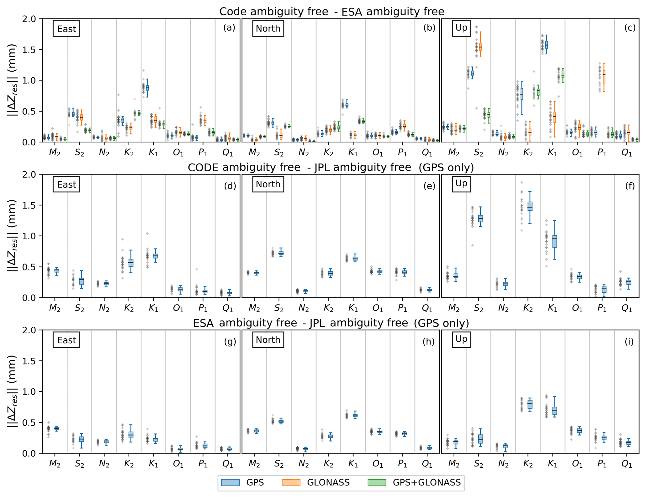
Figure 5 OTL vector differences between CODE, ESA and JPL solutions (ambiguity free). (a–c) GPS, GLONASS and combined GPS+GLONASS differences between CODE and ESA solutions; (d–f) GPS difference between CODE and JPL solutions (ambiguity free); (g–i) GPS difference between ESA and JPL solutions (ambiguity free). Note the vertical scale of 2 mm. Grey crosses are as per Fig. 3.

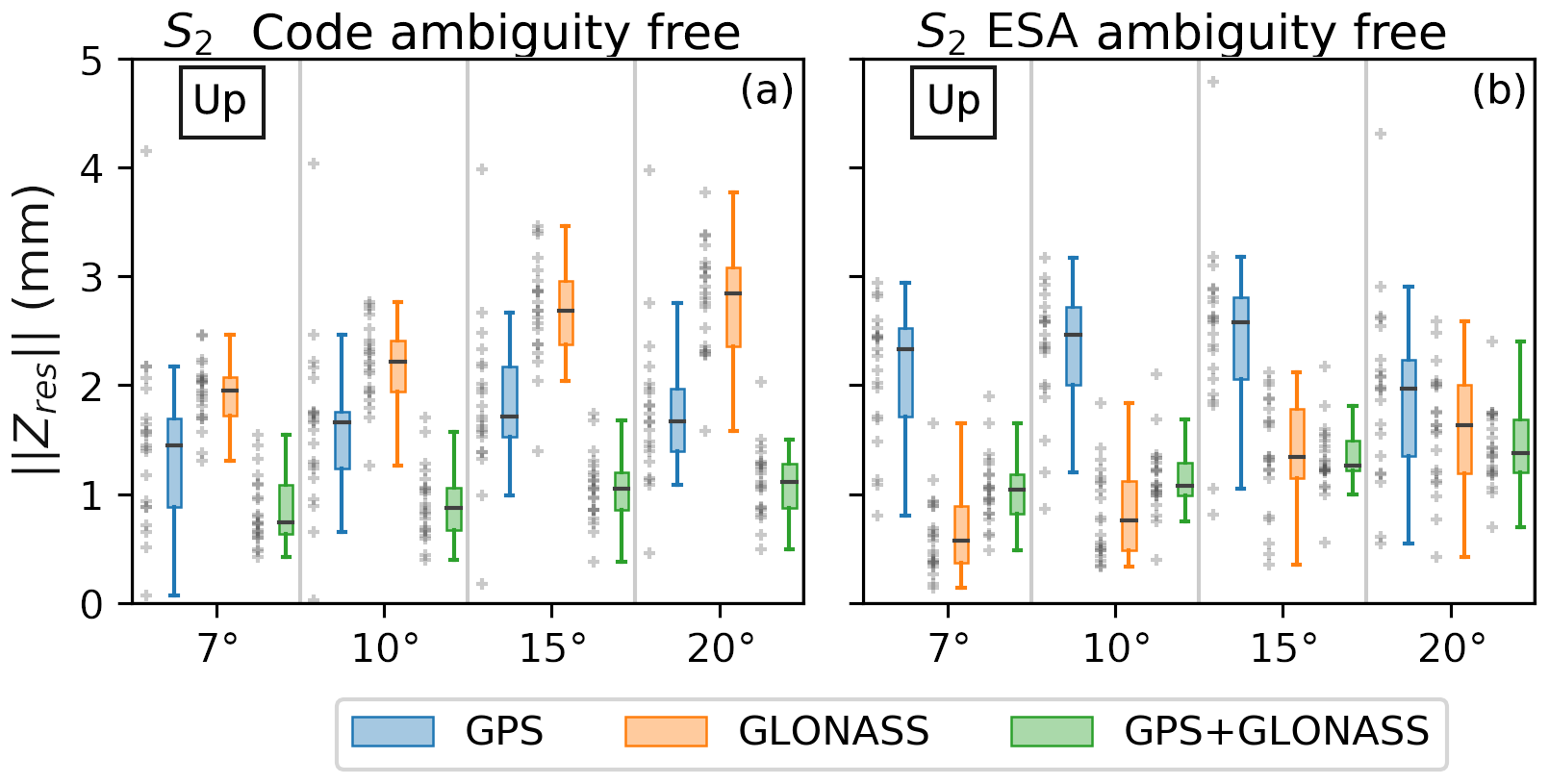
Figure 6 GPS, GLONASS and GPS+GLONASS $\Vert Z_{\text{res}}\Vert$ for the S₂ constituent in the up component as a function of elevation cutoff angle, computed with ESA (a) and CODE products (b). Note the inverse behaviour of GPS and GLONASS biases and the linear dependence of the GLONASS biases. Grey crosses are as per Fig. 3.

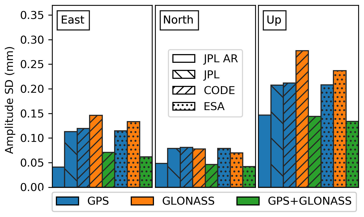
Figure 7 Average uncertainties (1σ) for OTL amplitudes computed across eight OTL constituents per products (stipple) and processing modes or constellation (colour): GLONASS (orange) and GPS (blue) modes show higher 1σ uncertainties, while GPS-only AR and combined GPS+GLONASS (green) show minimum 1σ uncertainties with the exception of east.

5.2 S₂ constituent

Focusing on S₂, the GPS up residual shows ∼1 mm residual bias between solutions using CODE and ESA products (compare blue records between Fig. 6a and b). The GPS $\Vert Z_{\text{res}}\Vert$ bias remains for solutions with a range of elevation cutoff angles (7^∘, 10^∘, 15^∘ and 20^∘). GLONASS solutions (orange), however, show no $\Vert Z_{\text{res}}\Vert$ bias for ESA and ∼1.5 mm bias for CODE, both with 7^∘ elevation angle. GLONASS bias values with both products increase with elevation cutoff angle up to 15^∘. This GLONASS dependency with elevation cutoff is present to a lesser degree in both east and north components and is the same with ESA and CODE products (Fig. S5).

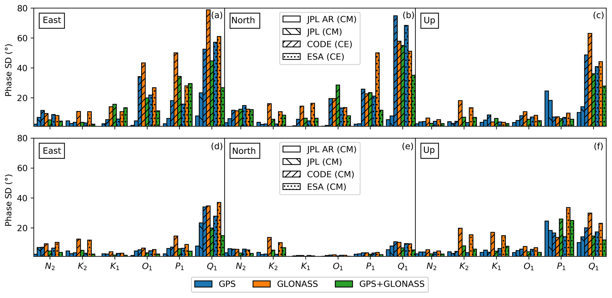
Figure 8 Average phase uncertainty per constituent for different products as returned by ETERNA. ESA and CODE products were in CE frame by default (a–c) and converted to CM (d–f), while JPL products are in CM in both. M₂ and S₂ phase 1σ uncertainties are not shown here as values are too small to be seen with the scale specified.

GPS $\Vert Z_{\text{res}}\Vert$ estimates show similar behaviour in terms of $\Vert Z_{\text{res}}\Vert$ bias between ESA and CODE solutions in the up component (blue, Fig. 6) but ESA solutions' median $\Vert Z_{\text{res}}\Vert$ values are ∼1 mm larger for all elevation cutoff angle solutions. Both ESA and CODE GPS+GLONASS S₂ results (green, Fig. 6) show a blend of the two patterns observed with GPS and GLONASS solutions. GPS+GLONASS S₂ shows less sensitivity to the cutoff angle change than GLONASS or GPS solutions alone.

The substantial difference in S₂ between ESA and CODE (Fig. 6) suggests important differences in raw GNSS data analysis approaches within respective ACs. One relevant difference between products is in treatment of S₁ and S₂ atmospheric tides which were corrected for at the observation level in CODE products but not in ESA. However, the inverse behaviour of GPS and GLONASS between ESA and CODE solutions (orange, Fig. 6) cannot be explained with a single correction applied to both constellations. We expect that the differences in each solution are a function of satellite orbit modelling, although the exact origin is not clear and needs further investigation.

5.3 K₂ and K₁ constituents

As seen from Fig. 3, $\Vert Z_{\text{res}}\Vert$ can be minimized if using GLONASS for the extraction of K₁ and K₂ constituents and GPS+GLONASS for the remainder of the constituents. In this case, $\Vert Z_{\text{res}}\Vert$ will stay below 0.25 mm for north components and below 0.5 mm for the east and the up components.

GLONASS K₂ and K₁ estimates in the north have the lowest variance in $\Vert Z_{\text{res}}\Vert$ and are most stable with different elevation cutoff angles and products. For the east component, CODE products with GLONASS have larger $\Vert Z_{\text{res}}\Vert$ median and scatter than with GPS+GLONASS for K₁ and in terms of elevation cutoff stability (K₂ and K₁). Solutions using the ESA GLONASS products, however, perform better for K₁ east than the respective GPS+GLONASS in terms of $\Vert Z_{\text{res}}\Vert$ distribution consistency and median (Fig. S2). Elevation cutoff stability of ESA K₂ and K₁ in the east component is best with GPS+GLONASS as also found when using CODE products.

The up component of K₂ and K₁ is the most problematic, showing high $\Vert Z_{\text{res}}\Vert$ values with all constellation modes. GLONASS OTL values using either both ESA or CODE products have the smallest medians and variances of $\Vert Z_{\text{res}}\Vert$, outperforming JPL GPS AR. Note that GPS+GLONASS K₂ up has a marginally smaller median $\Vert \mathrm{\Delta }{Z}_{\text{res}}\Vert$ in the elevation cutoff test than that of GLONASS only, possibly due to the larger number of total satellites; however, both K₂ and K₁ $\Vert Z_{\text{res}}\Vert$ suggest a ∼1.5 mm bias.

While we cannot definitively select a single constellation configuration optimal for all components of K₂ and K₁, we can conclude that based on our analysis, GLONASS solutions have smaller $\Vert Z_{\text{res}}\Vert$ in the K₂ and K₁ north and up components, while the east component shows better results with GPS+GLONASS (K₁, CODE). However, we recommend GLONASS-only solutions due to the higher level of agreement between solutions using ESA and CODE products. The only exception is the east component, where the preference is for JPL GPS AR (see Sect. 5.7).

5.4 P₁ constituent

GLONASS P₁ constituents show high $\Vert \mathrm{\Delta }{Z}_{\text{res}}\Vert$ between CODE and ESA solutions over all coordinate components (orange, Fig. 5a–c). This was unexpected as ESA and CODE $\Vert Z_{\text{res}}\Vert$ boxplots show similar distributions of values (see Fig. S2 in the Supplement for the equivalent ESA boxplots). This suggests a symmetrical deviation from the modelled values that produces a high $\Vert \mathrm{\Delta }{Z}_{\text{res}}\Vert$. In all cases, however, GPS+GLONASS is preferred for P₁ estimation.

5.5 Effect of different orbit and clock products on noise and uncertainty

Changing orbit and clock products also changes the time series noise characteristics and hence influences the uncertainties of the estimated constituents (estimated separately by ETERNA for amplitude in Fig. 7 and phase in Fig. 8). Amplitude uncertainties are expressed here as an average across all constituents, as they do not differ much between analysed constituents. ETERNA assumes a white noise model in its analysis. We conclude that GLONASS solutions produce the highest amplitude uncertainties for east (0.15 mm CODE, 0.14 mm ESA) and up components (0.22 mm CODE, 0.27 mm ESA), while showing the same uncertainty as GPS for the north (0.07 mm, both CODE and ESA). GLONASS solutions using CODE products tend to have amplitude uncertainties that are marginally higher than those of ESA products. The amplitude uncertainties for combined GPS+GLONASS solutions are equal to those of JPL with ambiguities fixed (GPS AR), although the JPL GPS AR solution has slightly smaller uncertainty in the east component (smaller by ∼0.02 mm).

Considering the uncertainties of phase values, these are unsurprisingly dependent on the constituent's amplitude. Because JPL native products are in a CM frame, the constituent amplitudes are larger at the time of ETERNA analysis than those using ESA and CODE products which are both provided in a CE frame. For the ESA and CODE solution, this results in up to an order of magnitude increase in phase uncertainties for “weaker” diurnal constituents in the region: N₂, O₁, P₁, Q₁ (Fig. 8).

In general, this frame effect is directly related to centre-of-mass correction (CMC) specific to the constituent's CMC vector in comparison to the total theoretical OTL vector. If applying a CMC correction to the constituent increases its amplitude, phase SD values will decrease in a CM frame solution. This is critically important for the constituents with amplitudes below 0.5 mm, as phase uncertainty increases significantly below this threshold. The most significant exception in our dataset is P₁ in the up component, which has a much larger amplitude in CE frame (Fig. 8c and f).

Converting CE products to CM (Fig. 8d–f) was done to demonstrate that the changes in phase uncertainty are indeed introduced by the smaller amplitudes in the CE frame. While this holds true, it is obvious that the P₁ up phase uncertainty increases, as was expected based on comparison with the JPL solutions. GLONASS K₁ up phase uncertainties show almost an order of magnitude increase in the CM frame while having unexpectedly small values in CE. This is a direct cause of GLONASS solution having larger K₁ up amplitudes in CE and smaller in CM with both CODE and ESA.

5.6 Impact of ambiguity resolution on GPS

The multi-GNSS products used here do not allow integer AR with PPP, and this is an active area of research and development within the IGS. However, assessing the impact of AR on GPS-only solutions provides some insight towards the future benefit of AR on GLONASS and GPS+GLONASS solutions once such products become available. We compared OTL residuals from GPS and GPS AR using JPL native products that contain wide lane and phase bias tables (WLPB files) required for integer AR with PPP.

Figure 9 shows the effect on estimated constituents from enabling AR in a standard solution with 7^∘ cutoff. Here, we observe decreased $\Vert Z_{\text{res}}\Vert$ over all coordinate components compared with the estimates from a non-AR solution. This is most visible in the K₂ and K₁ constituents and in the elimination of the S₂ $\Vert Z_{\text{res}}\Vert$ bias and with smaller improvements in M₂ and P₁.

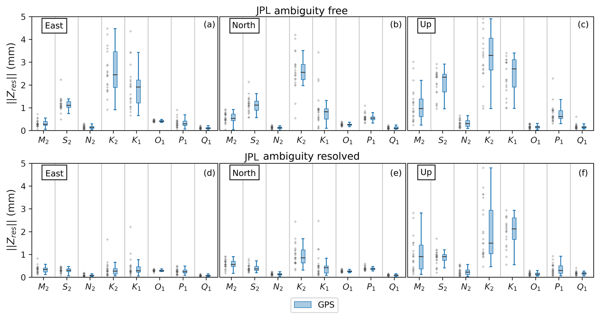
Figure 9 Comparison of residual constituents' estimates from GPS (a–c) and GPS AR (d–f) JPL native solutions. Grey crosses are as per Fig. 3. As seen, most of constituents’ $\Vert Z_{\text{res}}\Vert$ distribution variances and medians are smaller, while S₂ $\Vert Z_{\text{res}}\Vert$ bias is removed with AR solutions.

Importantly, Fig. 9 shows that enabling AR eliminates $\Vert Z_{\text{res}}\Vert$ bias in GPS and aligns the residual vectors with ESA/CODE GPS+GLONASS (Fig. 3). This is a clearer improvement than reported by Thomas et al. (2006).

Given this effect, the S₂ $\Vert Z_{\text{res}}\Vert$ bias was once again assessed with various elevation cutoff angles solutions. JPL GPS solutions (floating AR), in the up component (Fig. 10a), show the S₂ $\Vert Z_{\text{res}}\Vert$ bias to be constant with cutoff angle, being about 1 mm, and with the $\Vert Z_{\text{res}}\Vert$ variance of around 3 mm. Similar behaviour was previously observed with solutions using ESA products (Fig. 6).

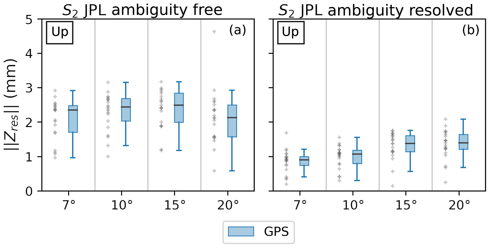
Figure 10 GPS S₂ up constituent's $\Vert Z_{\text{res}}\Vert$ change with elevation cutoff angle computed with JPL products floating AR (a) and integer AR (b). Grey crosses are as per Fig. 3. As seen, AR helps in removing the bias and decreases the $\Vert Z_{\text{res}}\Vert$ distribution variance.

Enabling integer ambiguity resolution (GPS AR) removes the ∼1 mm S₂ $\Vert Z_{\text{res}}\Vert$ bias completely at 7^∘ and 10^∘ elevation cutoff angles while leaving ∼0.4 mm bias at 15^∘ and 20^∘ in the up component. Consequently, up $\Vert Z_{\text{res}}\Vert$ medians change by 1–2 mm depending on elevation cutoff angle. Based on this observation, we expect that resolving ambiguities within PPP might help in solving, or at least minimizing, the S₂ $\Vert Z_{\text{res}}\Vert$ present in ESA GPS and CODE GLONASS solutions. Eliminating biases in GPS and GLONASS separately should increase the stability and consistency of GPS+GLONASS S₂ $\Vert Z_{\text{res}}\Vert$.

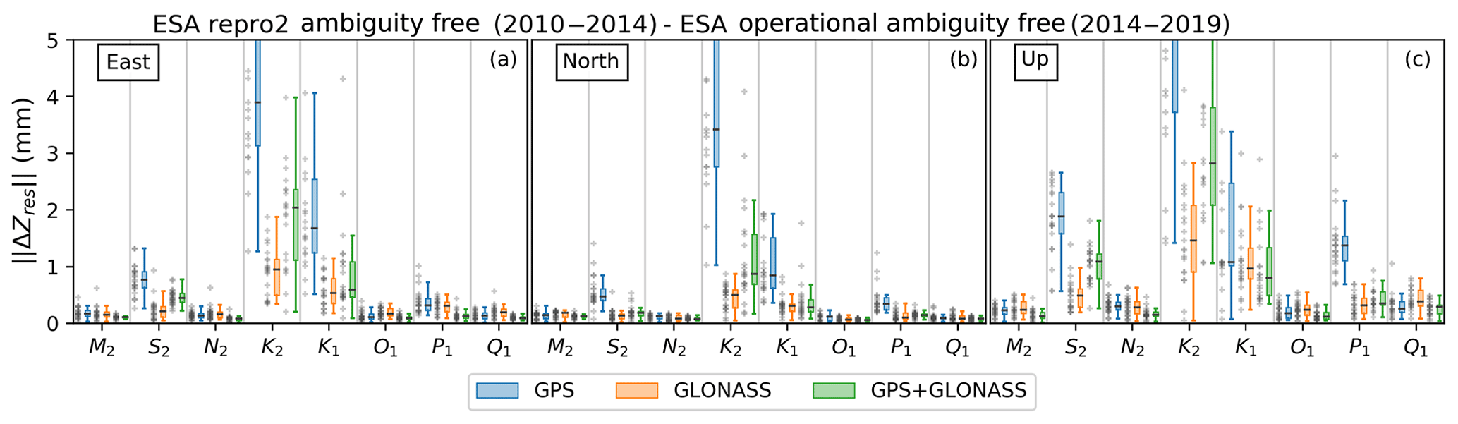
Figure 11 OTL vector differences between ESA repro2 (2010.0–2014.0) and ESA operational (2014.0–2019.0) OTL estimates: GPS (blue), GLONASS (orange) and GPS+GLONASS (green) constellation modes present. Grey crosses are as per Fig. 3.

5.7 Impact of time series length

Yuan et al. (2013) used a filter-based harmonic parameter estimation approach and examined the dependence of Kalman filter convergence on time series length for each of the eight major constituents. Yuan et al. (2013) concluded that, after 1000 daily solutions, convergence (minimized $\Vert Z_{\text{res}}\Vert$) was reached for lunar-only constituents (M₂, N₂, O₁, Q₁), while reporting solar-related constituents (S₂, K₂, K₁, P₁) were not fully converged even after 3000 daily solutions.

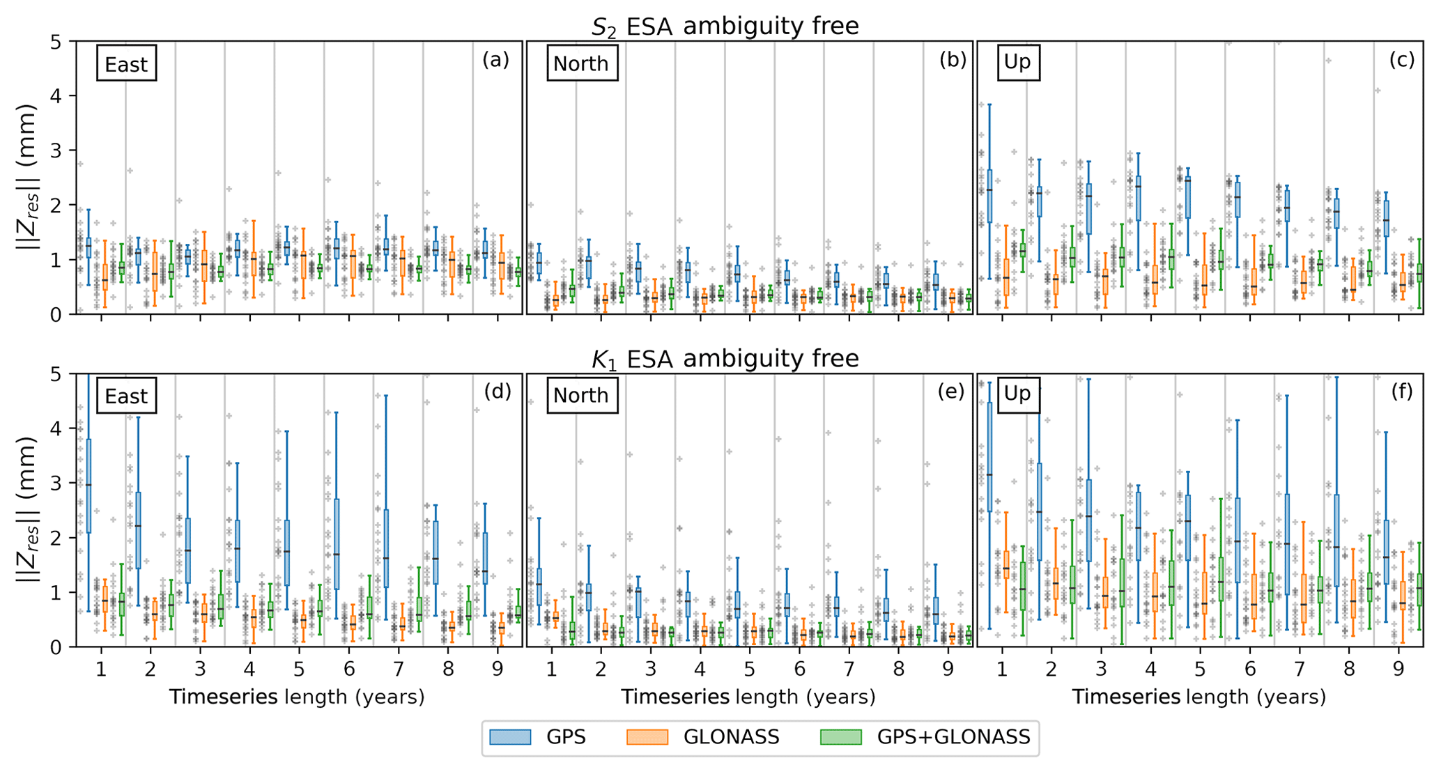
Figure 12 Dependency of estimated $\Vert Z_{\text{res}}\Vert$ and time series' length in years for two solar-related constituents: S₂ (a–c) and K₁ (d–f). GPS, GLONASS and GPS+GLONASS PPP solutions are in blue, orange and green, respectively, using ESA products. Grey crosses are as per Fig. 3. Note that 1–4 years of time series length use ESA repro2, while the rest use a combination of ESA repro2 and ESA operational products.

We assessed how $\Vert Z_{\text{res}}\Vert$ of each of eight major constituents varies as a function of the time series length with kinematic estimation approach. The duration of the series varied by integer years and, to enable a complete analysis, we expanded the candidate solutions to 2019.0 and processed additional data with operational products: JPL repro3.0, ESA operational, CODE MGEX (CODE operational lacks GLONASS clock corrections). While the goal of a reprocessing campaign is to preserve consistency with operational products (Griffiths, 2019), based on previous results, we assumed that changing satellite orbit and clock products may produce substantial differences in problematic solar-related constituents (S₂, K₂, K₁, P₁). Thus, we first performed a comparison of ESA repro2 solutions (2010.0–2014.0) with the ESA operational product (2014.0–2019.0) which confirmed the hypothesis (Fig. 11). GLONASS $\Vert \mathrm{\Delta }{Z}_{\text{res}}\Vert$ show the smallest variance for K₁ and K₂ compared with GPS and GPS+GLONASS but are significant, up particularly, which might be related to the changes in the analysis used to produce GLONASS orbits and clocks. Considering S₂, the very same form of bias remains as previously seen in the 2010.0–2014.0 dataset. This suggests a symmetric deviation of repro2 and operational products solutions from the modelled value. The same explanation can be applied to the GPS-only P₁ $\Vert \mathrm{\Delta }{Z}_{\text{res}}\Vert$ bias in the up component of 0.5 mm.

The results shown in Fig. 12 are produced from a composition of reprocessed products and operational products (years 5 to 9). We focus on S₂ up and K₁ up, as the most problematic diurnal constituents. The results align with general conclusions of Yuan et al. (2013) suggesting a weak relationship between time series length and $\Vert Z_{\text{res}}\Vert$ for solar-related constituents. However, if constituents are examined according to our recommended optimum constellation strategy, $\Vert Z_{\text{res}}\Vert$ appears (see Fig. S4) stable over time, which suggests that even if there are changes in the products, they are not having an impact with this methodology.

6 Conclusions

We expand the GPS-only methodology of ocean tide loading displacement estimation described in Penna et al. (2015) with data from the GLONASS constellation. We assess the performance of GPS and GLONASS for the estimation of eight major ocean tide loading constituents in stand-alone modes and in a combined GPS+GLONASS mode. We examine data from 21 sites from the UK and western Europe over the period of 2010.0–2014.0 through processing data in kinematic PPP using products from three different analysis centres: CODE, ESA and JPL. The latter was also used to assess the effect of GPS ambiguity fixing on estimated ocean tide loading displacements. All solutions were intercompared to gain an insight into the sensitivities of the constituent estimates to different choices of satellite orbit and clock products, satellite elevation cutoff and constellation configurations.

We find that the optimal constellation mode varies across all eight major tidal constituents and components. We show that ambiguity-free GPS+GLONASS solutions show a similar level of precision as GPS with ambiguities resolved (GPS AR), with P₁ estimates using GPS+GLONASS showing improved precision and stability. The K₂ and K₁ constituents, which are known to be problematic in GPS solutions, are still unusable in GPS+GLONASS solutions, presumably due to the propagation of GPS related errors. The S₂ constituent also cannot be reliably recovered with GPS+GLONASS, as GLONASS shows dependency between the estimates and the chosen elevation cutoff angle. GPS-based estimates of S₂ show a constant bias in absolute residuals when ambiguity resolution is not implemented, but this is substantially reduced by resolving the ambiguities to integers. GLONASS-based estimates show a comparable level of performance to ambiguity-free GPS for M₂, N₂, O₁, P₁ and Q₁, while showing improved results for K₂ and K₁.

Additional comparison of OTL estimates from reprocessed and operational products shows that GLONASS estimates of K₂ and K₁ show differences in the up and, to a lesser extent, in the east components when using different products.

Considering the above information, we suggest that estimation of K₁ and K₂ constituents is best undertaken using GLONASS only solutions with an emphasis towards the north component where it is most stable. M₂, S₂, N₂, O₁ and Q₁ can be reliably estimated from combined GPS+GLONASS or GPS AR solutions, while P₁ is best with GPS+GLONASS.

Integer ambiguity resolution was not possible in the GLONASS or GPS+GLONASS solutions tested here due to limitations in the products available. However, evidence from our GPS AR testing suggests that further increases in precision and stability will be seen when AR fixing can be performed using GLONASS, and this should have a positive impact on estimates of solar-related constituents.