the Creative Commons Attribution 4.0 License.
the Creative Commons Attribution 4.0 License.
 | 19 May 2021
Relocation of earthquakes in the southern and eastern Alps (Austria, Italy) recorded by the dense, temporary SWATH-D network using a Markov chain Monte Carlo inversion
Christian Haberland
Trond Ryberg
Vincent F. Verwater
Eline Le Breton
Mark R. Handy
Michael Weber
In this study, we analyzed a large seismological dataset from temporary and permanent networks in the southern and eastern Alps to establish high-precision hypocenters and 1-D VP and models. The waveform data of a subset of local earthquakes with magnitudes in the range of 1–4.2 ML were recorded by the dense, temporary SWATH-D network and selected stations of the AlpArray network between September 2017 and the end of 2018. The first arrival times of P and S waves of earthquakes are determined by a semi-automatic procedure. We applied a Markov chain Monte Carlo inversion method to simultaneously calculate robust hypocenters, a 1-D velocity model, and station corrections without prior assumptions, such as initial velocity models or earthquake locations. A further advantage of this method is the derivation of the model parameter uncertainties and noise levels of the data. The precision estimates of the localization procedure is checked by inverting a synthetic travel time dataset from a complex 3-D velocity model and by using the real stations and earthquakes geometry. The location accuracy is further investigated by a quarry blast test. The average uncertainties of the locations of the earthquakes are below 500 m in their epicenter and ∼ 1.7 km in depth. The earthquake distribution reveals seismicity in the upper crust (0–20 km), which is characterized by pronounced clusters along the Alpine frontal thrust, e.g., the Friuli-Venetia (FV) region, the Giudicarie–Lessini (GL) and Schio-Vicenza domains, the Austroalpine nappes, and the Inntal area. Some seismicity also occurs along the Periadriatic Fault. The general pattern of seismicity reflects head-on convergence of the Adriatic indenter with the Alpine orogenic crust. The seismicity in the FV and GL regions is deeper than the modeled frontal thrusts, which we interpret as indication for southward propagation of the southern Alpine deformation front (blind thrusts).
- Article
(9322 KB) - Full-text XML
-
Supplement
(82 KB) - BibTeX
- EndNote


The Alpine orogen resulted from the collision of the European and Adriatic plates (Dewey et al., 1973; Schmid et al., 2004; Handy et al., 2010, 2015). This collision led to localized deformation patterns within the plates and along the suture, often accompanied by seismic activity. The seismicity of the Alps has been investigated both on the scale of the Alpine orogen (e.g., Diehl, 2008) and on the scale of parts of the chain (e.g., the southern Alps; Amato et al., 1976; Cagnetti and Pasquale., 1979; Galadini et al., 2005; Anselmi et al., 2011; Scafidi et al., 2015; Bressan et al., 2016; Slejko, 2018; Viganò et al., 2008, 2013, 2015). The southern and eastern Alps have heterogeneous earthquake distribution, with regions of high activity, e.g., the eastern southern Alps (ESA); rare activity, e.g., the eastern Alps; or inactivity, e.g., parts of western southern Alps (WSA) (Fig. 1).
The dense temporary seismic SWATH-D network was deployed from 2017 to 2019 in the southern and central Alps (Heit et al., 2017, 2021) with a total number of 161 stations. Given the average station spacing of only 15 km, this network was designed to capture the shallow crustal seismicity (especially the depths of the earthquakes) with higher precision than the coarser permanent networks, including the AlpArray network (AASN, with 52 km station spacing; Hetényi et al., 2018), and to obtain an increased spatial resolution of images (e.g., local earthquake tomography, receiver functions), even in a region with low or moderate local seismicity. The SWATH-D network is located in a key part of the Adriatic indenter, for which a switch in subduction polarity was proposed at the transition from the central to eastern Alps (e.g., Lippitsch et al., 2003).
In this study, we use a subset of 335 local earthquakes recorded by the SWATH-D network and complemented by a selection of 112 AlpArray network stations nearby to precisely relocate the hypocenters of the local earthquakes. The dense, high-quality travel time picks created in this study potentially lead to constrained hypocenter solutions with high internal consistency. This will enable us to identify the general pattern of seismicity on the surface and at depth throughout the region and contribute to the understanding of active tectonic processes. A further aim of the study is to derive a high-quality dataset suitable to be used in local earthquake tomography (LET).
Although locating earthquakes has been a routine task in seismology for decades, there are several challenges related to obtaining a precise location. One of them is the trade-off between the hypocenters and the velocity structure (so-called hypocentre–velocity coupling; Kissling, 1988; Thurber, 1992; Kissling et al., 1994). To yield accurate locations (especially depths), either the velocity model should be well known in advance or, particularly in the case of earthquakes occurring within a network (local earthquakes), it has to be simultaneously inverted for (Kissling, 1988; Kissling et al., 1994; Thurber, 1983; Husen et al., 1999). This is conventionally being done by employing iterative inversion strategies based on damped least squares. These methods are quite robust and have been successfully applied for years. However, because they use a linearization and the damped least-squares approach, they depend not only on proper choices of initial values for hypocenter coordinates (close enough to the true location) and the velocity model(s) but also on model parametrization (i.e., layers) or regularization (i.e., damping factors), which all have to be carefully checked and selected.
Recently, a transdimensional, hierarchical Bayesian approach utilizing a Markov chain Monte Carlo (McMC) algorithm was implemented for simultaneous inversion of hypocenters, 1-D velocity structure, and station corrections, specifically for the local earthquake case (Ryberg and Haberland, 2019). This approach has the advantage of being largely independent of prior knowledge of model parameters (starting velocity model, starting locations of earthquakes), and the inversion results are data-driven. Moreover, the results can be statistically analyzed, and thus errors and ambiguities can be estimated. The method extends the probabilistic relocation approaches (Lomax et al., 2000) by inverting for a set of velocity models well explaining the data.
The study region (Fig. 1) is part of the collisional zone between the Adriatic and European tectonic plates. The convergence of these plates began no later than 84 Ma, with the onset of collision at ca. 35 Ma (Dewey et al., 1973; Schmid et al., 2004; Handy et al., 2010) and culminating since ca. 24 Ma with north-northwestward indentation of the Adriatic continental lithosphere (Handy et al., 2015). Indentation is still ongoing today (Cheloni et al., 2014; Aldersons, 2004; Serpelloni et al., 2016; Sánchez et al., 2018).
Deformation in the target area (red box in Fig. 1) occurred within a corner of the Adriatic indenter, which is delimited to the north by the Periadriatic Fault (PAF) and to the west by the Guidicarie Fault (GF). The PAF is a late orogenic fault active in Oligo–Miocene time, which was sinistrally offset by the GF in Miocene time. Just north of the northwestern corner of the indenter, where the GF and PAF meet, the Tauern Window (TW) exposes remnants of the European lower plate at the surface (Scharf et al., 2013; Schmid et al., 2013; Favaro et al., 2017; Rosenberg et al., 2018). Therefore, shortening and exhumation within the TW are attributed to faulting along the Adriatic indenter (Scharf et al., 2013; Favaro et al., 2017; Reiter et al., 2018). Counterclockwise rotation of the Adriatic plate with respect to the Eurasian plate (Le Breton et al., 2017) is interpreted to have induced seismic activity in the southern Alps (Anderson and Jackson, 1987; Mantovani et al., 1996; Bressan et al., 2016).
The thrust front in the eastern southern Alps (ESA) accommodates most of the Adria–Eurasia convergence with pronounced N-oriented present-day motion (Serpelloni et al., 2016; Sánchez et al., 2018). A N-oriented horizontal deformation of ∼2 mm a−1 is observed in the ESA front (northern part of the Venetian-Friuli Basin; Sánchez et al., 2018; Métois et al., 2015; Cheloni et al., 2014) with highest recorded geodetic strain rate along the Venetian Front (within the Montello region, around 45.8∘ N, 12.25∘ E) (Serpelloni et al., 2016; Verwater et al., 2021). From the Venetian part of ESA toward the Po Basin (PoB), the motion vectors have a slight westward rotation with decreasing magnitudes. In contrast, a progressive eastward rotation of motion vectors is observed from the Venetian area toward the Pannonian Basin. The entire Alpine chain is still undergoing uplift, with a maximum in the inner Alps, e.g., along the border between Switzerland, Austria, and Italy (near 46.6∘ N, 11∘ E) with values of ≥ 2 mm a−1, whereas uplift rates decrease toward the foreland (Sánchez et al., 2018).
Two sedimentary basins, the Molasse and the Po basins (MoB and PoB in Fig. 1) dominate the shallow structure at the northern and southern borders of the target area. The MoB, running along the northern front of the Alps, thickens going across strike from the exposed Variscan basement (0 km) to the Alpine Front (5 km; see, e.g., depth-to-basement contours in the map of Bigi et al., 1989). The Quaternary and Tertiary sediments of the PoB thicken from 0 km at its northern margin to about 6 km in the south below the Apenninic front (Bigi et al., 1989; Waldhauser et al., 2002).
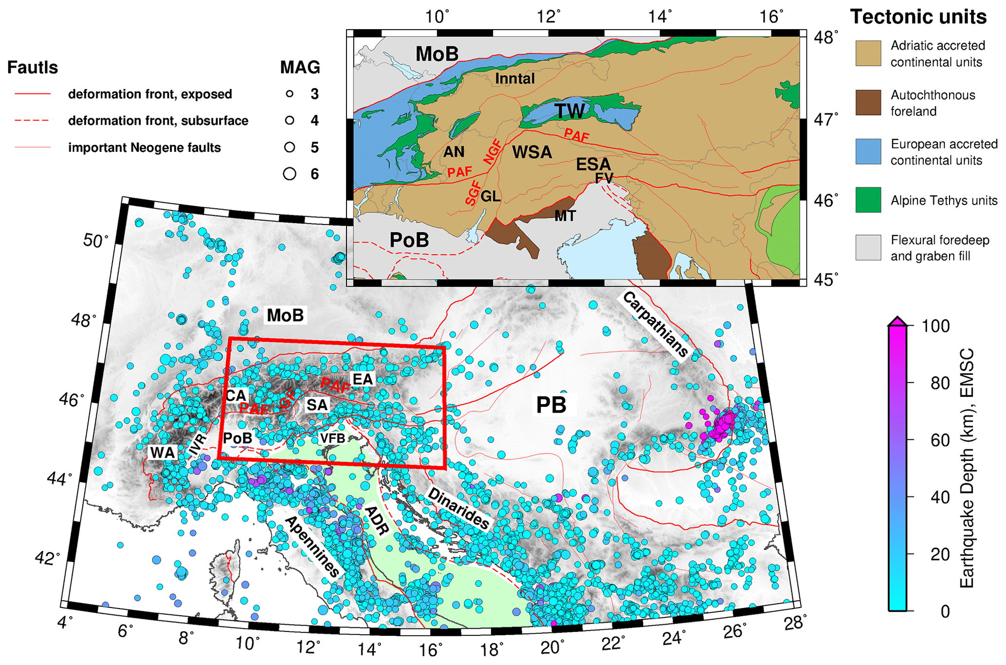
Figure 1Geological map of the Alps showing major deformation fronts, faults, geographical subdivisions, tectonic units, and seismicity (seismic events between January 2000 and December 2012 with a magnitude larger than 3 from the European-Mediterranean Seismological Centre). The light green zone indicates the outline of the Adriatic plate. The tectonic units of the study area (red box) are shown on the upper-right inset map. The maps are modified from Handy et al. (2010) and Schmid et al. (2004, 2008). Abbreviations are as follows: WA stands for western Alps, CA stands for central Alps, SA stands for southern Alps, EA stands for eastern Alps, ADR stands for Adriatic plate, IVR stands for Ivrea body, PB stands for Pannonian Basin, VFB stands for Venetian-Friuli Basin, PoB stands for Po Basin, MoB stands for Molasse Basin, TW stands for Tauern Window, PAF stands for Periadriatic Fault, NGF stands for northern Giudicarie Fault, SGF stands for southern Giudicarie Fault, ESA stands for eastern southern Alps, WSA stands for western southern Alps, MT stands for Montello, GL stands for Giudicarie–Lessini region, FV stands for Friuli-Venetia region, and AN stands for Austroalpine nappes.
The seismicity in the study area and surrounding regions has been monitored routinely for many years with stations operated by different national and regional networks ( National Institute of Geophysics and Volcanology, INGV, and National Institute of Oceanography and Experimental Geophysics, OGS, in Italy; Central Institution for Meteorology and Geodynamics in Austria, ZAMG; and Swiss Seismological Service in Switzerland, SED). Besides routine catalogs, the seismicity has also been investigated in a few seismological studies through various time periods and regions (Blundell et al., 1992; Solarino et al., 1997; Galadini et al., 2005; Diehl, 2008; Viganò et al., 2013; Reiter et al., 2018, among others). Diehl (2008) compiled the local earthquake data from 14 seismic networks in the greater Alpine region from 1996 to 2007 and created a uniform and consistent relocated event catalog. The SHARE European Earthquake Catalog (Grünthal et al., 2013) comprised homogeneous earthquakes from 1000 to 2006.
These studies indicate that seismic activity is clustered in the Friuli-Venetia (FV), Giudicarie–Lessini (GL), and the Inntal regions (Fig. 1). The FV region is located along the thrust-and-fold belt marking the active Adria–Europe plate boundary and was struck by several earthquakes of MW≥6 over the last several centuries (Slejko, 2018). The energy was released on a system of E–W south-verging thrusts (some of which are blind or unknown), as well as on backthrusts and oblique-slip faults (Nussbaum, 2000; Galadini et al., 2005; Slejko, 2018; Romano et al., 2019). The GL region is located in the deformation zone along the western margin of Adriatic indentation with two major fault and fold systems characterized by high seismic activity: the Giudicarie Belt and the Schio-Vicenza strike-slip fault (Viganò et al., 2015). In contrast, the area east of the northern Guidicarie Fault (NGF) has obviously been much less active since at least 1994 (Viganò et al., 2015).
3.1 Network data
For this study, we used mainly data of the SWATH-D network, which was temporarily deployed in a roughly rectangular region in northern Italy and southeastern Austria (black box in Fig. 2). The installation started in Summer 2017, and the network ran for almost 2 years (Heit et al., 2017, 2021). The network consisted of 151 broadband seismometers with an average inter-station spacing of 15 km. A total of 78 stations equipped with Güralp-3ESPC seismometers (https://www.guralp.com/products/surface, last access: 1 November 2020) and Earth Data EDR-210 recorders (http://www.earthdata.co.uk/edr-210.html, last access: 1 November 2020) transmitted data in near real-time via the cellular network (online). The other 73 stations, with data accessed during station services (offline), were equipped with two different kinds of seismometers and digitizers: 58 of them with Nanometrics portable Trillium Compact seismometers (https://www.nanometrics.ca/products/seismometers/trillium-compact, last access: 1 November 2020) and CUBE recorders (https://www.gfz-potsdam.de/en/section/geophysical-deep-sounding/infrastructure/geophysical-instrument-pool-potsdam-gipp/pool-components/seismic-pool/recorder-dss-cube3/, last access: 1 November 2020), and the rest with Güralp-3ESPC seismometers and Earth Data PR6-24 recorders (http://www.earthdata.co.uk/pr6-24.html, last access: 1 November 2020). In Autumn 2018, the network was complemented with an additional 10 online stations in the northeastern edge by LMU-Munich. All SWATH-D seismic stations recorded the data continuously at 100 samples per second (sps).
In order to enlarge the azimuthal coverage for earthquakes occurring in the periphery of the SWATH-D framework, we additionally selected 112 stations of the larger-scale AlpArray Seismic Network (AASN; Hetényi et al., 2018) to include their waveform data in the analysis.
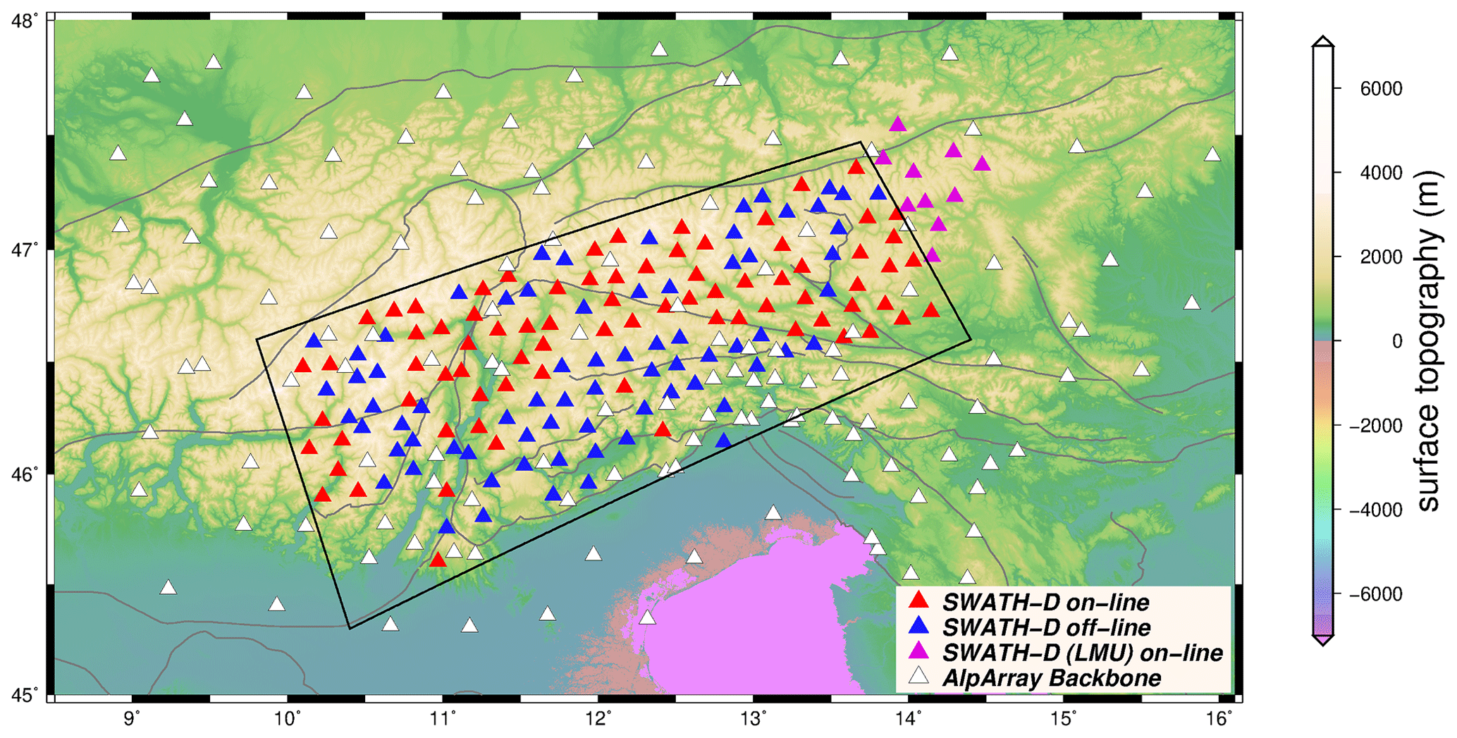
Figure 2Distribution of seismic stations of the SWATH-D network (red, blue, purple) and selected stations of the AASN (white). The black box indicates the periphery of the SWATH-D network. The faults are from Schmid et al. (2004, 2008) and Handy et al. (2010).
3.2 Seismic events, arrival time picks, and phase-type identification
The national seismological agencies of Italy (INGV and OGS), Austria (ZAMG), and Switzerland (SED) provide comprehensive earthquake catalogs (minimum magnitude −0.8 by ZAMG) in our study region. Therefore, the process of event detection was skipped and an integrated event list from the national agencies, after removal of common events, formed a proper list of 2639 local events (see Appendix A for more information) for arrival time picking. Considering this large number of events and 273 selected permanent and temporary stations, we applied a modified version of the automated multi-stage workflow from Sippl et al. (2013) to the waveform data for picking the arrival times of P and S waves. This workflow was originally implemented for producing a complete catalog of well-located earthquakes and reliable arrival times using continuous passive seismic data in the Pamir–Hindu Kush region (Sippl et al., 2013). We, subsequently, assessed the performance of the picking algorithms by quality-checking of time and phase-type uncertainties of the picks (Appendix B).
As described in Sect. B2, the number of mispicks and picks ignored by the automatic procedure was quite large. Therefore, a dataset with relatively highly constrained events was selected for visual (manual) inspection. Since the number of picks in this stage (after the automatic procedure) is not the most reliable information on the location precision (see Sect. B2) and also considering that this data is aimed for high location accuracy of the occurring earthquakes, we selected events with azimuthal gap less than 200∘ and root mean square (rms) less than 1 s, which resulted in 384 event (18 390 P and 7762 S picks). This visual (manual) inspection of this dataset was carried out by removing or modifying obvious mispicks (mainly at large epicentral distances) and also re-picking the missed arrivals (mostly S picks at small epicentral distances).
This manual (visual) inspection was mainly performed on individual station data. The direct Pg (Sg), Moho-reflected PmP (SmS), and Moho-refracted Pn (Sn) phases arrive closely spaced in time, especially in the triplication zone, potentially leading to phase-type misidentification. The PmP (SmS) is always a secondary arrival, but its amplitude can dominate the first arrival and thus be easily mispicked. On the other hand, for epicentral distances larger than the triplication zone, the Pn (Sn) amplitude can be so weak that the Pg (Sg) or PmP (SmS) be wrongly identified as the first arrival. In the local earthquake case, and particularly for regions with varying Moho topography and significant lateral variations in the crustal structure, something to be expected for the Alps, the phase-type identification is even more challenging (Diehl et al., 2009b). Since the inversion is based on the first arrival times we looked at the waveforms in epicentral distance plots for larger events for which we expect the later phases, inspected the picks, and corrected or adjusted where needed. However, we would like to point out that even with these procedures we cannot rule out a certain amount of misidentified phases.
An inspection for identifying potential quarry blasts (and other anthropogenic sources) was simultaneously performed during the visual inspection. Criteria for potential quarry blasts were (1) relatively small number of S-picks, (2) relatively small amplitude ratios (see, e.g., Walter et al., 2018), and (3) large surface waves (observed dispersive waveform characteristics). Based on our assessment, we classified the events into 344 earthquakes, 15 potential blasts, and 25 unclear events.
A Wadati diagram (Wadati, 1933; Kisslinger and Engdahl, 1973; Diehl, 2008) was used to calculate the ratio of the earthquakes, which is 1.72 (calculated by linear least squares; Fig. 3). Furthermore, S picks with S–P travel time differences larger than 4 s off the main trend were removed (however, this was only 0.3 % of all picks). After this removal, only 2 % of the whole observations have s. We notice that at P travel times larger than ∼ 25 s the observations tend to slightly larger S–P travel time differences, potentially indicating a higher ratio at larger depth, i.e., in the upper mantle.
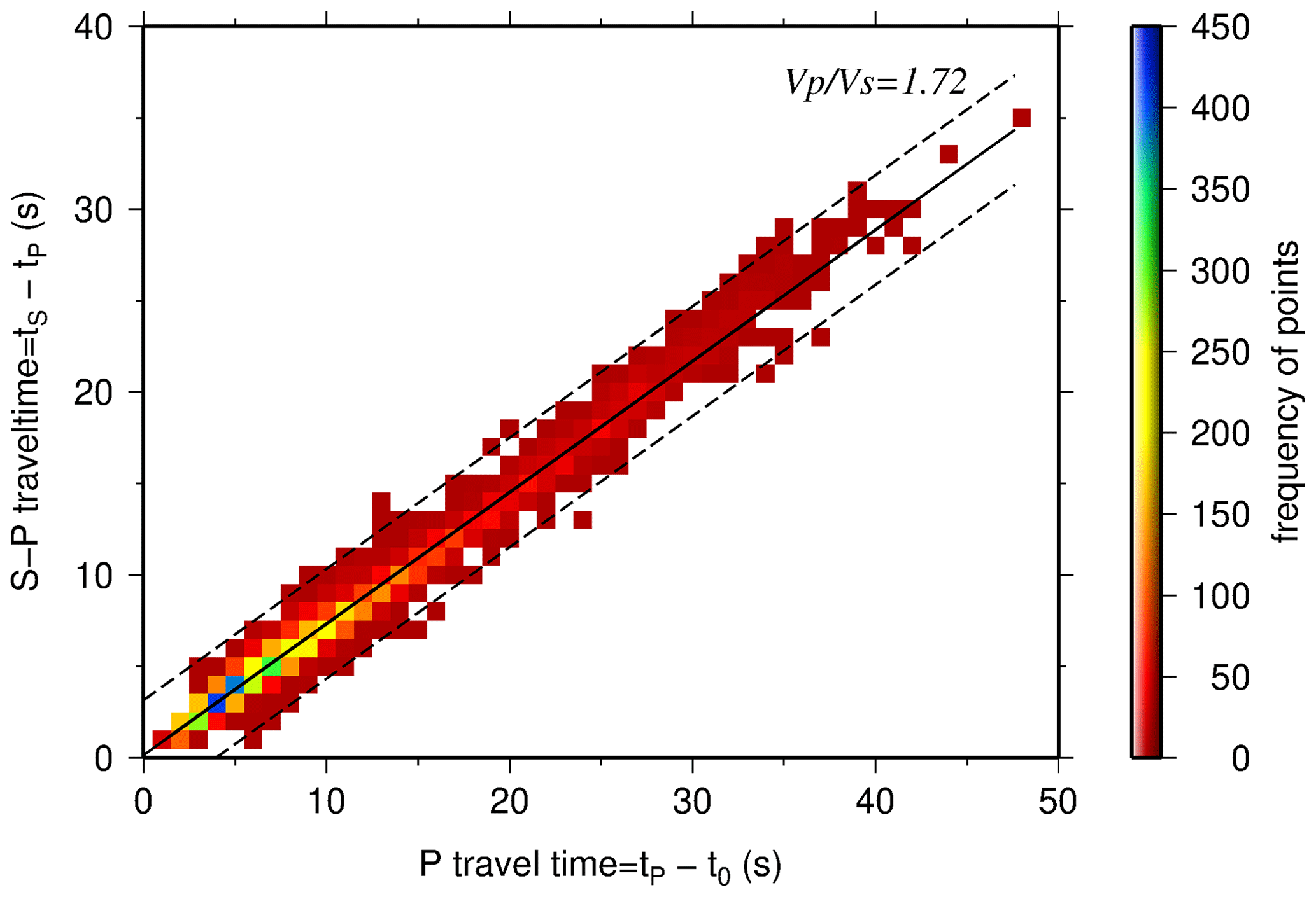
Figure 3Modified Wadati diagram based on P and S picks after visual (manual) analysis (the color indicates number of picks; please see the color palette table on the right). The origin times (t0) of the earthquakes are provided by the single-event localization using HYPO71 hypocenter determination program (Lee and Lahr, 1975). The solid black line shows the fit to the data by linear least squares, and its slope indicates the ratio of 1.72. The dashed lines show values with s.
For the simultaneous inversion of hypocenters, 1-D velocity models, and station corrections, we used the events with at least 10 P picks and 5 S picks and an azimuthal gap less than 180∘, which comprises 301 local earthquakes. The arrival time dataset consists of 11 084 P picks and 6496 S picks (quality classes of 0 to 3) with average picking errors of 0.12 and 0.21 s for P and S observations, respectively (Table 1). The average number of picks per event is 32 for P and 18 for S, with maximum of 157 and 118, respectively (Fig. 4).
Table 1Statistical parameters of high-quality P and S pick dataset of 301 well-constrained local earthquakes used for simultaneous inversion of hypocenters, 1-D velocity model, and station corrections.
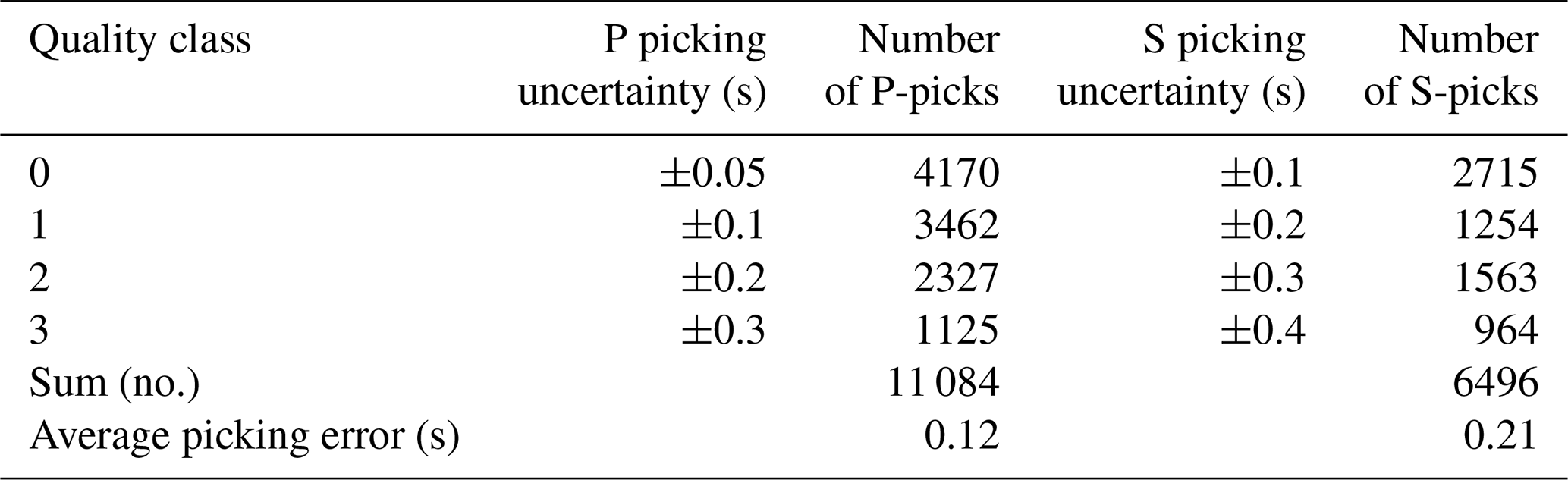

Figure 4Histograms of high-quality P and S picks per event for 301 well-constrained local earthquakes used for simultaneous inversion of hypocenters, 1-D velocity models, and station corrections.
In order to investigate the seismicity pattern, we use the travel time data of an additional 43 local earthquakes with slightly fewer picks (minimum of eight P picks and two S picks) to the main dataset and relocate them using the VP, , station corrections, and noise levels from the simultaneous inversion (Sect. 6.3). This updated dataset contains 344 earthquakes, 12 420 P picks, and 7192 S picks.
4.1 Probabilistic Bayesian inversion
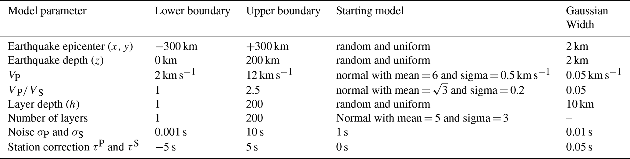
Considering that hypocenter locations and velocity model are inherently linked to each other (coupled hypocenter-velocity problem, e.g., Kissling, 1988; Thurber, 1992; Kissling et al., 1994), especially in the local earthquake case, a simultaneous inversion for hypocenters and velocity structure (and/or station corrections) is needed. In this study, different to the conventional approach of damped least squares, we use a Bayesian approach (Bayes, 1763). Bayesian approaches have been applied in a number of geophysical studies (Tarantola et al., 1982; Duijndam, 1988a, b; Mosegaard and Tarantola, 1995; Gallagher et al., 2009; Bodin et al., 2012a, b; Ryberg and Haberland, 2018). Ryberg and Haberland (2019) recently implemented a hierarchical, transdimensional Markov chain Monte Carlo (McMC) approach for the joint inversion of hypocenters, 1-D velocity structure, and station corrections for the local earthquake case. While with classical inversion techniques a discrete best-fitting model m (i.e., locations, velocity model, etc.) is derived, in the Bayesian inference all the parameters of the model m are represented probabilistically. For the theoretical background the reader is referred to Bodin and Sambridge (2009) and Bodin et al. (2012a, b). We define a uniform and wide range of values for each individual model parameter (before knowing the observed data; prior) and after performing the inversion for random combinations of the parameters, we derive a probability distribution individually for each model parameter (after combining the prior information with the observed data; posterior). Thus, a large suite of models is generated, all of them fitting the travel time observations. The choice of a uniform and extensively wide range of model parameters (Table 2) guarantees that the final model is dominated by the data rather than by the prior information (i.e., starting model, choice of parameters).
Table 2Prior distribution (model space), starting model, and width of Gaussian distribution for each model parameter.
4.2 Model parametrization and forward problem
Hypocenters are described by spatial (x0,y0,z0) and temporal (t0) coordinates and the 1-D velocity structure is described by a variable number of horizontal layers with individual values of VP and . Moreover, the model m comprises station corrections for P and S waves (τP and τS), which account for travel time effects (delayed or earlier arrivals) due to deviations of the 1-D model from the real 3-D velocity structure in the shallow subsurface beneath the stations. The inversion also derives the quality of the data expressed as noise levels for P and S picks (σP and σS), which are also unknowns in the inversion. The noise includes actual picking errors, systematic errors of observations or measurements, and any approximation or errors of forward travel time calculation (see below) and is assumed to be normally distributed and uncorrelated. Therefore, the complete model to be inverted for is defined as follows:
where K is the number of layers; h is layer depth; and i, j, and k refer to layer, earthquake, and station index, respectively. It should be noted that the number of layers is also unknown. In other words, the model space dimension is not fixed in advance and hence the posterior is a transdimensional function.
In order to sample models from the prior probability distribution, we apply McMC approach to create a huge number of different models m by random selection of model parameters (see Eq. 1 and Sect. 4.3). Accordingly, to compute travel times the forward problem has to be solved a very large number of times. We use the 2-D finite differences (FD) Eikonal solver (Podvin and Lecomte, 1991) for the forward calculation. This algorithm requires a regular mesh. Therefore, the irregular velocity model is converted to a fine and uniform mesh by setting the velocity at each mesh point to the value of the nearest point from the irregular model (VPi or i). The fine mesh used by the Eikonal solver has a cell spacing of 1 km vertically and horizontally.
Once the travel times are calculated, a misfit function, particularly for each model, is defined as the summed squared differences between the observed (d) and calculated travel times. The misfit function is then used to build the Gaussian likelihood function and the posterior values of the proposed model (for detailed information one could refer to Ryberg and Haberland, 2019).
4.3 Markov chain Monte Carlo (McMC) algorithm
Given the Bayesian approach described above, the McMC algorithm generates an ensemble of models with parameters within the prior distribution. We mainly follow the hierarchical, transdimensional procedure proposed by Ryberg and Haberland (2018, 2019) that supports the calculation of both model parameters and model dimensionality. The evolution of a model along the Markov chain consists of four main steps: (1) choose a random initial model m (Table 2). (2) Generate a new model from the prior distribution by perturbing the current model parameters (changing one of the velocity parameters of a random node, shifting the position of a random earthquake, adding a new layer, removing a random layer, altering one of the noise parameters, changing a randomly selected station correction. The changes in the VP, , cell position (i.e., layer), and noise levels must be according to Gaussian probability distribution centered at the current value. The values of the new model are randomly selected within very wide bounds (Table 2) and thus do not truncate the posterior probability distribution. (3) The forward calculation (Sect. 4.2) is then performed on the new model. The newly estimated travel time data are compared with the observed data d and then the misfit function, data likelihood, and the posterior probability are determined. (4) The newly proposed model is accepted or rejected based on the criteria of Bodin and Sambridge (2009). If the new model is rejected, then the current or old model is retained by reiterating step 2. However, there is still a probability of acceptance even if the fit of the new model is worse than that of the old model. If the model is accepted (i.e., when it is better than the previous model) then it acts as a starting model for another iteration (step 1).
By reiteration of steps 1 to 4, a chain of models is produced, which is in fact the Markov chain. This chain is continued until the misfit is no longer significantly decreasing (burn-in phase). Thereafter, a stationary model space sampling is achieved. If these sequences are repeated long enough, a chain provides an approximation of the posterior distribution for the model parameters. To accelerate the model space sampling, up to 1000 separate and independent chains are investigated in parallel.
The main idea of the McMC method is to keep prior assumptions of the model parameters (conventionally used as initial values) at a minimum and thus minimize unwanted artificial effects on the final model. Therefore, the McMC method only uses the travel times and does not directly depend on initial hypocenters, origin times, velocity models, or even the model parametrization (e.g., grid node spacing). Nevertheless, the selection of picks in the (semi-automatic) picking procedure involves the comparison of the observed travel times with those based on preliminary hypocenters (which depend on initial velocity models). Therefore, the results of the inversion can sensu stricto depend to some degree on initial values.
As a variable Moho topography and complex lithosphere structure are expected for our study region, the 1-D model derived by and used in our inversion can only be a rough abstraction of the real conditions. Nevertheless, this simplification could potentially have influence on earthquake location correctness and accuracy. To assess the performance of our inversion strategy in this respect, using a 3-D velocity model and earthquake and station distribution of the real data, we calculated the synthetic travel times, added synthetic noise and finally inverted them in the same way as the real data (see below). Comparing input event locations (synthetic) and the inverted (output) ones allows us to study the recovery of the hypocenters, location consistency, and potential systematic errors related to the use of a 1-D model, which we can generally expect for the derived real hypocenters. For example, it can be studied whether events at the periphery or in certain parts of the model have systematically larger uncertainties (e.g., due to their location and/or spatial distribution of picks). Furthermore, we can study how the (output) 1-D model looks in comparison to the (input) 3-D model, how large the derived noise is in relation to the synthetic input noise, and how the pattern of station corrections corresponds to the shallow velocity anomalies. Similar tests are standard in structural studies (i.e., LET) to study the recovery of certain features.
In our synthetic 3-D background model, the course of the crust–mantle boundary is inspired by the Moho topography of the European and Adriatic plates from Spada et al. (2013); however, we adopted it in a simplified way without features such as crustal stacks (overlapping Mohos of the two involved plates) or the proposed Moho hole. Our main aim of this simplified adaption is studying the influence of a 1-D model class on the derived hypocenters after the inversion and the goal is not recovering the exact velocity structure. We assigned typical crustal velocities to the upper layer, starting with 6 km s−1 and increasing to 7 km s−1 at the base of this crustal layer. Thereafter, the velocity increases from 7 to 8 km s−1 within a thin zone of 3 km with a strong gradient. Following this, the velocity increases again gradually until it reaches 8.05 km s−1 at 90 km depth (Kennett et al., 1995; Christensen and Mooney, 1995). The Moho depth in the target area changes from 22 km along the flank of the Ivrea body to more than 55 km along the Adria–Europe plate boundary (Spada et al., 2013). We considered the model's surface to be −5 km to avoid wave propagation through the air.
In order to simulate realistic 3-D effects in the context of expected crustal structure, we superimposed shallow high- and low-velocity anomalies onto the background 3-D model presented above. We assumed that the hard rocks of the European basement exhumed in the TW have higher velocities than the surrounding Austroalpine nappes and thus form a high-velocity anomaly (+5 %) within a rough outline of the TW and from the surface to the depth of 10 km (for more information on the TW, see, e.g., Bertrand et al., 2015). Furthermore, we designed lower-velocity anomalies for the PoB and MoB sedimentary basins (the coarse outlines of the basins are taken from Waldhauser et al., 2002). An average VP of 4.35 km s−1 is considered for the entire MoB from the model's surface down to 2 km depth. For the PoB, a layer of 6 km thickness starting from the model's surface and with VP of 2 km s−1 less than the background model is constructed. The shallow anomalies are then inserted in the background model. Taking the shallow anomalies into account not only makes the model more realistic but also allows us to check whether the station corrections reflect travel time deviations due to velocity variations in the shallow subsurface. Figure 5 displays the 3-D synthetic VP model from different views and also the 1-D model at two different viewpoints. The ratio in the entire model is set to .
The P and S arrival times are calculated using the 3-D FD Eikonal solver (Podvin and Lecomte, 1991; Tryggvason and Bergman, 2006). We generated an FD grid with an increment of 1 km horizontally and vertically, resulting in a grid dimension of 601 × 321 × 96 with a total number of 18 520 416 nodes. For simulating a realistic travel time dataset, we adopted the geometry of stations and hypocenters of the real data. Using 344 earthquakes, in total 12 534 P and 7258 S synthetic picks resulted from the forward calculation. Thereafter, according to the manual arrival time uncertainties in Table B2, we added random noise (0.05, 0.1, 0.2, 0.3, 0.1, 0.2, 0.3, and 0.4 for P-0, P-1, P-2, P-3, S-0, S-1, S-2, and S-3, respectively) to the arrival times, and this dataset was then used for the simultaneous inversion by McMC.

Figure 5The 3-D synthetic VP velocity model. The ratio was fixed to in the entire model. (a) and (b) Contours of the Moho and shallow anomalies of the PoB, MoB, and TW from different view directions. (c) Modified Moho depth map based on Spada et al. (2013). (d) A 1-D velocity model of two different locations with shallower and deeper Moho retrieved from the 3-D synthetic velocity model (the locations are shown with red and black crosses in (a) and (c), respectively). The faults are the same as those in Fig. 2.
To explore the model parameters, 100 Markov chains each with 1000 random initial models are used for simultaneous inversion of McMC. Following the strategy in Ryberg and Haberland (2019), we derived ∼ 15 000 of the final models from the Markov chains (more information is given in Sect. 6) to define model parameters based on the average μ and standard deviation σ. For the earthquake epicenters (x and y) and station corrections (τP and τS) the classical average of the Gaussian distribution is used. However, the depth distribution of shallow earthquakes is truncated by the upper model boundary. In order to accommodate this, we used an algorithm based on truncated Gaussian distributions (Ryberg and Haberland, 2019) to derive true depth averages and uncertainties. The VP and values are defined based on the modified average (Ryberg and Haberland, 2018) and standard deviation.
Figure 6 represents the recovery of the earthquakes. Figure 6a shows that the epicenters are recovered very well (the blue dots are located on top of red circles). Further assessment of the earthquake recovery (Fig. 6b) demonstrates that the average misfit between synthetic and recovered hypocenters is quite close to zero with uncertainties of ∼ 400 m in epicenter, 1.31 km in depth, and 0.12 s in origin time. Nevertheless, we note that although the epicenters of most of the earthquakes throughout the study area are recovered well, the depths of the events at the edges of the network are less well recovered and that their uncertainties are also systematically larger (see Fig. 6). The recovered noise levels, which are representative of the unresolved part of the travel times, are calculated for individual pick types and quality classes separately (Fig. 6c). They are close to the random noise, which was added to the synthetic arrival times (manual arrival time uncertainties in Table B2); however, they are slightly higher. This deviation could be explained by the forward modeling errors and the fact that the inversion derives a 1-D velocity model from data of a 3-D input model.

Figure 6(a) Recovery of the hypocenters after synthetic test. Red circles are recovered earthquakes with a 1σ error bar (error bars of latitude and longitude are invisible at this scale), and blue dots are the synthetic locations. The gray triangles show the stations. (b) Histograms of the misfit between recovered hypocenters and original ones. The hypocenters are recovered very well, with an average misfit of 20 m (±380 m) in longitude, 210 m (±400 m) in latitude, 110 m (±1.131 km) in depth, and 0.12 s (±0.08 s) in origin time. (c) The recovered noise levels after McMC for individual pick types and quality classes are slightly higher than the random noise, which was added to the synthetic travel time data.
Figure 7a shows the derived VP and models as heat maps (posterior distribution of all the models). In addition, it shows the average value (red line), standard deviation of all the inferred models (yellow zone), and a reference model with maximum likelihood (blue line), i.e., maximum posterior probability (similar to Ryberg and Haberland, 2019). As seen, no clear single Moho velocity jump is recovered, but it is modeled by a gradual increase of the velocities at depths from 30 to 50 km. We attribute this to the variable Moho topography, which cannot be modeled by the 1-D velocity model per se, and potentially lower resolution due to less ray coverage in this depth range. Because of a dense ray coverage from the surface down to a depth of ∼ 20 km, the VP uncertainty is almost zero in this depth range. In the depth interval with strong Moho topography, the uncertainty varies between 0.1 and 0.66 km s−1. The uncertainty values are compatible with the standard deviation of the lateral heterogeneity in the synthetic 3-D velocity model (∼ 0.8 km s−1 above 2 km, ∼ 0.05 km s−1 between 2 and 20 km, and between 0.1 and 0.5 km s−1 below 20 km depth). Thus, we think that the increased standard deviations beneath ∼ 30 km depth indicating reduced and fading resolution are due to both variable Moho topography and reduced ray coverage; however, their exact contribution is hard to discern.
The ratio was fixed to the square root of 3 for the whole region in the forward modeling, and the same value is recovered down to ∼ 35 km depth with almost zero uncertainty (less than 0.02). The uncertainty of increases below 35 km depth to a maximum value of 0.046, indicating that this deeper part of the model is not well resolved.
The station corrections (Fig. 7b) correspond to a large extent to the shallow anomalies of the 3-D synthetic model (Fig. 5). The shallow high-velocity anomaly in the TW is expressed by negative corrections (large circles) corresponding to earlier arrivals, while the shallow low-velocity anomalies of the PoB and MoB correspond to positive corrections (large crosses) reflecting later arrivals.

Figure 7(a) Recovery of the VP and models after the synthetic test. The results are shown with heat maps (probability histogram vs. depth; warm and cold colors correspond to higher and lower probabilities, respectively) with gray areas showing zones with no model achievement. The modified average model (solid red line), most probable model (solid blue line), and corresponding uncertainty of 1σ (yellow zone) for both VP and models are shown as well. The ratio of is displayed with the dashed green line. (b) Recovered P wave station corrections of all the stations that were involved in the McMC inversion. Blue crosses show positive values reflecting lower velocities, and red circles display negative values indicating higher velocities than expected. Regions indicated in gray have shallow high- or low-velocity anomalies (see Fig. 5 for more information). Symbol size corresponds to correction amplitude. The faults are same as Fig. 2.
For the simultaneous inversion of the hypocenters, the 1-D velocity model, and the station corrections, we used the travel time dataset of the earthquakes (Sect. 3.2). In the simultaneous inversion, for the first 300 000 models of the Markov chains, only the hypocenters are allowed to be changed. Thereafter, VP, ratio, station corrections, and noise levels additionally are permitted to change, adding 300 000 more models to the Markov chain. After inversion of 400 000 models in each Markov chain, the model space reached the stationarity (end of burn-in) phase. Thereafter, badly converging chains are automatically excluded, and every 1000th model is stored from the remaining models after the burn-in phase. The stored models of each chain are combined (in total ∼ 15 000 models) to calculate the posterior probability. The final models have stationary rms misfits of 0.36 s (Fig. 8).
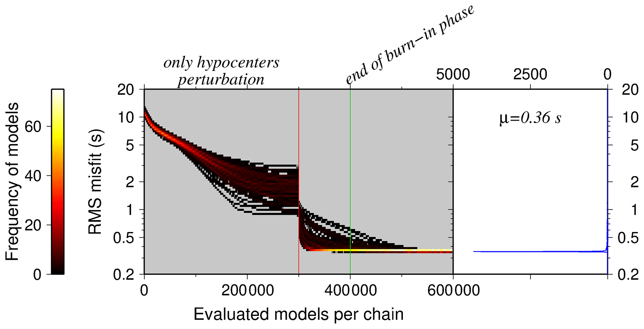
Figure 8On the left histogram, the rms misfit along Markov chains during the inversion evolution is shown (color indicates number of models; please see color palette table on the left). Before the red line (300 000 models), only the hypocenters are perturbed and beyond that the VP, ratio, station corrections, and noise levels are allowed to change as well. The green line indicates the end of the burn-in phase after ∼ 400 000 models. On the right histogram, the rms misfit for all the models after burn-in phase is shown. The best-fitting models are characterized by an average 0.36 s rms misfit.
6.1 The 1-D velocity model and station corrections
It turns out that the algorithm needs roughly five layers to best fit the data (Fig. 9a). Similar to the synthetic test (Fig. 7), the final velocity models are shown with the average of all remaining models and the model with maximum posterior probability. In general, for both VP and models (Fig. 9b) the average value (red line) varies gently, whereas the model with maximum posterior probability (blue line) is rather coarse and contains discontinuities.
The derived VP model starts with a rather high value of 5.94 km s−1 at the surface and increases only very gently down to a depth of around 20 km. After a zone of higher velocity gradient in the average model around (and a step-like increase of the reference model at) ∼28 km depth, velocities reach ∼6.8 km s−1 at ca. 30 km (down to ca. 45 km depth). Down to this depth the uncertainties (1σ) indicating the resolution increase from 0.01 km s−1 (very good) to 0.28 km s−1 (fair). Our derived VP model in the upper crust – except for the uppermost layer shallower than 3 km – is similar to the Diehl et al. (2009b) model, an increase for values above 6.5 km s−1 is observed deeper than in the latter model.
Below ca. 45 km depth, velocities increase further up to 7.85 km s−1 at 60 km depth; however, standard deviations (1σ) between 0.3 and 0.42 km s−1 indicate only poor resolution in this depth range. A single step-like increase from “crustal” to “upper mantle” velocities (as at 35 km depth in the Diehl et al. (2009b) model) cannot be observed, which we attribute either to (1) the expected strong depth variability of the Moho in the study area (see the discussion of the synthetic model in Sect. 5) and a gradual course of the 1-D model due to lateral averaging in this depth range, (2) the relatively small number of Pn arrivals, and/or (3) limited maximum observation distances. Influences by wrongly picked late-arriving Pg arrivals at large distances (instead of Pn phase) cannot totally be ruled out.
As a 1-D model cannot be representative of the 3-D structure, especially in a region with expected irregular Moho and complex crustal structure, a geologically meaningful interpretation of the derived VP model is hardly possible.
The model starts with high values at the surface (to ∼ 5 km depth) and shows reduced values of around 1.70 down to 22 km depth before reaching 1.77 at greater depths (with uncertainty between 0 and 0.02). However, 1σ values of 0.02 to 0.045 indicate only poor resolution at depth larger than around 30 km, which we associate to only a few Sn arrivals. This was basically expected from the Wadati diagram (Fig. 3) and is in agreement with values previously derived, e.g., by Viganò et al. (2013). Both VP and models are available in the Supplement S1.
The station corrections derived from the McMC simultaneous inversion potentially indicate local, shallow 3-D velocity anomalies in the subsurface, which cannot be accounted for by the 1-D model. The McMC inversion assumes that P and S station corrections have an average of zero. Negative corrections indicate earlier wave arrival and thus higher velocities in the (shallow) subsurface, whereas positive correction implies delayed arrival that is indicative of lower velocities.
The pattern of corrections (Fig. 9c) shows coherent negative corrections associated with the EA, ESA, and CA. The large negative values in the eastern part (east of 15∘ E) might be related to proximity to the edge of the network and thus be dominated by mantle phases (faster arrivals). Surprisingly, in between the negative values in the Alpine Chain, a pattern of slight positive corrections in the WSA is observed. Besides, extreme positive corrections are seen in the PoB and MoB as expected for sedimentary basins, which is also consistent with the results of the synthetic test (see Sect. 5). A pronounced pattern specifically related to the TW as seen in our synthetic test is not observed so clearly in the real data, suggesting a different structure in the shallow subsurface. The pattern of stations in the ESA and a few stations in the WSA and CA agree very well with results by Diehl et al. (2009b).
A detailed interpretation of the pattern of the station corrections is highly ambiguous because they contain a superposition of site effects and/or effects from 3-D structural variations, as well as a lot of smearing. Nevertheless, the general concept of simultaneously inverting local earthquake datasets for a (simplified) 1-D velocity model, hypocenter positions, and origin times and reactions proved to be very powerful for accurately localizing earthquakes (see e.g., Kissling, 1988). Moreover, the general pattern of corrections can indicate the consistency of phase data.

Figure 9(a) On the left histogram, the probability of the number of layers of the random models introduced by Markov chains during the evolution are shown (color indicates number of models). On the right histogram, the number of layers of the models after burn-in phase is given. (b) VP, , and VS models after McMC simultaneous inversion. Figure characteristics are similar to Fig. 7. The velocity models are recovered down to ∼ 63 km depth. (c) P wave station corrections of all the stations that were involved in the inversion corresponding to the 1-D velocity model in (b). Negative corrections (red circles) indicate earlier arrivals (indicative for higher velocities in the shallow subsurface) and positive corrections (blue crosses) indicate delayed arrivals (representative for lower velocities underneath the station). The faults are same as in Fig. 2. Abbreviations are as follows: CA stands for central Alps, EA stands for eastern Alps, ESA stands for eastern southern Alps, WSA stands for Western Southern Alps, MoB stands for Molasse Basin, and PoB stands for Po Basin.
6.2 Estimation of hypocenter accuracy based on relocation of quarry blasts
To validate the localization procedure, the detected 15 quarry blasts (based on visual inspections; see Sect. 3.2) were independently relocated by McMC using the previously derived 1-D velocity model and station corrections from the simultaneous inversion (Sect. 6.1). Figure 10 focuses on the blast distribution associated with two quarry areas close to the villages of Albiano (Italy) and Gummern (Villach, Austria). After the relocation of the blasts, we see that the epicenters are located within the quarry areas and that the depths are in the range of the quarry topography (considering the average uncertainty of 1σ), some of them are offset by a maximum of hundreds of meters. Based on the average mislocation of the blasts (relative to the centers of the quarry areas) and also their location uncertainties, we estimate the absolute location errors in the range of 1 km horizontally and 500 m vertically. This indicates that although the number of picks is generally lower for blasts, the McMC routine provides high-precision hypocentral solutions. It is expected that the errors of earthquakes (which are potentially deeper than blasts) are smaller than those estimated from this test because they are less affected by the heterogeneous shallow structure, which was poorly accounted for by the model (Kissling, 1988; Husen et al., 1999).
The hypocentral solutions of the blasts, in comparison with those obtained by INGV/ZAMG, have an average difference of ∼ 160 m in longitude, ∼ 1 km in latitude, and ∼ 4.6 km in depth, and thus the depths are considerably better resolved and recovered in our study due to the availability of the denser SWATH-D network.
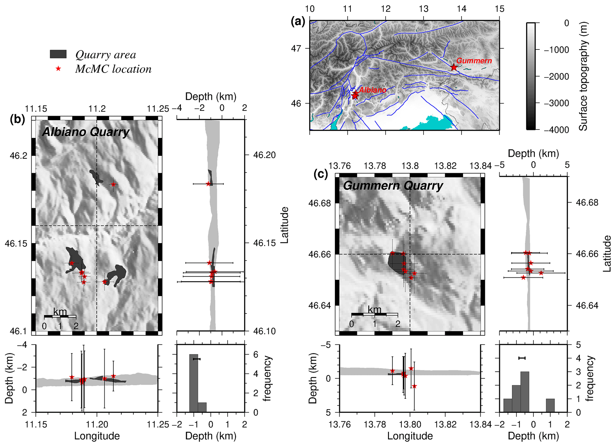
Figure 10(a) Map view showing the location of quarry blasts relocated using single-event mode of McMC, with solutions of the 1-D velocity model and station corrections from the simultaneous inversion of earthquakes. (b) and (c) Epicenter and depth distribution of the blasts associated with two quarries close to Albiano in Italy and Gummern in Austria, respectively. The light gray band in the cross sections shows the surface elevation variation within the map view boundary. The dark gray zones show the location and surface elevations of the quarries. The depth histogram is also shown for each quarry (the bar in the depth histograms displays the surface elevation within the quarry area). Please note that elevations above the sea level are shown with negative values.
6.3 Seismicity distribution
The distribution of seismicity in the southern and eastern Alps is shown in map view and cross sections in Figs. 11 and 12. This includes the same 301 events used for the simultaneous inversion (Sect. 6.1), as well as 43 additional earthquakes with slightly lower quality (see Sect. 3.2). For this relocation, we used the modified average VP and models, station corrections, and noise levels that resulted from the simultaneous McMC inversion. After relocation, the depth probability distribution of nine earthquakes was not Gaussian, and thus (due to their high depth uncertainty) we decided to remove these earthquakes from our catalog. Based on statistical analyses of the McMC inversion, the average epicentral and depth uncertainties (1σ) are ∼ 500 m and ∼ 1.7 km, which are compatible with precision estimates by the synthetic test (Sect. 5). However, the absolute location errors estimated by quarry blasts test (Sect. 6.2) are ∼ 1 km for epicenter and ∼ 500 km for depth.
Since the national agencies are (probably) using much less data for the location (smaller number of stations used, larger inter-station distances), a significant difference between their hypocenter solutions and those obtained in this study is expected (average of 2.4 km in epicenter and 3.7 km in depth). The earthquake depths calculated by McMC are systematically shallower than those by national agencies (by an average of 1.1 km). The maximum and minimum differences in the epicenters and depths (between McMC and national catalogs) are seen for the earthquakes from the INGV and SED, respectively.
The derived hypocenters in this study are not a representative seismicity catalog for the region (the national catalogs contain also many small, poorly constrained events in a much longer period) but form excellent data for further seismological studies, e.g., local earthquake tomography (LET). Moreover, these highly precise hypocentral data allow further tectonic inferences. The hypocenter solutions of constrained earthquakes derived in this study are available in the Supplement S2.
The seismicity is clustered in the same areas as in previous seismic studies of the region (e.g., Reiter et al., 2018). The long-term seismicity by, e.g., merged national catalogs and the SHARE catalog (Grünthal et al., 2013) also indicates the similar seismicity pattern. Most activity is seen within the orogenic retro-wedge in the FV region, with somewhat lesser activity in the SW part of the Giudicarie Belt (GL region). Further activity is located in the Austroalpine nappes north of the PAF and the region around Innsbruck (upper and lower Inntal and the Stubai Alps). The earthquakes reach a maximum depth of ∼ 20 km (Fig. 11), most of them occurring in the depth range of 5 to 15 km. Regions of little or no seismicity are observed at the northeastern corner of the eastern Adriatic or Dolomites indenter, southeast of the NGF (e.g., Reiter et al., 2018), and north of the PAF (Fig. 11).
The overall pattern of seismicity reflects the head-on convergence of the Adriatic indenter with the Alpine orogenic crust, accommodated along thrust faults and folds in the FV region and segmented in the western part of the ESA by strike-slip faults of the Giudicarie Belt.
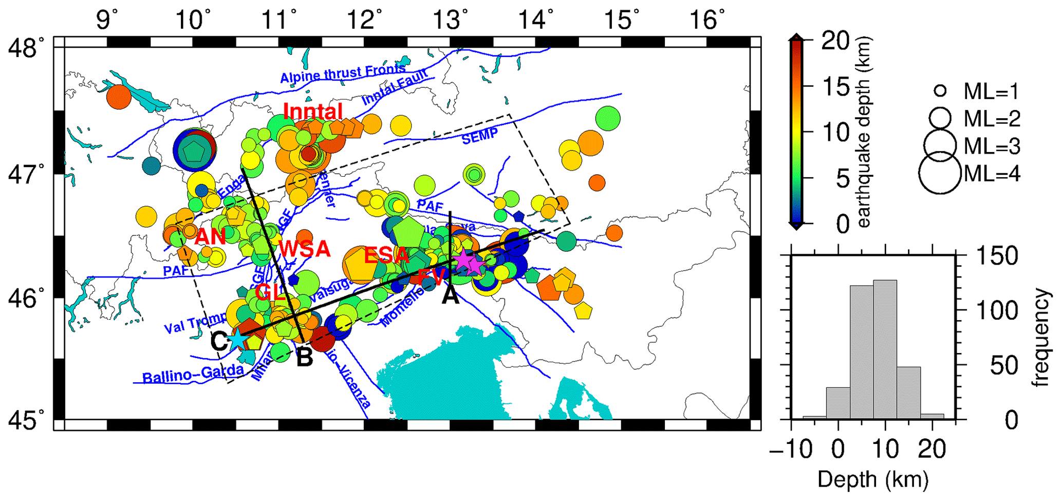
Figure 11Distribution of the 335 well-located earthquakes in the target area after McMC inversion (single-event mode). Circles are earthquakes that were incorporated in the simultaneous inversion, and pentagons are 43 additional earthquakes with fewer picks. The color and size of the circles indicate the depth and magnitude of the earthquakes, respectively (magnitude is taken from national catalogs). The dashed black box indicates the periphery of the SWATH-D network. Purple stars show the location of Friuli earthquake of 6 May 1976 (ML 6.4) and its major aftershock on 15 September 1976 (ML 6.1) (Slejko, 2018), and the blue star is the Salò earthquake on 24 November 2004 (ML 5.2; Viganò et al., 2015). Black lines indicate cross sections shown in Fig. 12. Faults are compiled from geological maps of the Italian geological survey, including Avanzini et al. (2010); Bartolomei et al. (1967); Bosellini et al. (1967); Braga et al. (1971); Castellarin et al. (1968, 2005); and Dal Piaz et al. (2007) and complemented by fault traces published in Handy et al. (2010) and Schmid et al. (2004, 2008). Abbreviations are as follows: ESA stands for eastern southern Alps, WSA stands for western southern Alps, FV stands for Friuli-Venetia region, GL stands for Giudicarie–Lessini region, AN stands for Austroalpine nappes, PAF stands for Periadriatic Fault, NGF stands for northern Giudicarie Fault, SGF stands for southern Giudicarie Fault. The histogram on the right side indicates the depth distribution of the earthquakes in the crust.
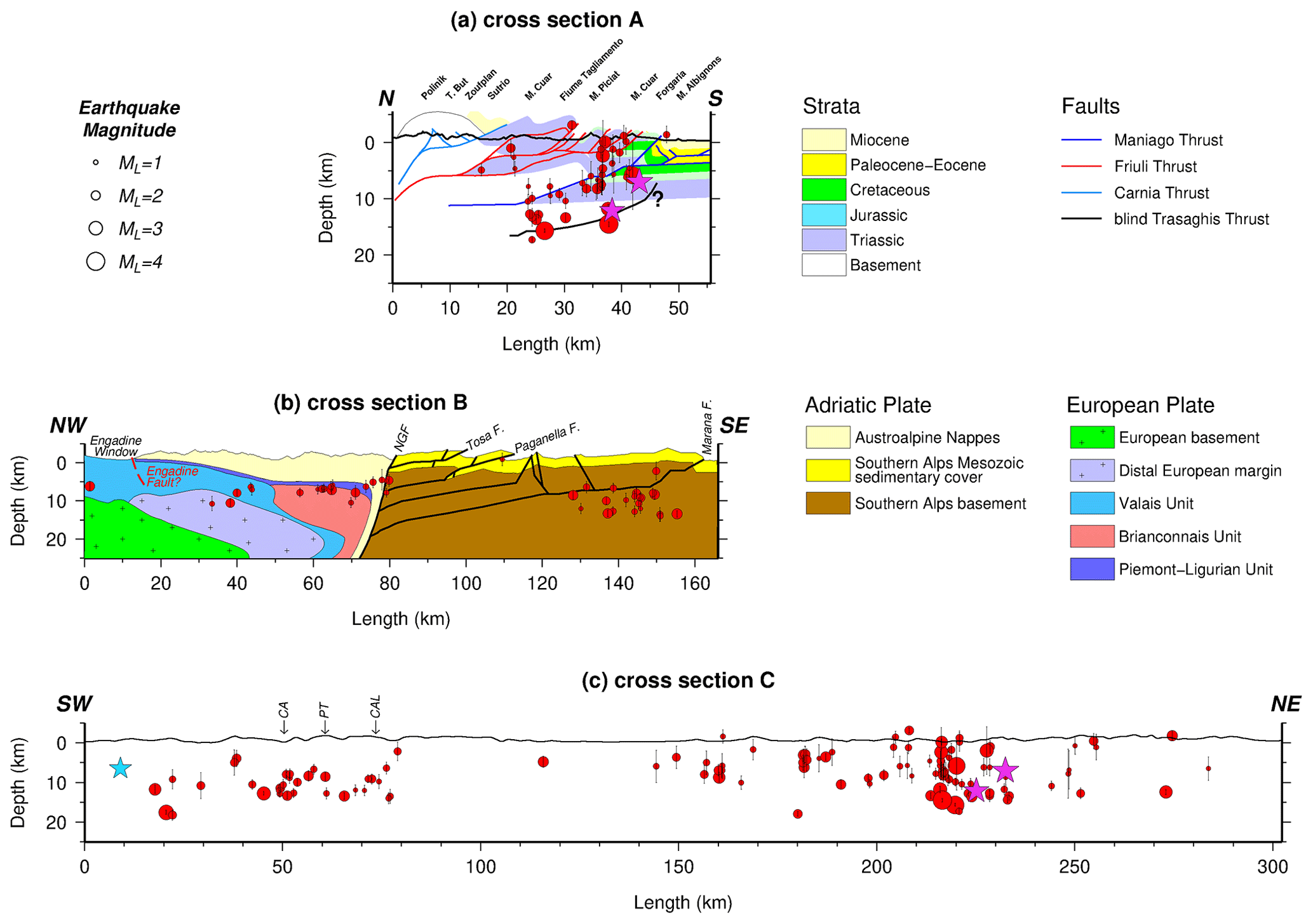
Figure 12Seismicity distribution in depth along three profiles of A, B, and C in Fig. 11. For better clarity, the depth and length scales of cross section A are magnified by a factor of 1.5 (without any distortion) compared to cross sections B and C. Red dots indicate hypocenters, projected from a swath extending to 15 km on either side of the profiles. Purple stars show the location of Friuli earthquake of 6 May 1976 (ML 6.4) and its major aftershock on 15 September 1976 (ML 6.1) (Slejko, 2018), and the blue star is the Salò earthquake on 24 November 2004 (ML 5.2; Viganò et al., 2015). Geological structures of the FV region along cross section A are modified following Nussbaum (2000) with the blind Trasaghis thrust taken from Galadini et al. (2005). Geological structures NW and SE of the NGF in cross section B are modified after Rosenberg and Kissling (2013) and Verwater et al. (2021), respectively. Abbreviations are as follows: NGF stands for North Giudicarie Fault, CA stands for Campofontana Fault, PT stands for Priabona–Trambileno Fault, and CAL stands for Calisio Fault.
6.3.1 Friuli-Venetia (FV) region
In accordance with the previous studies (and references therein Bressan et al., 2016; Reiter et al., 2018) and national catalogs, most of the seismicity in our dataset occurs in the ESA, i.e., within the FV region, coinciding with the eastern part of the deformation front between the Adriatic plate and the PAF. This was also the location of the destructive Friuli earthquake of 6 May 1976 (ML 6.4) and its major aftershock on 15 September 1976 (ML 6.1) (purple stars in Figs. 11 and 12a and c), which are associated with the Susans–Tricesimo Fault and buried or “blind” Trasaghis thrust, respectively (Poli et al., 2002; Galadini et al., 2005; Slejko, 2018). We find most earthquakes around 13∘ E (close to the villages of Tolmezzo and Gemona) down to a depth of around 17 km (Fig. 12a and c – around km 220, corresponding to 13∘ E). However, the seismicity is distributed over a wider area (see also Fig. 12c eastern part; between km 140 and 280). As stated above, a direct connection of individual earthquakes in our dataset to known faults near the surface is difficult. Nevertheless, the clustering of seismicity in the FV region between the Alpine frontal thrusts and the Fella–Sava fault in the north suggest that several frontal thrusts and backthrusts are active. Moreover, Petersen et al. (2021) shows a dominant E–W striking thrust mechanism for this region.
According to the fault distribution (and naming) of Galadini et al. (2005), the seismicity along the cross section A (Fig. 12a) indicates that the Susans–Tricesimo and Trasaghis faults (and potentially the Maniago thrust) are the most active faults in this region. Most earthquakes are located below the Maniago thrust, one of the main Alpine frontal thrusts in the tectonic model of Nussbaum (2000). This suggests that there is an active fault at greater depth (Fig. 12a). We interpret this to indicate a blind (i.e., that has not reached the surface) southward-propagating thrust front. In the profiles of Galadini et al. (2005) and Merlini et al. (2002) further east, this deeper blind thrust (named Trasaghis thrust in Galadini et al., 2005) reaches the surface, where it offsets Plio–Pleistocene sediments. More near-surface activity down to a depth of 6 km can generally be related to the Friuli thrust system (see Nussbaum, 2000, and Fig. 12a).
6.3.2 Giudicarie-Lessini (GL) region
The seismicity in the GL region correlates with the NNE–SSW transpressive fault system of Giudicarie Belt and the NW–SE-trending Schio–Vicenza strike-slip fault system. Seismicity of the Giudicarie fault system is concentrated mainly in the south (southwest of Lake Garda at depths ranging from a few kilometers down to 15 km; Fig. 11) and is in agreement with Viganò et al. (2015). For this part of the Giudicarie Belt, Viganò et al. (2008) suggested the kinematic regime of thrust with a strike-slip component (see also Petersen et al., 2021). The big Salò earthquake on 24 November 2004 with ML=5.2 and a thrust mechanism (blue star in Figs. 11 and 12c; Viganò et al., 2015) was suggested to have occurred on a low-angle thrust connected to the steep Ballino–Garda Fault, which detaches the sedimentary cover (hanging wall) from the underlying crystalline basement in its footwall (Viganò et al., 2008, 2013, 2015).
The NNW–SSE trending system of vertical strike-slip faults making up the Schio–Vicenza Fault is located between the active NW-dipping thrusts of the Giudicarie Belt to the west and the NNW-dipping thrusts of the Valsugana thrust system to the east. The short observational period of our network and the low seismicity rate limits the unambiguous association of the earthquakes to specific faults. However, some of the captured seismicity seems to take place along the Campofontana (CA), Priabona–Trambileno (PT), and Calisio (CAL) faults (Fig. 12c – western section). The Schio–Vicenza fault system is the most active structure in the GL region and was shown with predominant right-lateral strike-slip mechanism (Viganò et al., 2008).
Figure 12b shows the distribution of seismicity superposed on the main geological structures, which indicates that seismicity is focused in its southern part of the GL region. This suggests that the most southern and deepest faults (Fig. 12b) remain active, while the more internal fault systems have become seismically inactive (Verwater et al., 2021). Moreover, we observe that the seismicity is deeper than the frontal thrust modeled from balanced geological cross sections (Fig. 12b; Verwater et al., 2021), similar to observations within the FV region (as mentioned above). We interpret this to reflect southward propagation of the southern Alpine deformation front (blind thrusts) towards the Po Plain.
6.3.3 Lateral variations in clustering of seismicity from the WSA to ESA
A cross section running orogen-parallel from the GL to the FV region (Fig. 12c) indicates a similar depth of earthquakes for both regions. The FV region shows relatively high seismic activity, located at the junction with the Dinaric Front (Doglioni and Bosellini, 1987). However, in the central part of cross section C (around km 150 in Fig. 12c), sparse seismicity may indicate a seismic gap (Anselmi et al., 2011; Burrato et al., 2008). Alternatively, the sparse seismicity (especially at shallow depths) could indicate that deformation within this area is occurring aseismically, as proposed by Barba et al. (2013) and Romano et al. (2019) for the Montello thrust (Fig. 11). Strain rates within the Montello region are among the highest within the ESA (Serpelloni et al., 2016), which combined with its sparse seismicity indicates that the majority of deformation within this area is most likely occurring aseismically (Barba et al., 2013).
6.3.4 Engadine and Austroalpine nappes
The seismicity in the Austroalpine nappes (close to Italy–Switzerland border, Fig. 11) reaches a rather homogeneous depth around 11 km and does not seem to coincide with known geological structures in the area (e.g., Engadine Fault, Fig. 12b, left part). Although earthquakes are situated at a uniform depth, the distribution of these events in map view is quite diffuse (Fig. 11). Note that there are no seismicity clusters around the Engadine Fault in cross section B (Fig. 12b, left part), although the map view shows that seismicity coincides with the fault trace of the Engadine Fault NE and SW of cross section B. This could be related to block rotation along the Engadine Line (Schmid and Froitzheim, 1993).
6.3.5 Inntal region
A cluster of seismicity is found in the Inntal region at a depth range of 5 to 18 km (Fig. 11). This region is known for earthquakes with strike-slip and oblique-slip mechanisms that have been attributed to the activity of the Inntal Fault (Reiter et al., 2018; Petersen et al., 2021) and the Alpine basal thrust (Reiter et al., 2003). Historical earthquakes (e.g., the earthquake of 17 July 1670 in Hall in Tyrol; Hammerl, 2017) were also reported. Current seismicity (Fig. 11) extends further south into the Brenner region, where it has been associated with activity of the Brenner normal fault (Reiter et al., 2005).
6.3.6 Other structures
Several earthquakes in a depth range of 5 to 14 km are clearly aligned along the PAF between 12 and 12.5∘ E, possibly indicating ongoing activity of this fault (see also Reiter et al., 2018). The ENE–WSW Valsugana fault system does not seem to be seismically active, similar to the conclusion that Viganò et al. (2015) reached based on his analysis in the time frame of 1994–2007.
In this study, a semi-automatized picking procedure was applied to the waveform data recorded by SWATH-D and selected AlpArray network stations of earthquakes listed in national seismic catalogs. During the visual inspection of the picks, several quarry blasts were identified and separated from the earthquakes. In order to establish a very high-quality, consistent earthquake catalog in the study region, the arrival time data of the most constrained events (in terms of azimuthal gap, rms, and number of picks) were inverted simultaneously for hypocenters, 1-D velocity models, and station corrections using a McMC approach. A synthetic recovery test, using a close-to-realistic 3-D velocity model, validated the reliability of the method for yielding highly precise hypocenters even in complex 3-D velocity conditions. A quarry blast test demonstrated that the blast hypocenters are located very close to the quarry areas with average horizontal and vertical mislocations (relative to the centers of the quarry areas) of 740 and 376 m, respectively. The average uncertainties calculated by McMC for the earthquake locations are ∼ 500 m in epicenter and ∼ 1.7 km in depth. The derived VP and models are well resolved down to a depth of 30 km with an uncertainty below 0.45 km s−1 and 0.05, respectively. At greater depth the resolution decreases. Below 30 km depth, velocities gradually increase to mantle velocity, which is reached at around 50 km depth. The station corrections demonstrate coherent negative values associated with the EA, ESA, and CA and slight positive values in the WSA. Moreover, the PoB and MoB represent extreme positive corrections, as is expected for sedimentary basins.
The study is based on a very dense and large station network; however, it is limited to 16 months. Nevertheless, our precise hypocenter solutions with high internal consistency allow us to have insight into the active tectonic situation throughout the study region. The seismicity pattern confirms previous seismotectonic studies based on long-term records or local networks. Seismicity is found in diffuse clusters in the upper crust (0–20 km) and within broader zones of the Alpine frontal thrust, e.g., the FV region, along the GL and Schio-Vicenza domains, and in the internal Alpine and Inntal areas. The northeastern corner of the Adriatic or Dolomites indenter is obviously inactive or low active. We think that the overall pattern of seismicity reflects the head-on convergence of the Adriatic indenter with the Alpine orogenic crust, accommodated in the FV region and along the Giudicarie Belt. The seismicity in the FV and GL regions shows activities deeper than the modeled frontal thrusts, which we interpret as an indication for southward propagation of the Southern Alpine deformation front (blind thrusts). The seismicity in FV and GL indicates similar earthquake depths for both regions, while the sparse seismicity between them may indicate that the deformation within this area is most likely occurring aseismically.
The 1-D VP and models and the reassessed precise hypocenters will be utilized for investigating 3-D seismic velocities in the region using LET. The earthquake database is provided in Supplement S1 and S2.
The process of integrating events from the national seismological agencies is summarized in Fig. A1. It starts with getting events between September 2017 and the end of 2018 and confined to our study area with ML ≥ 1 from catalogs of INGV, OGS, ZAMG, and SED. Thereafter, three individual event lists of A for Italy, Slovenia, and Croatia from INGV; B for Germany and Austria from ZAMG; and C for Switzerland from SED are selected. The lists will be subsequently updated by the other three catalogs (one at a time, as described in Fig. A1). Eventually, the three lists are merged into one list, which totals 2639 local events in the study region.
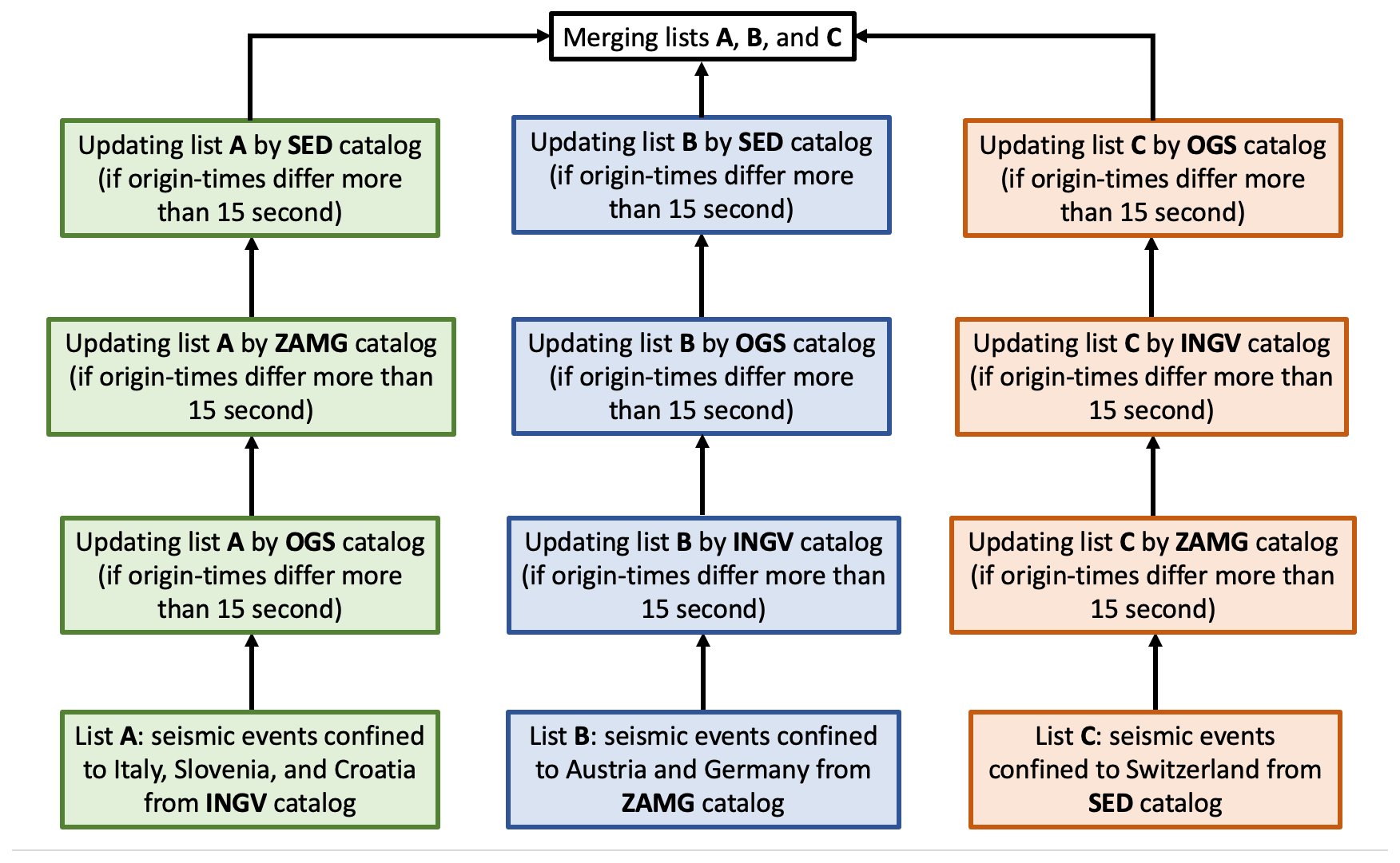
Figure A1Flow chart showing the process of merging seismic catalogs of INGV, OGS, ZAMG, and SED in order to derive an integrated seismic event list in the study region.
B1 Workflow
Our modified workflow consists of three main stages: (1) the NonLinLoc ray tracer (Lomax et al., 2000) for predicting initial P arrival times based on preliminary origin time and hypocenters (integrated earthquake catalog from national agencies) and the minimum 1-D velocity model of Diehl (2008); (2) the MPX algorithm (Aldersons, 2004; DiStefano et al., 2006) for improving the first alerts of P picks and classifying them into four quality classes (0 to 3, Table B2) based on Fisher statistics (Diehl, 2008, Appendix D: Users guide for MPX picking system); and (3) the Spicker algorithm (Diehl et al., 2009a) for picking S onsets based on P picks, event location, and a preliminary S pick (determined by NonLinLoc ray-tracing; Lomax et al., 2000). Spicker also rates picks into four quality classes (Table B2).
After each stage, in order to remove the effect of low-quality picks on hypocenter locations, a multiple relocation procedure using HYPO71 (Lee and Lahr, 1975) and various subsets of picks is performed. The procedure starts with localization of the events using the most reliable picks (higher-quality classes and closer distance to the event), and this first location is considered to be the reference for testing further picks. Thereafter, the picks with lower quality and those from distant stations are incorporated one-by-one. The newly added pick is kept if its residual is less than a distance-dependent, user-defined value and also if the root mean square (rms) residual of the event location is still acceptable (less than 1 s). Picks leading to unacceptable rms residuals are removed from the dataset. Moreover, in this relocation procedure, not only low-quality picks but also events with a small number of high-quality picks are removed. This procedure results in the location not being dominated by low-quality picks or not having sorted out better picks. Since MPX and Spicker depend on the correctness of the predicted arrival times (the predicted arrival time itself depends on the event location), picks and location are highly inter-dependent. This can be controlled by iteratively improving the event location, re-picking arrival times based on the updated location, and adding or removing dubious picks in each step.
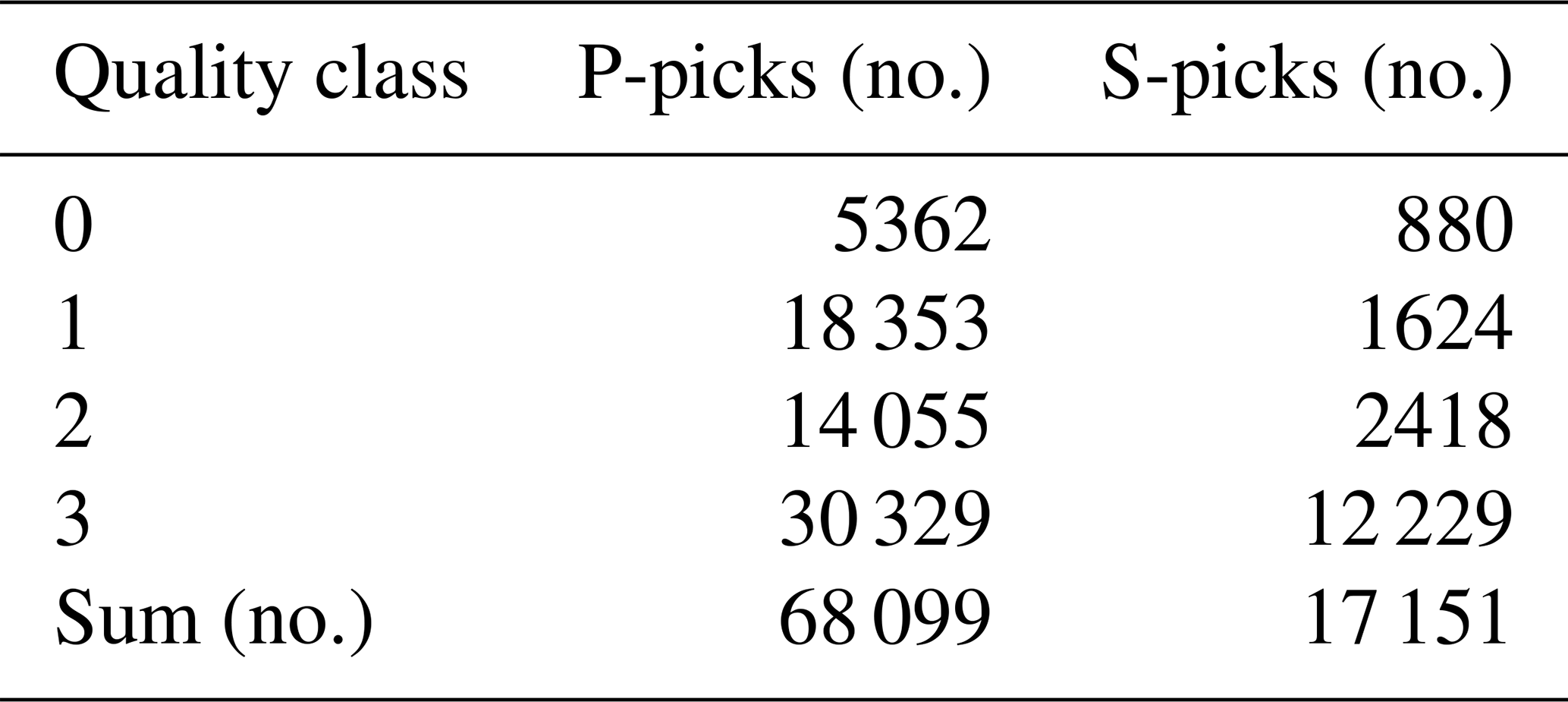
The implementation of this automatic workflow for the event list by national catalogs (Appendix A) resulted in a dataset with 2639 events, 68 099 P picks, and 17 151 S picks. The statistics of the picking quality classes are given in Table B1.
Table B1Distribution of the picks and their quality classes after implementation of the automatic picking algorithms for the event list created by national catalogs.
B2 Uncertainty assessment of arrival time picks
To assess the performance of the picking algorithms, a dataset consisting of 14 earthquakes with various magnitude ranges that are randomly scattered in the region are manually analyzed. Based on the arrival time uncertainty, the P and S picks are qualified into five classes (0, 1 ,2, 3, and 4, meaning 100 %, 75 %, 50 %, 25 %, and 0 % contribution into each location, respectively), and they are considered as reference for calibration (Table B2).
Table B2Statistics of the automatic and reference picks associated with the quality classes for a dataset of 14 earthquakes.
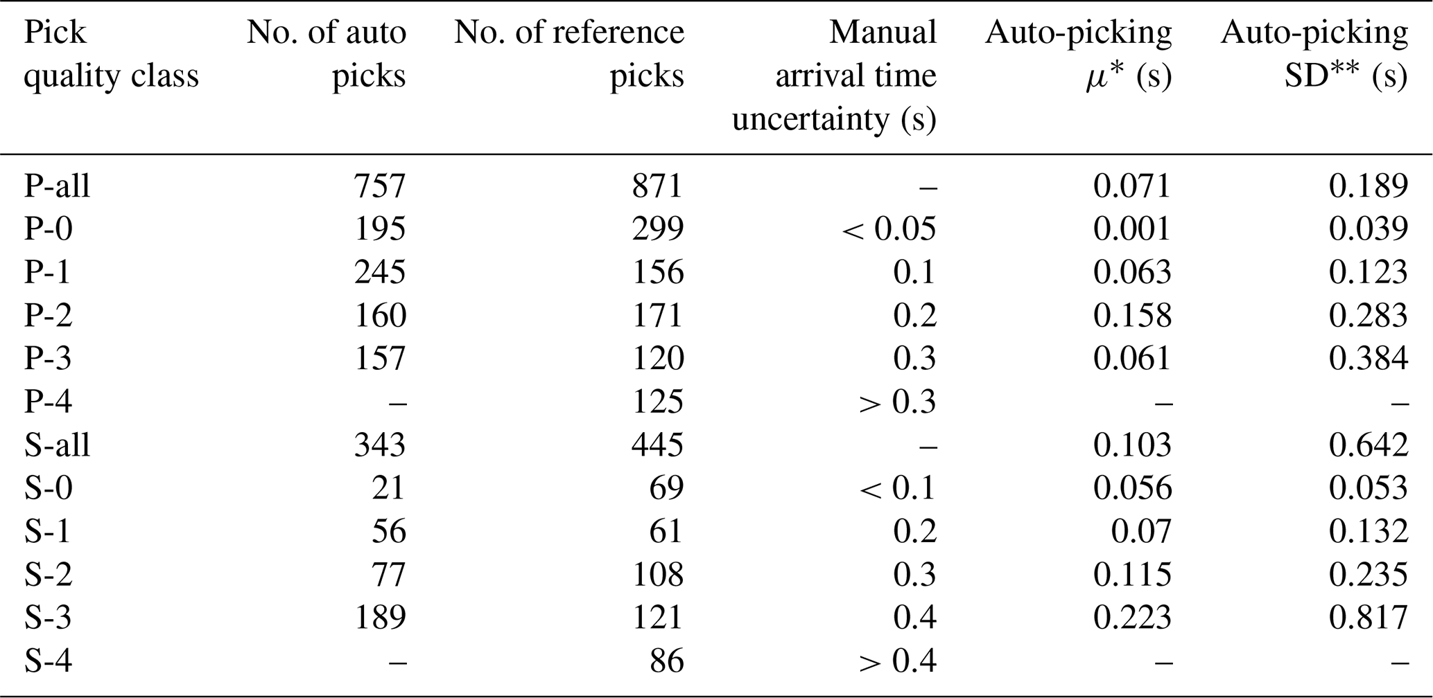
* The mean of misfits between automatic and reference picks.
** The standard deviation of misfits between automatic and reference picks.
The misfits between reference and automatic arrival times are calculated (individually for each quality class of the P and S picks) and the mean and standard deviation values are shown in Table B2. The picks with higher qualities have smaller mean values, which means their misfits are lower (i.e., automatic picks are closer to reference picks). Moreover, except for S-3, the standard deviation of each class is very comparable with manual arrival time uncertainty.
Another way of assessing the performance of the automatic picking algorithms is the so-called confusion matrix. The confusion matrix, in general, shows the performance of predicted vs. the actual data of different classifications in machine learning (Kohavi and Provost, 1998). For our dataset, it shows automatic picks vs. reference picks (similar to DiStefano et al., 2006; Diehl et al., 2009a; Sippl et al., 2013). In the confusion matrices displayed in Table B3, three values represent the performance of the automatic pickers in each quality class: (1) number of picks, (2) hit rate (fraction of reference picks of a certain class that are assigned to a specific class by the automatic picking) that is summed up to 100 % in each row, and (3) the standard deviation of the residuals between automatic and reference picks. The red and orange colors refer to picks that are upgraded to higher qualities by the automatic algorithms (unfavorable), whereas the green sectors show the picks that are underestimated by the automatic picker (more eligible). Having low hit rates in the orange and red cells and high hit rates in the green fields point toward a conservative assessment of the picking algorithms. The white fields in the confusion matrices illustrate the picks that are ideally qualified based on the reference dataset.
Table B3Confusion matrices of P and S picks, comparing the automatic picks with reference picks. Columns are quality classes of the automatic P picks from MPX (a) and S picks from Spicker (b), and rows represent the pick weighting classes provided by the human analyst for reference data. The parameters in each cell of the matrices are explained in the text.

The confusion matrices of both MPX and Spicker show relatively high values of hit rate (alternatively N) in some orange and red cells that we interpret as mispicks. For instance, the MPX (Spicker) picked 157 P picks (166 S picks) that are either ignored or qualified as class 4 by a human analyst. As the human analyst adopted class 4 for far stations with unclear arrivals, far automatic picks are unreliable. On the other hand, it seems that Spicker ignored a large number of picks (high hit rates in the most right column of the Spicker matrix). This is eminent for picks with manual quality class 0 that are potentially associated with the closest stations based on human analysis.
The SWATH-D data are archived at the GEOFON datacenter (https://doi.org/10.14470/MF7562601148; FDSN network code ZS, 2017–2019; Heit et al., 2017). Detailed information for accessing the data of permanent and temporary networks of AASN (network codes: BW, CH, GR, IV, MN, NI, OE, OX, RF, SI, SL, ST, Z3) is available at EIDA data access portal (http://www.alparray.ethz.ch/en/seismic_network/backbone/data-access/, last access: 1 November 2020). The earthquake hypocenters, together with the VP and models established in this study, are utilized in the Supplement.
The supplement related to this article is available online at: https://doi.org/10.5194/se-12-1087-2021-supplement.
The AlpArray Seismic Network Team: György Hetényi, Rafael Abreu, Ivo Allegretti, Maria-Theresia Apoloner, Coralie Aubert, Simon Besançon, Maxime Bes De Berc, Götz Bokelmann, Didier Brunel, Marco Capello, Martina Carman, Adriano Cavaliere, Jérôme Chéze, Claudio Chiarabba, John Clinton, Glenn Cougoulat, Wayne C. Crawford, Luigia Cristiano, Tibor Czifra, Ezio D’Alema, Stefania Danest, Romuald Daniel, Anke Dannowski, Iva Dasovic, Anne Deschamps, Jean-Xavier Dessa, Cécile Doubre, Sven Egdorf, Tomislav Fiket, Kasper Fischer, Florian Fuchs, Sigward Funke, Domenico Giardini, Aladino Govont, Zoltán Graczer, Gidera Gröschl, Stefan Heimers, Ben Heit, Davorka Herak, Marijan Herak, Johann Huber, Dejan Jaric, Petr Jedlicka, Yan Jia, Hélène Jund, Edi Kissling, Stefan Klingen, Bernhard Klotz, Petr Kolinsky, Heidrun Kopp, Michael Korn, Josef Kotek, Lothar Kühne, Krešo Kuk, Dietrich Lange, Jürgen Loos, Sara Lovati, Deny Malengros, Lucia Margheriti, Christophe Maron, Xavier Martin, Marco Massa, Francesco Mazzarini, Thomas Meier, Laurent Metral, Irene Molinari, Milena Moretti, Anna Nardi, Jurij Pahor, Anne Paul, Catherine Péquegnat, Daniel Petersen, Damiano Pesaresi, Davide Piccinini, Claudia Piromallo, Thomas Plenefisch, Jaroslava Plomerova, Silvia Pondrelli, Snježan Prevolnik, Roman Racine, Marc Régnier, Miriam Reiss, Joachim Ritter, Georg Rümpker, Simone Salimbeni, Marco Santulin, Werner Scherer, Sven Schippkus, Detlef Schulte-Kortnack, Vesna Sipka, Stefano Solarino, Daniele Spallarossa, Kathrin Spieker, Josip Stipcevic, Angelo Strollo, Bálint Süle, Gyöngyvér Szanyi, Eszter Szics, Christine Thomas, Martin Thorwart, Frederik Tilmann, Stefan Ueding, Massimiliano Vallocchia, Ludek Vecsey, René Voigt, Joachim Wassermann, Zoltán Wéber, Christian Weidle, Viktor Wesztergom, Gauthier Weyland, Stefan Wiemer, Felix Wolf, David Wolyniec, Thomas Zieke, Mladen Živcic, Helena Žlebcíková. The AlpArray SWATH-D Field Team: Luigia Cristiano (Freie Universität Berlin, Helmholtz Zentrum Potsdam Deutsches GeoForschungsZentrum – GFZ), Peter Pilz, Camilla Cattania, Francesco Maccaferri, Angelo Strollo, Günter Asch, Peter Wigger, James Mechie, Karl Otto, Patricia Ritter, Djamil Al-Halbouni, Alexandra Mauerberger, Ariane Siebert, Leonard Grabow, Susanne Hemmleb, Xiaohui Yuan, Thomas Zieke, Martin Haxter, Karl-Heinz Jaeckel, Christoph Sens-Schonfelder (GFZ), Michael Weber, Ludwig Kuhn, Florian Dorgerloh, Stefan Mauerberger, Jan Seidemann (Universität Potsdam), Frederik Tilmann, Rens Hofman (Freie Universität Berlin), Yan Jia, Nikolaus Horn, Helmut Hausmann, Stefan Weginger, Anton Vogelmann (Austria: Zentralanstalt für Meteorologie und Geodynamik – ZAMG), Claudio Carraro, Corrado Morelli (Südtirol/Bozen: Amt für Geologie und Baustoffprüfung), Günther Walcher, Martin Pernter, Markus Rauch (Civil Protection Bozen), Damiano Pesaresi, Giorgio Duri, Michele Bertoni, Paolo Fabris (Istituto Nazionale di Oceanografia e di Geofisica Sperimentale OGS – CRS Udine), Andrea Franceschini, Mauro Zambotto, Luca Froner, Marco Garbin (Ufficio Studi Sismici e Geotecnici – Trento) (also OGS).
AJN performed data preparation, analysis, and simultaneous inversion; she also prepared all figures and most of the text. CH supervised the analysis and contributed to the interpretation of the results. TR assisted with the inversion and modified the code. VFV, ELB, and MRH contributed to the interpretation and the discussion of results. MW promoted the work and performed text corrections. All co-authors contributed to the text and the figures.
The authors declare that they have no conflict of interest.
This article is part of the special issue “New insights into the tectonic evolution of the Alps and the adjacent orogens”. It is not associated with a conference.
We would like to express our appreciation to Ben Heit for the coordination of the SWATH-D network and to all people involved in the instrument preparation, field work, and data archiving (Team list above). We also give thanks to the numerous landowners for their willingness to host the stations and all communities, authorities, and institutes in the region for their great support of the project. Instruments for the SWATH-D network were provided by the Geophysical Instrument Pool Potsdam GIPP of the GFZ Potsdam. We also would like to acknowledge the AlpArray Seismic Network Team (Team list above). We thank the national seismological agencies of Italy (INGV, OGS), Austria (ZAMG), and Switzerland (SED) for their comprehensive earthquake catalogs. We also appreciate Christian Sippl for his guidance in implementing the automatic workflow. Discussions with many colleagues within the Priority program are greatly acknowledged. For plotting the figures, the Generic Mapping Tools (GMT; Wessel and Smith, 1991; Wessel et al., 2019) are used. The authors would like to thank reviewer Edi Kissling and the two other anonymous reviewers for their thorough and constructive remarks, which led to significant improvement of the manuscript.
This research and the seismic network have been supported by the German Science Foundation
DFG (grant nos. HA 3326/5-1, HA 3326/4-1, TI 316/6-1, and WE 1457/22-1) through the
special priority programme (SPP) “Mountain Building Processes in Four Dimensions (4D-MB)”.
The article processing charges for this open-access publication were covered by the Helmholtz Centre Potsdam – GFZ German Research Centre for Geosciences.
This paper was edited by Claudia Piromallo and reviewed by Edi Kissling and two anonymous referees.
Aldersons, F.: Toward a three-dimensional crustal structure of the Dead Sea region from local earthquake tomography, Ph.D. thesis, Tel-Aviv University, Israel, 2004. a, b
Amato, A., Barnaba, P. F., Finetti, I., Groppi, G., Martins, B., and Muzzin, A.: Geodynamic outline and seismicity of Friuli Venetia Julia region, B. Geofis. Teor. Appl., 18, 217–256, 1976. a
Anderson, H. and Jackson, J.: Active tectonics of the Adriatic Region, Geophys. J. Int., 91, 937–983, 1987. a
Anselmi, M., Govoni, A., De Gori, P., and Chiarabba, C.: Seismicity and velocity structures along the south-Alpine thrust front of the Venetian Alps (NE-Italy), Tectonophysics, 513, 37–48, 2011. a, b
Avanzini, M., Bargossi, G., Borsato, A., and Selli, L.: Note Illustrative della Carta Geologica d'Italia alla scala 1:50 000, foglio 060 “Trento”, APAT, Servizio Geologico d'Italia, 2010. a
Barba, S., Finocchio, D., Sikdar, E., and Burrato, P.: Modelling the interseismic deformation of a thrust system: seismogenic potential of the Southern Alps, Terra Nova, 25, 221–227, 2013. a, b
Bartolomei, G., Corsi, M., Dal Cin, R., D'Amico, C., Gatto, G., Nardin, M., Rossi, D., Sacerdotti, M., and Semenza, E.: Note illustrative della Carta Geologico d'Italia, foglio 21 “Trento”, Servizio Geologico d'Italia, 1967. a
Bayes, T.: An essay towards solving a problem in the doctrine of chances, Philos. T. R. Soc. Lond., 53, 370–418, https://doi.org/10.1098/rstl.1763.0053, 1763. a
Bertrand, A., Rosenberg, C., and Garcia, S.: Fault slip analysis and late exhumation of the Tauern Window, Eastern Alps, Tectonophysics, 649, 1–17, 2015. a
Bigi, G., Castellarin, A., Catalano, R., Coli, M., Cosentino, D., Dal Piaz, G., Lentini, F., Parotto, M., Patacca, E., Praturlon, A., Salvini, F., Sartori, R., Scandone, P., and Vai, G.: Synthetic structural-kinematic map of Italy, Sheets 1 and 2, C.N.R., Progetto Finalizzato Geodinamica, SELCA, Florence, Italy, 1989. a, b
Blundell, D. J., Freeman, R., and Mueller, S.: A continent revealed: The European Geotraverse, structure and dynamic evolution, Cambridge University Press, Cambridge, UK, 1992. a
Bodin, T. and Sambridge, M.: Seismic tomography with the reversible jump algorithm, Geophys. J. Int., 178, 1411–1436, 2009. a, b
Bodin, T., Sambridge, M., Gallagher, K., and Rawlinson, N.: Transdimensional inversion of receiver functions and surface wave dispersion, J. Geophys. Res.-Sol. Ea., 117, 1411–1436, https://doi.org/10.1029/2011JB008560, 2012a. a, b
Bodin, T., Sambridge, M., Rawlinson, N., and Arroucau, P.: Transdimensional tomography with unknown data noise, Geophys. J. Int., 189, 1536–1556, https://doi.org/10.1111/j.1365-246X.2012.05414.x, 2012b. a, b
Bosellini, A., Carraro, F., Corsi, M., De Vecchi, G., Gatto, G., Malaroda, R., Sturani, C., Ungaro, S., and Zanettin, B.: Note illustrative della Carta Geologico d'Italia, foglio 49 “Verona”, Servizio Geologico d'Italia, 1967. a
Braga, G., Gatto, G., Gatto, P., Gregnanin, A., Massari, F., Medizza, F., and Semenza, E.: Note illustrative della Carta Geologico d'Italia, foglio 22 “Feltre”, Servizio Geologico d'Italia, Rome, Italy, 1971. a
Bressan, G., Ponton, M., Rossi, G., and Urban, S.: Spatial organization of seismicity and fracture pattern in NE Italy and W Slovenia, J. Seismol., 20, 511–534, 2016. a, b, c
Burrato, P., Poli, M. E., Vannoli, P., Zanferrari, A., Basili, R., and Galadini, F.: Sources of Mw 5+ earthquakes in northeastern Italy and western Slovenia: an updated view based on geological and seismological evidence, Tectonophysics, 453, 157–176, 2008. a
Cagnetti, V. and Pasquale, V.: The earthquake sequence in Friuli, Italy, 1976, B. Seismol. Soc. Am., 69, 1797–1818, 1979. a
Castellarin, A., Corsi, M., De Vecchi, G., Gatto, G., Largaiolli, T., Mozzi, G., Piccoli, G., Sassi, F., Zanettin, B., and Zirpoli, G.: Note illustrative della Carta Geologico d'Italia alla scala 1:100 000, foglio 36 “Schio”, Servizio Geologico d'Italia, Rome, Italy, 1968. a
Castellarin, A., Picotti, V., Cantelli, L., Claps, M., Trombetta, L., Selli, L., and Carton, A.: Note illustrative della Carta Geologico d'Italia alla scala 1:50 000, foglio 080 “Riva Del Garda, Provincia Autonoma di Trento”, APAT, Servizio Geologico d'Italia, Florence, Italy, 2005. a
Cheloni, D., D'Agostino, N., and Selvaggi, G.: Interseismic coupling, seismic potential, and earthquake recurrence on the southern front of the Eastern Alps (NE Italy), J. Geophys. Res.-Sol. Ea., 119, 4448–4469, 2014. a, b
Christensen, N. I. and Mooney, W. D.: Seismic velocity structure and composition of the continental crust: A global view, J. Geophys. Res.-Sol. Ea., 100, 9761–9788, https://doi.org/10.1029/95JB00259, 1995. a
Dal Piaz, G., Castellarin, A., Martin, S., Selli, L., Carton, A., Pellegrini, G., Casolari, E., Daminato, F., Montresor, L., Picotti, V., Prosser, G., Santuliana, E., and Cantelli, L.: Note Illustrative della Carta Geologica d'Italia alla scala 1:50 000, Foglio 042 “Malé”, Servizio Geologico d'Italia, Rome, Italy, 2007. a
Dewey, J., Pitman, W., Ryan, W., and Bonnin, J.: Plate tectonics and the evolution of the Alpine system, Bull. Geol. Soc. Am., 80, 3137–3180, 1973. a, b
Diehl, T.: 3-D seismic velocity models of the Alpine crust from local earthquake tomography, Ph.D. thesis, ETH Zurich, Zurich, Switzerland, 2008. a, b, c, d, e, f
Diehl, T., Deichmann, N., Kissling, E., and Husen, S.: Automatic S-wave picker for local earthquake tomography, B. Seismol. Soc. Am., 99, 1906–1920, 2009a. a, b
Diehl, T., Kissling, E., Husen, S., and Aldersons, F.: Consistent phase picking for regional tomography models: application to the greater Alpine region, Geophys. J. Int., 176, 542–554, 2009b. a, b, c
DiStefano, R., Aldersons, F., Kissling, E., Baccheschi, P., Chiarabba, C., and Giardini, D.: Automatic seismic phase picking and consistent observation error assessment: Application to the Italian seismicity, Geophys. J. Int., 165, 121–134, 2006. a, b
Doglioni, C. and Bosellini, A.: Eoalpine and mesoalpine tectonics in the Southern Alps, Geol. Rundsch., 76, 735–754, 1987. a
Duijndam, A.: Bayesian estimation in seismic inversion, Part I: Principles, Geophys. Prospect., 36, 878–898, 1988a. a
Duijndam, A.: Bayesian estimation in seismic inversion, Part II: Uncertainty analysis, Geophys. Prospect., 36, 899–918, 1988b. a
Favaro, S., Handy, M., Scharf, A., and Schuster, R.: Changing patterns of exhumation and denudation in front of an advancing crustal indenter, Tauern Window (Eastern Alps), Tectonics, 36, 1053–1071, 2017. a, b
Galadini, F., Poli, M. E., and Zanferrari, A.: Seismogenic sources potentially responsible for earthquakes with M ≥ 6 in the eastern Southern Alps (Thiene-Udine sector, NE Italy), Geophys. J. Int., 161, 739–762, 2005. a, b, c, d, e, f, g, h
Gallagher, K., Charvin, K., Nielsen, S., Sambridge, M., and Stephenson, J.: Markov chain Monte Carlo (MCMC) sampling methods to determine optimal models, model resolution and model choice for Earth Science problems, Mar. Petrol. Geol., 26, 525–535, 2009. a
Grünthal, G., Wahlström, R., and Stromeyer, D.: The SHARE European Earthquake Catalogue (SHEEC) for the time period 1900–2006 and its comparison to EMEC, J. Seismol., 17, 1339–1344, 2013. a, b
Hammerl, C.: Historical earthquake research in Austria, Geoscience Letters, 4, 121–158, 2017. a
Handy, M. R., Schmid, S., Bousquet, R., Kissling, E., and Bernoulli, D.: Reconciling plate-tectonic reconstructions of Alpine Tethys with the geological-geophysical record of spreading and subduction in the Alps, Earth-Sci. Rev., 102, 121–158, 2010. a, b, c, d, e
Handy, M. R., Ustaszewski, K., and Kissling, E.: Reconstructing the Alps-Carpathians-Dinarides as a key to understanding switches in subduction polarity, slab gaps and surface motion, Int. J. Earth Sci., 104, 1–26, 2015. a, b
Heit, B., Weber, M., Tilmann, F., Haberland, C., Jia, Y., and Pesaresi, D.: The Swath-D Seismic Network in Italy and Austria, Other/Seismic Network, GFZ Data Services, https://doi.org/10.14470/MF7562601148, 2017. a, b, c
Heit, B., Cristiano, L., Haberland, C., Tilmann, F., Pesaresi, D., Jia, Y., Hausmann, H., Hemmleb, S., Haxter, M., Zieke, T., Jaeckl, K.‐H., Schloemer, A., and Weber, M.: The SWATH-D seismological network in the Eastern Alps, Seismol. Res. Lett., 92, 1592–1609, https://doi.org/10.1785/0220200377, 2021. a, b
Hetényi, G., Molinari, I., Clinton, J., Bokelmann, G., Bondár, I., Crawford, W., Dessa, J., Doubre, C., Friederich, W., Fuchs, F., Giardini, D., Gráczer, Z., Handy, M. R., Herak, M., Jia, Y., Kissling, E., Kopp, H., Korn, M., Margheriti, L., Živčić, M., and Team, A. S. N.: The AlpArray Seismic Network: A Large-Scale European Experiment to Image the Alpine Orogen, Surv. Geophys., 39, 1009–1033, 2018. a, b
Husen, S., Kissling, E., Flueh, E., and Asch, G.: Accurate hypocentre determination in the seismogenic zone of the subducting Nazca Plate in northern Chile using a combined on-/offshore network, Geophys. J. Int., 138, 687–701, 1999. a, b
Kennett, B., Engdahl, E., and Buland, R.: Constraints on seismic velocities in the Earth from traveltimes, Geophys. J. Int., 122, 108–124, 1995. a
Kissling, E.: Geotomography with local earthquakes, Rev. Geophys., 26, 659–698, 1988. a, b, c, d, e
Kissling, E., Ellsworth, W., Eberhart-Phillips, D., and Kradolfer, U.: Initial reference models in local earthquake tomography, J. Geophys. Res., 99, 19635–19646, 1994. a, b, c
Kisslinger, C. and Engdahl, E. R.: The interpretation of the Wadati diagram with relaxed assumptions, B. Seismol. Soc. Am., 63, 1723–1736, 1973. a
Kohavi, R. and Provost, F.: Glossary of Terms, Mach. Learn., 30, 271–274, 1998. a
Le Breton, E., Handy, M. R., Molli, G., and Ustaszewski, K.: Post-20 Ma motion of the Adriatic Plate: New constraints from surrounding orogens and implications for crust-mantle decoupling, Tectonics, 36, 3135–3154, 2017. a
Lee, W. and Lahr, J.: HYPO71 (revised): a computer program for determining hypocenter, magnitude, and first motion pattern of local earthquakes, Open File Report, U.S. Geological Survey, 75–311, 1975. a, b
Lippitsch, R., Kissling, E., and Ansorge, J.: Upper mantle structure beneath the Alpine orogen from high-resolution teleseismic tomography, J. Geophys. Res., 108, 2376, https://doi.org/10.1029/2002JB002016, 2003. a
Lomax, A., Virieux, J., Volant, P., and Berge-Thierry, C.: Probabilistic earthquake location in 3D and layered models, in: Advances in seismic event location, Springer, 101–134, 2000. a, b, c
Mantovani, E., Albarello, D., Tamburelli, C., and Babbucci, D.: Evolution of the Tyrrhenian basin and surrounding regions as a result of the Africa-Eurasia convergence, J. Geodyn., 21, 35–72, 1996. a
Merlini, S., Doglioni, C., and Ponton, M.: Analisi strutturale lungo un profilo geologico tra la linea Fella-Sava e l'avampaese adriatico (Friouli Venezia Giulia-Italia), Mem. Soc. Geol. Ital., 57, 293–300, 2002. a
Métois, M., D'Agostino, N., Avallone, A., Chamot-Rooke, N., Rabaute, A., Duni, L., Kuka, N., Koci, R., and Georgiev, I.: Insights on continental collisional processes from GPS data: Dynamics of the peri-Adriatic belts, J. Geophys. Res.-Sol. Ea., 120, 8701–8719, 2015. a
Mosegaard, K. and Tarantola, A.: Monte Carlo sampling of solutions to inverse problems, J. Geophys. Res., 100, 12431–12447, https://doi.org/10.1029/94JB03097, 1995. a
Nussbaum, C.: Neogene tectonics and thermal maturity of sediments of the easternmost southern Alps (Friuli area, Italy), Ph.D. thesis, Université de Neuchâtel, Switzerland, 172 pp., 2000. a, b, c, d
Petersen, G. M., Cesca, S., Heimann, S., Niemz, P., Dahm, T., Kühn, D., Kummerow, J., Plenefisch, T., and the AlpArray Working Group: Regional centroid MT inversion of small to moderate earthquakes in the Alps using the dense AlpArray seismic network: challenges and seismotectonic insights, Solid Earth Discuss. [preprint], https://doi.org/10.5194/se-2021-13, in review, 2021. a, b, c
Podvin, P. and Lecomte, I.: Finite difference computation of traveltimes in very contrasted velocity models: a massively parallel approach and its associated tools, Geophys. J. Int., 105, 271–284, 1991. a, b
Poli, M. E., Peruzza, L., Rebez, A., Renner, G., Slejko, D., and Zanferrari, A.: New seismotectonic evidence from the analysis of the 1976–1977 and 1977–1999 seismicity in Friuli (NE Italy), B. Geofis. Teor. Appl., 43, 53–78, 2002. a
Reiter, F., Ortner, H., and Brandner, R.: Seismically active Inntal fault zone: inverted European rift structures control upper plate deformation, Mem. Soc. Geol. Ital., 54, 233–234, 2003. a
Reiter, F., Lenhardt, W. A., and Brandner, R.: Indications for activity of the Brenner Normal Fault zone (Tyrol, Austria) from seismological and GPS data, Austrian J. Earth Sci., 97, 16–23, 2005. a
Reiter, F., Freudenthaler, C., Hausmann, H., Ortner, H., Lenhardt, W., and Brandner, R.: Active Seismotectonic Deformation in Front of the Dolomites Indenter, Eastern Alps, Tectonics, 37, 4625–4654, 2018. a, b, c, d, e, f, g
Romano, M. A., Peruzza, L., Garbin, M., Priolo, E., and Picotti, V.: Microseismic Portrait of the Montello Thrust (Southeastern Alps, Italy) from a Dense High-Quality Seismic Network, Seismol. Res. Lett., 90, 1502–1517, 2019. a, b
Rosenberg, C. L. and Kissling, E.: Three-dimensional insight into Central-Alpine collision: Lower-plate or upper-plate indentation?, Geology, 41, 1219–1222, 2013. a
Rosenberg, C. L., Schneider, S., Scharf, A., Bertrand, A., Hammerschmidt, K., Rabaute, A., and Brun, J.-P.: Relating collisional kinematics to exhumation processes in the Eastern Alps, Earth-Sci. Rev., 176, 311–344, 2018. a
Ryberg, T. and Haberland, C.: Bayesian inversion of refraction seismic traveltime data, Geophys. J. Int., 212, 1645–1656, 2018. a, b, c
Ryberg, T. and Haberland, C.: Bayesian simultaneous inversion for local earthquake hypocentres and 1-D velocity structure using minimum prior knowledge, Geophys. J. Int., 218, 840–854, 2019. a, b, c, d, e, f, g
Sánchez, L., Völksen, C., Sokolov, A., Arenz, H., and Seitz, F.: Present-day surface deformation of the Alpine region inferred from geodetic techniques, Earth Syst. Sci. Data, 10, 1503–1526, https://doi.org/10.5194/essd-10-1503-2018, 2018. a, b, c, d
Scafidi, D., Barani, S., Ferrari, R. D., Ferretti, G., Pasta, M., Pavan, M., Spallarossa, D., and Turino, C.: Seismicity of Northwestern Italy during the last 30 years, J. Seismol., 19, 201–218, 2015. a
Scharf, A., Handy, M. R., Ziemann, M. A., and Schmid, S. M.: Peak-temperature patterns of polyphase metamorphism resulting from accretion, subduction and collision (eastern Tauern Window, European Alps) – A study with Raman microspectroscopy on carbonaceous material (RSCM), J. Metamorph. Geol., 31, 863–880, 2013. a, b
Schmid, S. and Froitzheim, N.: Oblique slip and block rotation along the Engadine line, Eclogae Geol. Helv., 86, 569–593, 1993. a
Schmid, S. M., Fügenschuh, B., Kissling, E., and Schuster, R.: Tectonic map and overall architecture of the Alpine orogen, Eclogae Geol. Helv., 97, 93–117, 2004. a, b, c, d, e
Schmid, S. M., Bernoulli, D., Fügenschuh, B., Matenco, L., Schefer, S., Schuster, R., Tischler, M., and Ustaszewski, K.: The Alpine-Carpathian-Dinaridic orogenic system: correlation and evolution of tectonic units, Swiss J. Geosci., 101, 139–183, 2008. a, b, c
Schmid, S. M., Scharf, A., Handy, M. R., and Rosenberg, C.: The Tauern Window (Eastern Alps, Austria): a new tectonic map, with cross-sections and a tectonometamorphic synthesis, Swiss J. Geosci., 106, 1–32, 2013. a
Serpelloni, E., Vannucci, G., Anderlini, L., and Bennett, R.: Kinematics, seismotectonics and seismic potential of the eastern sector of the European Alps from GPS and seismic deformation data, Tectonophysics, 688, 157–181, 2016. a, b, c, d
Sippl, C., Schurr, B., Yuan, X., Mechie, J., Schneider, F., Gadoev, M., Orunbaev, S., Oimahmadov, I., Haberland, C., Abdybachaev, U., Minaev, V., Negmatullaev, S., and Radjabov, N.: Geometry of the Pamir-Hindu Kush intermediate-depth earthquake zone from local seismic data, J. Geophys. Res., 118, 1438–1457, 2013. a, b, c
Slejko, D.: What science remains of the 1976 Friuli earthquake?, B. Geofis. Teor. Appl., 59, 327–350, 2018. a, b, c, d, e, f
Solarino, S., Kissling, E., Sellami, S., Smriglio, G., Thouvenot, F., Granet, M., Bonjer, K. P., and Slejko, D.: Compilation of a recent seismicity data base of the greater Alpine region from several seismological networks and preliminary 3D tomographic results, Ann. Geophys.-Italy, 11, 161–174, http://hdl.handle.net/2122/1542, 1997. a
Spada, M., Bianchi, I., Kissling, E., Agostinetti, N. P., and Wiemer, S.: Combining controlled-source seismology and receiver function information to derive 3-D Moho topography for Italy, Geophys. J. Int., 194, 1050–1068, 2013. a, b, c
Tarantola, A. and Valette, B.: Inverse problems = quest for information, J. Geophys. Res., 50, 159–170, 1982. a
Thurber, C. H.: Earthquake locations and three-dimensional crustal structure in the Coyote Lake Area, central California, J. Geophys. Res.-Sol. Ea., 88, 8226–8236, 1983. a
Thurber, C. H.: Hypocenter-velocity structure coupling in local earthquake tomography, Phys. Earth Planet. In., 75, 55–62, 1992. a, b
Tryggvason, A. and Bergman, B.: A traveltime reciprocity discrepancy in the Podvin and Lecomte time3d finite difference algorithm, Geophys. J. Int., 165, 432–435, 2006. a
Verwater, V. F., Le Breton, E., Handy, M. R., Picotti, V., Jozi Najafabadi, A., and Haberland, C.: Neogene kinematics of the Giudicarie Belt and eastern Southern Alpine orogenic front (Northern Italy), Solid Earth Discuss. [preprint], https://doi.org/10.5194/se-2021-19, in review, 2021. a, b, c, d
Viganò, A., Bressan, G., Ranalli, G., and Martin, S.: Focal mechanism inversion in the Giudicarie-Lessini seismotectonic region (Southern Alps, Italy): Insights on tectonic stress and strain, Tectonophysics, 460, 106–115, 2008. a, b, c, d
Viganò, A., Scafidi, D., Martin, S., and Spallarossa, D.: Structure and properties of the Adriatic crust in the central-eastern Southern Alps (Italy) from local earthquake tomography, Terra Nova, 25, 504–512, 2013. a, b, c, d
Viganò, A., Scafidi, D., Ranalli, G., Martin, S., Vedova, B. D., and Spallarossa, D.: Earthquake relocations, crustal rheology, and active deformation in the central-eastern Alps (N Italy), Tectonophysics, 661, 81–98, 2015. a, b, c, d, e, f, g, h, i
Wadati, K.: On the travel time of earthquake waves, Part II, J. Meteorol. Soc. Jpn. Ser. II, 7, 14–28, https://doi.org/10.2151/jmsj1923.11.1_14, 1933. a
Waldhauser, F., Lippitsch, R., Kissling, E., and Ansorge, J.: High-resolution teleseismic tomography of upper-mantle structure using an a priori three-dimensional crustal model, Geophys. J. Int., 150, 403–414, 2002. a, b
Walter, W. R., Dodge, D. A., Ichinose, G., Myers, S. C., Pasyanos, M. E., and R. F.: Body‐Wave Methods of Distinguishing between Explosions, Collapses, and Earthquakes: Application to Recent Events in North Korea, Seismol. Res. Lett., 89, 2131–2138, 2018. a
Wessel, P. and Smith, W. H. F.: Free software helps map and display data, Eos, 72, 441–446, 1991. a
Wessel, P., Luis, J. F., Uieda, L., Scharroo, R., Wobbe, F., Smith, W. H. F., and Tian, D.: The Generic Mapping Tools version 6, Geochem. Geophy. Geosy., 20, 5556–5564, 2019. a
- Abstract
- Introduction
- Tectonic setting and local seismicity
- Data acquisition and processing
- Method
- Uncertainty estimates using synthetic tests
- Results and discussion
- Conclusions
- Appendix A: Integration of the seismic event catalogs
- Appendix B: Automatized arrival time picking and earthquake relocation
- Data availability
- Team list
- Author contributions
- Competing interests
- Special issue statement
- Acknowledgements
- Financial support
- Review statement
- References
- Supplement