the Creative Commons Attribution 4.0 License.
the Creative Commons Attribution 4.0 License.
 | 14 Jun 2021
Stress rotation – impact and interaction of rock stiffness and faults
Karsten Reiter
It has been assumed that the orientation of the maximum horizontal compressive stress (SHmax) in the upper crust is governed on a regional scale by the same forces that drive plate motion. However, several regions are identified where stress orientation deviates from the expected orientation due to plate boundary forces (first-order stress sources), or the plate wide pattern. In some of these regions, a gradual rotation of the SHmax orientation has been observed.
Several second- and third-order stress sources have been identified in the past, which may explain stress rotation in the upper crust. For example, lateral heterogeneities in the crust, such as density and petrophysical properties, and discontinuities, such as faults, are identified as potential candidates to cause lateral stress rotations. To investigate several of these candidates, generic geomechanical numerical models are set up with up to five different units, oriented by an angle of 60∘ to the direction of shortening. These units have variable (elastic) material properties, such as Young's modulus, Poisson's ratio and density. In addition, the units can be separated by contact surfaces that allow them to slide along these vertical faults, depending on a chosen coefficient of friction.
The model results indicate that a density contrast or the variation of Poisson's ratio alone hardly rotates the horizontal stress (≦17∘). Conversely, a contrast of Young's modulus allows significant stress rotations of up to 78∘, even beyond the vicinity of the material transition (>10 km). Stress rotation clearly decreases for the same stiffness contrast, when the units are separated by low-friction discontinuities (only 19∘ in contrast to 78∘). Low-friction discontinuities in homogeneous models do not change the stress pattern at all away from the fault (>10 km); the stress pattern is nearly identical to a model without any active faults. This indicates that material contrasts are capable of producing significant stress rotation for larger areas in the crust. Active faults that separate such material contrasts have the opposite effect – they tend to compensate for stress rotations.
- Article
(7354 KB) - Full-text XML
- BibTeX
- EndNote


Knowledge of the stress tensor state in the Earth's upper crust is important for a better understanding of the endogenous dynamics, seismic hazard or exploitation of the underground. Therefore, several methods have been developed to estimate the stress tensor orientation and the stress magnitudes. Stress orientation data are compiled globally in the World Stress Map database (Zoback et al., 1989; Zoback, 1992; Sperner et al., 2003; Heidbach et al., 2010, 2018). Based on such data compilations, it was assumed that patterns of stress orientation on a regional scale are more or less uniform within tectonic plates (Richardson et al., 1979; Klein and Barr, 1986; Müller et al., 1992; Coblentz and Richardson, 1995).
The plate-wide pattern is overprinted on a regional scale by the contemporary collisional systems. Recent examples in Europe are the Alps (Reinecker et al., 2010), the Apennines (Pierdominici and Heidbach, 2012) or the Carpathian Mountains (Bada et al., 1998; Müller et al., 2010). Closely related to that is the variability of crustal thickness, density and topography (Artyushkov, 1973; Humphreys and Coblentz, 2007; Ghosh et al., 2009; Naliboff et al., 2012). It was suggested that remnant stresses due to old plate tectonic events are able to overprint stress orientation on a regional scale (e.g. Eisbacher and Bielenstein, 1971; Tullis, 1977; Richardson et al., 1979). Such old basement structures also present geomechanical inhomogeneities and discontinuities, which have the potential to perturb the stress pattern. However, pre-Cenozoic orogens (or “old” suture zones), often covered and hidden by (thick) sediments, were rarely indicated as causes of significant stress rotation. In many cases it is the opposite: old orogens have apparently no impact on the present-day crustal stress pattern, e.g. the Appalachian Mountains (Plumb and Cox, 1987; Evans et al., 1989) or Fennoscandia (Gregersen, 1992). Deviations from the assumed uniform plate-wide stress pattern (here called stress rotations) are observed recently in several regions, such as in Australia, Germany and North America (Reiter et al., 2015; Heidbach et al., 2018; Lund Snee and Zoback, 2018, 2020). However, these effects can only be partly explained by the topography or lithospheric structures.
The complex stress pattern in central–western Europe was a subject of several numerical investigations in recent decades (Grünthal and Stromeyer, 1986, 1992, 1994; Gölke and Coblentz, 1996; Goes et al., 2000; Marotta et al., 2002; Kaiser et al., 2005; Jarosiński et al., 2006). Apart from a recent 3-D model (Ahlers et al., 2020), the previous models were limited to 2-D. These 2-D models were able to reproduce some of the observed stress patterns by considering variable lateral elastic material properties or discontinuities.
However, 2-D models have some limitations: they have to integrate topography, crustal thickness and stiffness to one property, and they potentially overestimate the horizontal stress magnitude (van Wees et al., 2003; Ghosh et al., 2006). Furthermore, none of these previous studies investigated the impact of the influencing factors separately.
In this work, a series of large-scale 3-D generic geomechanical models is used to determine which properties can cause significant stress rotations at a distance (>10 km) from material transitions or discontinuities. The model geometry is inspired by the crustal structure and the stress pattern in the German Central Uplands, where the SHmax orientation is 120 to 160∘. This is in contrast to a N–S orientation (∼0∘) of SHmax to the north and to the south of the uplands (Fig. 1, Reiter et al., 2015). The basement structures there are striking 45 to 60∘, which is almost perpendicularly to the observed SHmax orientation. The influence of the structures on the stress field will be tested with a generic variation of Young's modulus, Poisson's ratio, the density and vertical low-friction discontinuities, which separate the crustal blocks. Each property is tested separately first, to avoid interdependencies; possible interactions are tested afterwards.
2.1 Concept of stress rotation
This study focuses on stress rotations that occur horizontally, i.e. in the map view. A vertically uniform stress field is assumed, which is consistent with previous studies (Zoback et al., 1989; Zoback, 1992; Heidbach et al., 2018). Stress rotations with depth are occasionally observed within deep wells (Zakharova and Goldberg, 2014; Schoenball and Davatzes, 2017), due to evaporites (e.g. Roth and Fleckenstein, 2001; Röckel and Lempp, 2003; Cornet and Röckel, 2012) or man-made activities in the underground (e.g. Martínez-Garzón et al., 2013; Ziegler et al., 2017; Müller et al., 2018).
On a map view, several potential sources of stress can superpose on another and the resulting stress at a certain point comprises the sum of all stress sources from those plate-wide to very local stress sources. Differences between the resulting stress orientation and the regional stress source can be described by the angular deviation (Sonder, 1990), which can be substantial and can lead to a change of the stress regime (Sonder, 1990; Zoback, 1992; Jaeger et al., 2007). The stress regime (Anderson, 1905, 1951) is defined by the relative stress magnitudes, which are a normal faulting regime (), strike slip regime () and thrust faulting regime (), where SV is the vertical stress and Shmin and SHmax are the minimum- and the maximum horizontal stress, respectively. The difference between the largest and smallest principal stress is the differential stress (), while the deviatoric stress is the difference between the stress state and the mean stress (; Engelder, 1994)
Grünthal and Stromeyer (1986)Bell and Lloyd (1989)Bell and McCallum (1990)Sonder (1990)Grünthal and Stromeyer (1992)Grünthal and Stromeyer (1994)Spann et al. (1994)Zhang et al. (1994)Gölke and Coblentz (1996)Homberg et al. (1997)Mantovani et al. (2000)Marotta et al. (2002)Yale (2003)Jarosiński et al. (2006)Mazzotti and Townend (2010)Table 1Comparison of selected previous observations or models on the subject of stress rotation in the context of faults, elastic material properties, density or topography variation. The characters “X” and “V” indicate whether the property is included or varied; “(X)” means that the subject is included indirectly. The characters “ < ” and “ > ” indicate that significant rotation occurs near (<10 km) or at greater distance (>10 km) from the fault or material transition.

Stress rotation within this study means an angular deviation of the SHmax orientation from the large-scale stress pattern. In the following subsections, previous observations and models on the respective causes are reviewed and also summarized in Table 1.
2.2 Density contrast and topography
Variability of density within the crust or lithosphere has a significant impact on the stress state (Frank, 1972; Artyushkov, 1973; Fleitout and Froidevaux, 1982; Humphreys and Coblentz, 2007; Ghosh et al., 2009; Naliboff et al., 2012). Assameur and Mareschal (1995) showed that local stress increases due to topography and crustal inhomogeneities are in the order of tens of MPa, which is on the order of stresses resulting from the plate boundary forces.
Gravitational forces are also derived by surface topography (Zoback, 1992; Miller and Dunne, 1996). Within mountains, SHmax is oriented parallel to the ridge and perpendicular to the ridge at the base of the mountain chain. Along passive continental margins, effects similar to those due to topography can be observed (Bott and Dean, 1972; Stein et al., 1989; Bell, 1996; Yassir and Zerwer, 1997; Tingay et al., 2005; King et al., 2012).
Sonder (1990) investigated the interaction of different regional deviatoric stress regimes (δσij) with stresses arising from buoyancy forces (σG) and observed a rotation of SHmax of up to 90∘. According to that, SHmax rotates toward the normal trend of the density anomaly. If regional stresses are large, compared to stresses driven by a density anomaly (), the influence of a density anomaly is small and vice versa: if the regional stress is small compared to the stress driven by the density anomaly (), the impact of a density anomaly on the resulting stress field is large. In the case that both stress sources are on a similar level (), small changes of one of the stress sources are able to change the stress regime, and thus potentially the stress orientation.
2.3 Stiffness contrast
Mechanical stiffness describes the material behaviour under the influence of stress and strain. The focus here is on linear elastic material properties, characterized by Young's modulus and Poisson's ratio. Stress refraction between two elastic media can be calculated, but only at the interface of the two media, based on the known stress state on one side of the interface and Young's modulus on both sides (Spann et al., 1994). Stress rotation due to stiffness contrast is for example reported for the Peace River Arch in Alberta, Canada (Fordjor et al., 1983; Bell and Lloyd, 1989; Adams and Bell, 1991). Potential stress rotation is supported by several numerical studies (e.g. Bell and Lloyd, 1989; Grünthal and Stromeyer, 1992; Spann et al., 1994; Zhang et al., 1994; Tommasi et al., 1995; Mantovani et al., 2000; Marotta et al., 2002).
2.4 Discontinuities
Discontinuities are planar structures within or between rock units, where the shear strength is (significantly) lower than that of the surrounding rock. Genetically, discontinuities can be classified into bedding, schistosity, joints and fault planes. In the context of this study the term discontinuity refers to fault planes or fault zones. Similar to the Earth surface, (nearly) frictionless faults without cohesion act like a free surface in terms of continuum mechanics (Bell et al., 1992; Bell, 1996; Jaeger et al., 2007). One of the three principal stresses must be oriented perpendicular to the frictionless fault; the two remaining ones are parallel to the discontinuity. For this reason, the stress tensor rotates near a frictionless fault, depending on its orientation. Significant stress rotation in the context of faults is reported (Bell and McCallum, 1990; Adams and Bell, 1991; Yale, 2003; Mazzotti and Townend, 2010). However, Yale (2003) assumes that stress rotation occurs only within several kilometres from the fault. Large differential stress leads to a more stable stress pattern (Laubach et al., 1992; Yale, 2003), whereas low differential stresses allow a switch of the stress regime caused by faults. The impact of faults on stress rotation has been investigated analytically (Saucier et al., 1992) and by numerical models (e.g. Zhang et al., 1994; Tommasi et al., 1995; Homberg et al., 1997).
3.1 Stress orientation in central Europe
Crustal stress data from Europe have been collected since the 1960s (e.g. Hast, 1969, 1973, 1974; Greiner, 1975; Ranalli and Chandler, 1975; Greiner and Illies, 1977; Froidevaux et al., 1980; Kohlbeck et al., 1980), later as part of the World Stress Map database from Zoback et al. (1989) and more recently by Heidbach et al. (2018).
SHmax orientation in western Europe is 145∘ and rotates clockwise by about 17∘ (Müller et al., 1992) to the direction of absolute plate motion from Minster and Jordan (1978). This is in agreement with Zoback et al. (1989), who obtained a better fit for relative plate motion between Africa and Europe than for absolute plate motion. As the major causes of the observed stress pattern in western and central Europe, the ridge push of the Mid-Atlantic ridge and the collisional forces along the southern plate margins are identified (Richardson et al., 1979; Grünthal and Stromeyer, 1986; Klein and Barr, 1986; Zoback et al., 1989; Grünthal and Stromeyer, 1992; Müller et al., 1992; Zoback, 1992; Gölke and Coblentz, 1996; Goes et al., 2000).
A fan-like stress pattern has been observed in the western Alps and Jura mountains, where SHmax in front of the mountain chain is perpendicular to the strike of the orogen (Fig. 1). Müller et al. (1992) assume that these structures only locally overprint the general stress pattern. However, in light of the recently available data, it is assumed that the SHmax orientation is rather controlled by gravitational potential energy of the alpine topography than by plate boundary forces (Grünthal and Stromeyer, 1992; Reinecker et al., 2010).
The stress pattern in western and central Europe has been the subject of several modelling attempts in the last three decades (Grünthal and Stromeyer, 1986, 1992, 1994; Gölke and Coblentz, 1996; Goes et al., 2000; Marotta et al., 2002; Kaiser et al., 2005; Jarosiński et al., 2006). In particular, these previous studies investigated the impact of a lateral stiffness contrast in the crust (Grünthal and Stromeyer, 1986, 1992, 1994; Jarosiński et al., 2006; Kaiser et al., 2005; Marotta et al., 2002), the elastic thickness of the lithosphere (Jarosiński et al., 2006), the stiffness contrast of the mantle (Goes et al., 2000), a lateral density contrast or topographic effects (Gölke and Coblentz, 1996; Jarosiński et al., 2006), the post-glacial rebound in Scandinavia (Kaiser et al., 2005), and activity on faults (Kaiser et al., 2005; Jarosiński et al., 2006).
Stiffness variation in the lithosphere, e.g. in the Teisseyre–Tornquist Zone (TTZ) or the Bohemian Massif (BM), has been identified as a potential cause for the observed stress rotation in Central Europe (Grünthal and Stromeyer, 1986, 1992, 1994; Gölke and Coblentz, 1996; Reinecker and Lenhardt, 1999; Goes et al., 2000; Marotta et al., 2002; Kaiser et al., 2005). One example is the fan-shaped stress pattern in the North German Basin (NGB), with a rotation of SHmax from north-west in the western part to north-east in the eastern part of the basin as a product of the TTZ, which is the boundary between the Phanerozoic Europe (Avalonia) and the much stiffer Precambrian Eastern European Craton (Baltica).
Jarosiński et al. (2006) came to the conclusion that active tectonic zones and topography have major effects, whereas the stiffness contrast leads only to minor effects. Lateral variation of density does not have a significant impact on the stress pattern (Gölke and Coblentz, 1996); it causes only local effects. Finally, low differential stress allows significant stress rotation (Sonder, 1990; Grünthal and Stromeyer, 1992).
3.2 Basement structures in Germany
In large part, Germany consists of Variscan basement units, either exposed or covered by Post-Paleozoic basin sediments. The Variscan orogen is a product of the late-Paleozoic collision of the plates Gondwana and Avalonia (Laurussia) in late Devonian to early Carboniferous time, which lead to closure of the Rheic Ocean (Matte, 1986), and finally the formation of the super-continent Pangaea. Despite the fact that the European Variscides are well investigated in the last century and decades (e.g. Franke, 2000, 2006; Kroner et al., 2007; Kroner and Romer, 2013), it is for example still a matter of debate whether several microplates have been amalgamated in between or not.

Figure 1Stress orientation in the German Central Uplands with the basement structural elements (separated by black lines), political boundaries (red) and major rivers (blue). Bars represent orientation of maximum horizontal compressional stress (SHmax); line length is proportional to quality. Colours indicate stress regimes, with red for normal faulting (NF), green for strike–slip faulting (SS), blue for thrust faulting (TF) and black for unknown regime (U). The Variscan basement structures introduced by Kossmat (1927) are visualized; the regional segmentation is as follows: BM = Bohemian Massif, MGCH = Mid-German Crystalline High, MZ = Moldanubian Zone, NPZ = Northern Pyllite Zone, RHZ = Rheno-Hercynian Zone, STZ = Saxo-Thuringian Zone, and VDF = Variscan Deformation Front. Other structures are as follows: MB = Molasses Basin; NGB = North German Basin, TS = Thor Suture, TTZ = Teisseyre–Tornquist Zone (redrawn after Franke, 2014; Grad et al., 2016).
Kossmat (1927) published the structural zonation of the European Variscides, which is still widely used (Fig. 1). The parts to the north-west of the Rheic Suture Zone are the Rheno-Hercynian Zone (RHZ) with the sub-unit of the Northern Phylite Zone (NPZ), both of Laurussian origin. South-east of the suture zone are the Mid-German Crystalline High (MGCH), the Saxo-Thuringian Zone (STZ) and the Moldanubian Zone (MZ); all except the MGCH were exclusively part of Gondwana.
The RHZ is exposed in the Rhenish Massif, in the Harz mountains and in the Flechtingen Hills. Dominant are Devonian to lower Carboniferous clastic shelf sediments (Franke, 2000; Franke and Dulce, 2017). These low metamorphic slates, sandstones, greywacke and quartzite are supplemented with continental and oceanic volcanic rocks, reef limestones and a few older gneisses. Further to the north of the RHZ are the sub-Variscan foreland deposits, consisting of clastic sediments and coal seams.
The NPZ is uncovered at the southern edge of the low mountain ranges Hunsrück, Taunus and eastern Harz. Petrologically it is probably the greenschist facies equivalent (Oncken et al., 1995) of the Rheno-Hercynian shelf sequence (Klügel et al., 1994), consisting of meta-sediments and within-plate metavolcanic rocks (Franke, 2000).
The MGCH is open in the Palatinate Forest, Odenwald, Spessart, Kyffhäuser, Ruhla Crystalline (Thuringian Forest) and Flechtingen Hills. It has been interpreted previously as a magmatic arc of the Saxo-Thuringian Zone. But Oncken (1997) assumes that the MGCH is composed of both Saxo-Thuringian and Rheno-Hercynian rocks. Composition and metamorphic grade vary considerably along the strike of the MGCH (Franke, 2000). It consists of late-Paleozoic sediments, meta-sediments, volcanic rocks, granitoides, gabbros, amphibolite and gneisses.
The Saxo-Thuringian Zone (STZ) is exposed in the Thuringian-Vogtlandian Slate Mountains, Fichtel Mountains, Ore Mountains, Saxonian Granulite Massif, Elbe Valley Slate Mountains and the Lausitz. It consists of Campro-Ordovician mafic and felsic magmatic rocks and late Ordovician to early Carboniferous marine and terrestrial sediments (Franke, 2000; Linnemann, 2004). These rocks underwent metamorphic overprint up to the early Carboniferous with different metamorphism stages up to eclogite- or granulite facies. These units are interspersed by late- or post-orogenic granites.
The MZ is exposed in the Bohemian Massif, the Bavarian Forest, the Münchberg Gneiss Massif, the Black Forest and the Vosges. They consist of mostly high-grade metamorphic crystalline rocks (gneisses, granulite, migmatite) and Variscan granites (Franke, 2000).
4.1 Model geometry
The chosen model geometry is inspired by the geometrical situation in the German Central Uplands (Fig. 1), but the overall intention is a generic model. To make it easy to understand, compass directions are used for the model description. The model geometry has a north–south extent of 400 and 300 km in the east–west direction, with a thickness of 30 km (Fig. 2). In the centre of the model, three diagonal units each with a width of 50 km are oriented 60∘ from the north. The unit boundaries are vertically incident. A model variant is generated in which the unit boundaries allow free sliding, depending on a chosen friction coefficient. For each of the three central units, different material properties can be applied. The northernmost and southernmost block has always the same (reference) material properties, except for the realistic rock property scenario.

Figure 2Reference model with the applied boundary conditions, used for all models, in map view and from the south. The model has a lateral extent of 300 km×400 km and a thickness of 30 km. It consists of five interconnected units, which have the same material properties. Blue visualizes the reference material (Table 2). The boundary conditions ban motion in the x direction on the western side, in the y direction on the northern side and in the z direction at the model base. A push of 400 m from the south and a pull of 60 m to the east is applied. The resulting SHmax orientation (north–south) at a depth of 1000 m is illustrated by the black bars. The red point (and line) indicates the location of the virtual well (Figs. 4 and 5). The four diagonal boundaries can be used as vertical faults with a chosen friction coefficient.
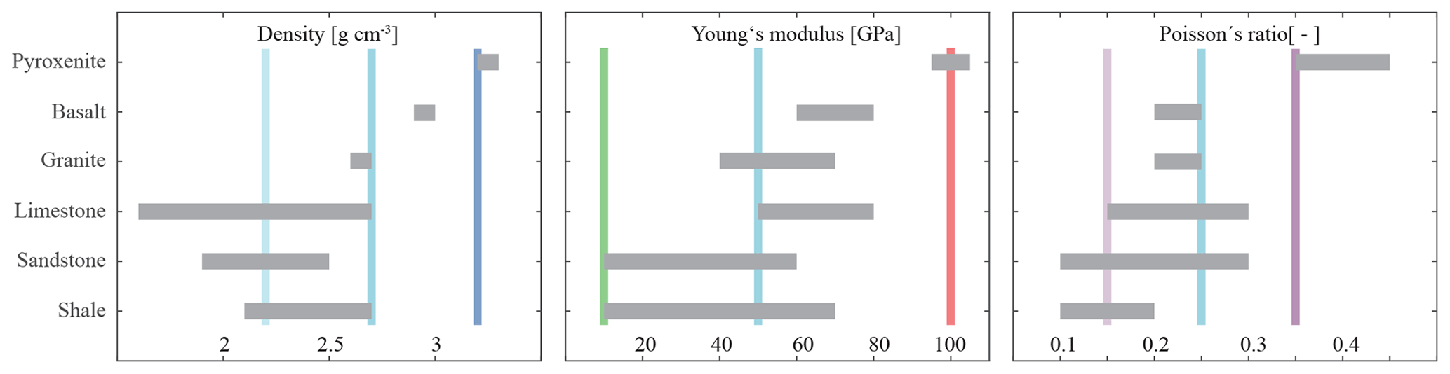
Figure 3Selection of common elastic rock properties (Young's modulus and Poisson's ratio) and density (Turcotte et al., 2014). Coloured vertical bars indicate applied material properties; see Table 2.
4.2 Solution of the equilibrium of forces
The stress orientations in the models are investigated using the finite-element method (FEM). The usage of 3-D FEM models to investigate the stress state in the crust is a well-established technique (e.g. van Wees et al., 2003; Buchmann and Connolly, 2007; Hergert and Heidbach, 2011; Reiter and Heidbach, 2014; Hergert et al., 2015). The major reason that complex 2-D or 3-D models can be computed is the opportunity to use unstructured meshes.
The method in general computes the equilibrium of stresses arising from boundary forces (via displacement boundary conditions) and body forces (gravity) acting on the rock whose mechanical behaviour is characterized by a constitutive law and associated material parameters. The equilibrium of forces is represented by partial differential equations, which are solved numerically.
where δσij is the variation of total stress, δxj is the spatial change and ρxj represents the weight of the rock section (ρ=density). Linear elastic material behaviour expressed by Hooke's law is assumed. Two material properties, Young's modulus (E) and Poisson's ratio (ν) are essential. The stress state in this study will be calculated based on defined displacement boundary conditions (Fig. 2).
The lateral resolution of the model is about 3 km, consisting primarily of hexahedrons and some wedge elements (degenerated hexahedrons). Resolution into depth ranges from 0.44 km near the surface to about 3.4 km at the base of the model. In total, about 166 000 elements were used. The model version with contact surfaces uses 1725 contact elements along each contact surface. Model discretization was performed with HyperMesh® v.2019. The equilibrium of forces (body forces and boundary condition) is computed numerically using the Abaqus®/Standard v.6.14-1 finite-element software.
4.3 Mechanical properties
The main subject of this study is to investigate the impact of the variation of elastic rock properties, density and friction along faults on stress orientation in the upper crust in the given geometrical setting outlined in the previous sections (Fig. 2). To do this, each parameter is tested individually. Figure 3 visualizes the range of density (ρ), Young's modulus (E) and Poisson's ratio (ν) of representative rocks, taken from a textbook (Turcotte et al., 2014).
The reference material for this investigation has a density of , a Poisson's ratio of ν=0.25 and a Young's modulus of E=50 GPa. Such a material could represent for example granite or limestone. Based on this reference material, a lower and higher material value is always defined (Table 2), which is within the range of common rock properties (Fig. 3). The material with a low density () may represent sediments (sandstone, limestone, shale etc.), whereas the high-density material () could represent a rock from the lower crust or the upper mantle. A low Poisson's ratio (ν=0.15) may represent sediments (sandstone or shale), and a high Poisson's ratio (ν=0.35) could represent ultramafic rocks. Soft material with a low Young's modulus (E=10 GPa) may represent sediments, pre-damaged rock or weathered rock. Again ultramafic rock is an example of a stiff rock, having a large Young's modulus (E=100 GPa).
Table 2Young's modulus, Poisson's ratio and densities used in the models. Bold numbers indicate the properties used, which differ from those of the reference material.
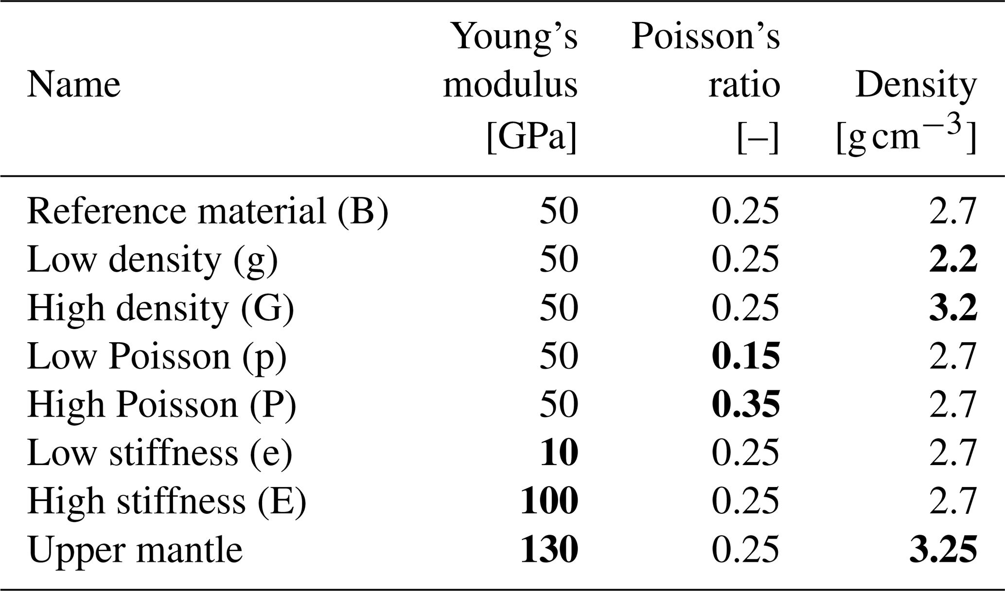

Figure 4The stress ratio k (Eq. 3) is plotted vs. depth. Stress in the reference model is marked with the bold green line. Additionally, several data and defined stress ratios from the literature are visualized for comparison (Heim, 1878; Herget, 1973; Brown and Hoek, 1978; Lindner and Halpern, 1978; McCutchen, 1982; Sheorey, 1994; Brudy et al., 1997; Hickman and Zoback, 2004).
Laboratory rock experiments in the past delivered friction coefficients of about μ=0.6 to 0.85 (Byerlee, 1978). However, recent investigations using realistic slip rates for earthquakes decreased estimated friction coefficients by 1 order of magnitude down to μ<0.1 (Di Toro et al., 2011). Faults are represented by cohesionless contact surfaces in the models. The used friction coefficients are 0.1, 0.2, 0.4, 0.6, 0.8 and 1.0, which covers both slow and fast slip rates.
4.4 Initial stress state
The present-day stress state in the crust is a complex product of several stress sources from the past to the present. In order to model the stress state an initial stress state is defined, which is in equilibrium with the body forces (gravity) and which subsequently undergoes lateral straining to account for tectonic stress. Sheorey (1994) provided a simple semi-empirical function (Eq. 2) for the stress ratio k (Eq. 3), where E is Young's modulus and z is the depth in kilometres.
Sheorey's equation (Eq. 2) is a reliable stress ratio vs. depth estimation, when compared to real-world data (Fig. 4). The model is pre-stressed with zero horizontal strain boundary conditions. The pre-stressing method used here has so far been used several times (Buchmann and Connolly, 2007; Hergert and Heidbach, 2011; Reiter and Heidbach, 2014). The model is allowed to compact several times under application of the body forces (gravity) using a Poisson's ratio of ν=0.396 during that procedure only. During the pre-stressing procedure, models with contact surfaces have a very large friction coefficient (μ=10) to prevent slip. At a virtual well in the centre of the model (x=150 km; y=200 km) stress was extracted from the model and compared to the stress magnitude data, which are visualized in Figs. 4 and 5, showing a good fit to stress–depth distribution assumptions (Heim, 1878; Herget, 1973; Brown and Hoek, 1978; McCutchen, 1982; Sheorey, 1994) and measured magnitude ratios also (Brown and Hoek, 1978; Lindner and Halpern, 1978; Brudy et al., 1997; Hickman and Zoback, 2004).
4.5 Boundary conditions
The overall SHmax orientation on a virtual profile along longitude 11∘ (Fig. 1) displays a north–south orientation in the North German Basin (NGB) and in the Molasse Basin (MB) north of the Alps, except the Variscan basement units in between. Correspondingly, a north–south orientation of SHmax is intended for the reference model. In order to generate a meaningful stress state in the model, appropriate boundary conditions are required, which are technically applied by a defined lateral displacement. Results from a virtual well in the model centre are compared with data from deep wells. An extension of 60 m () in the east–west direction and a shortening of 400 m () in the north–south direction (Fig. 2) provide a good fit of the reference model to stress magnitudes from selected deep wells (Fig. 5, Brudy et al., 1997; Hickman and Zoback, 2004; Lund and Zoback, 1999). By fitting the data, the focus was more on the observed Shmin magnitudes and to a lesser extent on the SHmax magnitudes. The latter are less reliable, as they are usually not measured; they are calculated on the basis of several assumptions. The determined boundary conditions are used for all models.

Figure 5The stress magnitudes are plotted as a function of depth. The stress components from the virtual well in the model are illustrated by the coloured lines. The location of the virtual well and boundary conditions used are shown in Fig. 2. Due to the applied initial stress conditions, the stress regime changes from thrust faulting at a depth of 400 m to strike slip faulting, and finally to a normal faulting regime at a depth greater than 5500 m. Published stress magnitude data are shown for comparison (Brudy et al., 1997; Lund and Zoback, 1999; Hickman and Zoback, 2004).
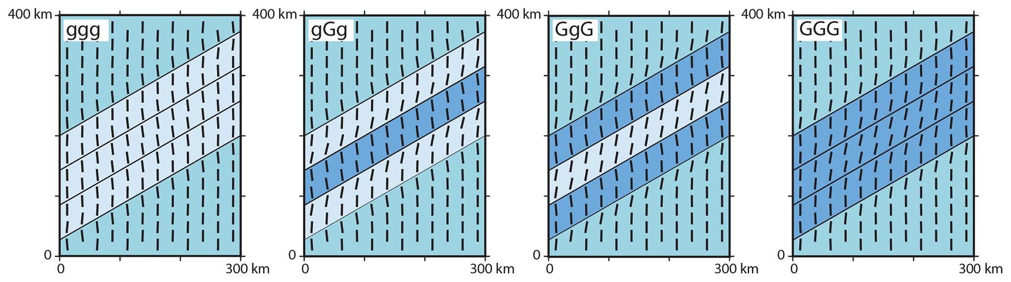
Figure 6Influence of density on the stress orientation. Black bars represent the orientation of SHmax at a depth of 1000 m. Colours indicate the material properties used. The medium blue area uses the reference material properties (), the light blue material uses a lower density (g: ), the dark blue a larger density (G: ).
4.6 Generic model scenario's
The model geometry consists of five units (Fig. 2). The northern- and southernmost blocks are always assigned the reference material properties (Table 2). In between there are three diagonal units in which material properties are varied. Along the vertical borders within the model, friction properties can be used. The lower (L) or higher (H) values of the material properties with respect to the reference material (B) will be varied in the following way: LLL, HHH, LBL, BLB, etc. When the model geometry mimics discontinuities using contact surfaces, all contacts have the same friction coefficient. In the figures showing the results the label “|” indicates contact. For example, HLH with four contacts is |H|L|H|.
The SHmax orientation is visualized at a depth of 1000 m below the surface using a pre-defined grid, where the lateral distance to the material transition or discontinuity is >12.5 km, as far-field effects are the main interest of this study. The variation of density, Poisson's ratio, Young's modulus and friction coefficient will be tested first. In addition, the variation of Young's modulus is tested in interaction with low-friction contacts.
Table 3Material properties used for the scenario using realistic rock properties for Variscan basement units; properties are estimated based on Turcotte et al. (2014). MGCH = Mid-German Crystalline High, MZ = Moldanubian Zone, NPZ = Northern Pyllite Zone, RHZ = Rheno-Hercynian Zone, STZ = Saxo-Thuringian Zone.

4.7 Realistic rock property scenario
A reality-based rock property scenario, inspired by the structural zonation of the European Variscides according to Kossmat (1927), is tested. The RHZ and the NPZ are dominated by clastic shelf sediments with a low- or mid-metamorphic overprint, which is made of slate (RHZ) and phyllite (NPZ). This zone, the RHZ and the NPZ together, is the most flexible one and will have the lowest Young's modulus (Table 3). The MGCH consists of granitoids or gabbros and their metamorphic equivalents (gneiss, amphibolite), meta-sediments, and some volcanites. Therefore, this zone is a stiff unit. The Saxo-Thuringian Zone (STZ) is dominated by meta-sediments, mafic and felsic magmatites and their metamorphosed equivalents, and some high-grade metamorphic rocks (granulite, eklogite). Taking all the different rock types into account, the STZ is stiffer than the RHZ and softer than the MGCH. Mechanically, the MZ can be represented by high-grade metamorphic rocks (gneiss, granulite, migmatite) and granitoids and will be a stiff unit, similar to the MGCH. Therefore, the unit stiffnesses are different: they are from slightly deformable to rigid in the following order: . Material properties used are estimated based on typical rock values (Table 3). The same initial stress procedure, boundary condition and visualization procedure are applied as previously described.
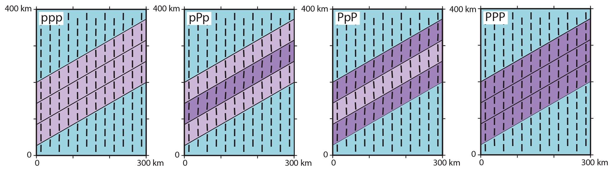
Figure 7Influence of Poisson's ratio on the stress orientation. Black bars represent the orientation of SHmax at a depth of 1000 m. Colours indicate the material properties used. The blue area uses the reference material properties (ν=0.25), the light purple area is characterized by a low Poisson's ratio (p: ν=0.15) and the dark purple one by a large Poisson's ratio (P: ν=0.35).
5.1 Density influence
To identify the influence of a density variation, the reference density () in blue is varied using a small density (g: ), which is coloured in light blue, and a large density (G: ), which is dark blue (Fig. 6).
The low-density anomaly (ggg) results in a slight counter-clockwise () rotation of the SHmax orientation in the reference material near the anomaly (Fig. 6). Within the low-density units near the reference material, nearly no rotation is observed (), but SHmax orientation turns counter-clockwise () in the centre of the material anomaly. The angular variation of SHmax crossing the units is of the order of 7∘. The high-density anomaly (GGG) results in a slightly clockwise rotation () in the reference material near the anomaly. In the high-density unit near the reference material, SHmax is minimally influenced () but rotates further clockwise () in the centre of the anomaly. Based on that, the variation across the units is about 11∘. The models with mixed densities in the three units show a clockwise rotation () of SHmax within the lighter material next to the denser units. The high-density units show a counter-clockwise rotation () next to the low-density unit; therefore, the total variation of SHmax is 17∘.
In general, SHmax tends to be oriented parallel to the anomaly in low-density units and perpendicular to the anomaly in large density units. In the centre of the low-density units (ggg), the stress orientation becomes perpendicular to the overall structure. In the centre of the high-density units (GGG) the opposite is true, and SHmax becomes parallel to the structure.
5.2 Influence of Poisson's ratio
The influence of Poisson's ratio on the stress rotation is tested by variation of the reference Poisson's ratio (ν=0.25) using a lower one (p: ν=0.15) in light purple and a larger one (P: ν=0.35) in dark purple (Fig. 7). The models with only a lower (ppp: −1.5∘) and only a higher Poisson's ratio (PPP: +2.2∘) show only little SHmax rotation (Fig. 7). Mixed models with largest Poisson's ratio variation (pPp and PpP) have some counter-clockwise rotation in the low Poisson's ratio units () and a clockwise rotation in the high Poisson's ratio units (). Therefore, the total variance of SHmax is about 7.5∘.
5.3 Impact of Young's modulus

Figure 8Influence of Young's modulus variation on the stress orientation. Black bars represent the orientation of SHmax at a depth of 1000 m. Colours indicate the used Young's modulus; the blue area uses the reference material properties (B: E=50 GPa), the green material uses a low Young's modulus (e: E=10 GPa) and the red material has a large Young's modulus (E: E=100 GPa).
The impact of Young's modulus is investigated using the reference material (B: E=50 GPa) in contrast to a softer material (e: E=10 GPa) in green and a stiffer material (E: E=100 GPa) in red (Fig. 8). The models with the soft units (eee, eBe and BeB) exhibit a strong clockwise SHmax rotation (+56∘) in the units with the reference material and a counter-clockwise rotation in the softer units (−22∘) near the material transitions. For the models with three soft units (eee) the SHmax orientation decreases to −5∘ in the centre of the units. This means that the SHmax variation within the soft units is considerable (17∘). The resulting total variation is 78∘. The models with the stiff units (EEE, EBE and BEB) exhibit a gentle counter-clockwise rotation in the units with the reference material (−5.5 to −7∘) next to the stiff units. Within the stiff units, a significant clockwise rotation (+20 to +25∘) is apparent next to the reference units. In the model with three stiff units (EEE), the SHmax orientation decreases to (+5∘) in the centre. This is a considerable SHmax variation of 15∘ within the stiff units. The total variation is 31∘.
For the models with alternating soft and stiff material units (EeE and eEe), the soft units exhibit a counter-clockwise SHmax rotation (−19 to −22∘), whereas the stiff units display a clockwise rotation (+53 to +56∘). Consequently, the total variation between the soft and stiff units is 72 to 78∘. The general observation is that next to the material transition, SHmax rotates perpendicular to the anomaly for the compliant units and parallel for the stiff units.
5.4 Influence of faults
Several models with the reference material properties separated by three discontinuities (|B|B|B|) with a friction coefficient (μ) from 0.1 to 1 are tested. The low-friction coefficient (μ=0.1) leads to a counter-clockwise SHmax rotation of only −3∘ (Fig. 9). The maximum observed fault offset is about 16 m. By increasing the friction coefficient to μ=0.2, the SHmax rotation is −2∘; for μ=0.4, SHmax rotation is only −1∘. For larger friction coefficients, the SHmax rotation is below . As the SHmax rotation is too small for a visual differentiation, only the μ=0.1 model is shown in Fig. 9.
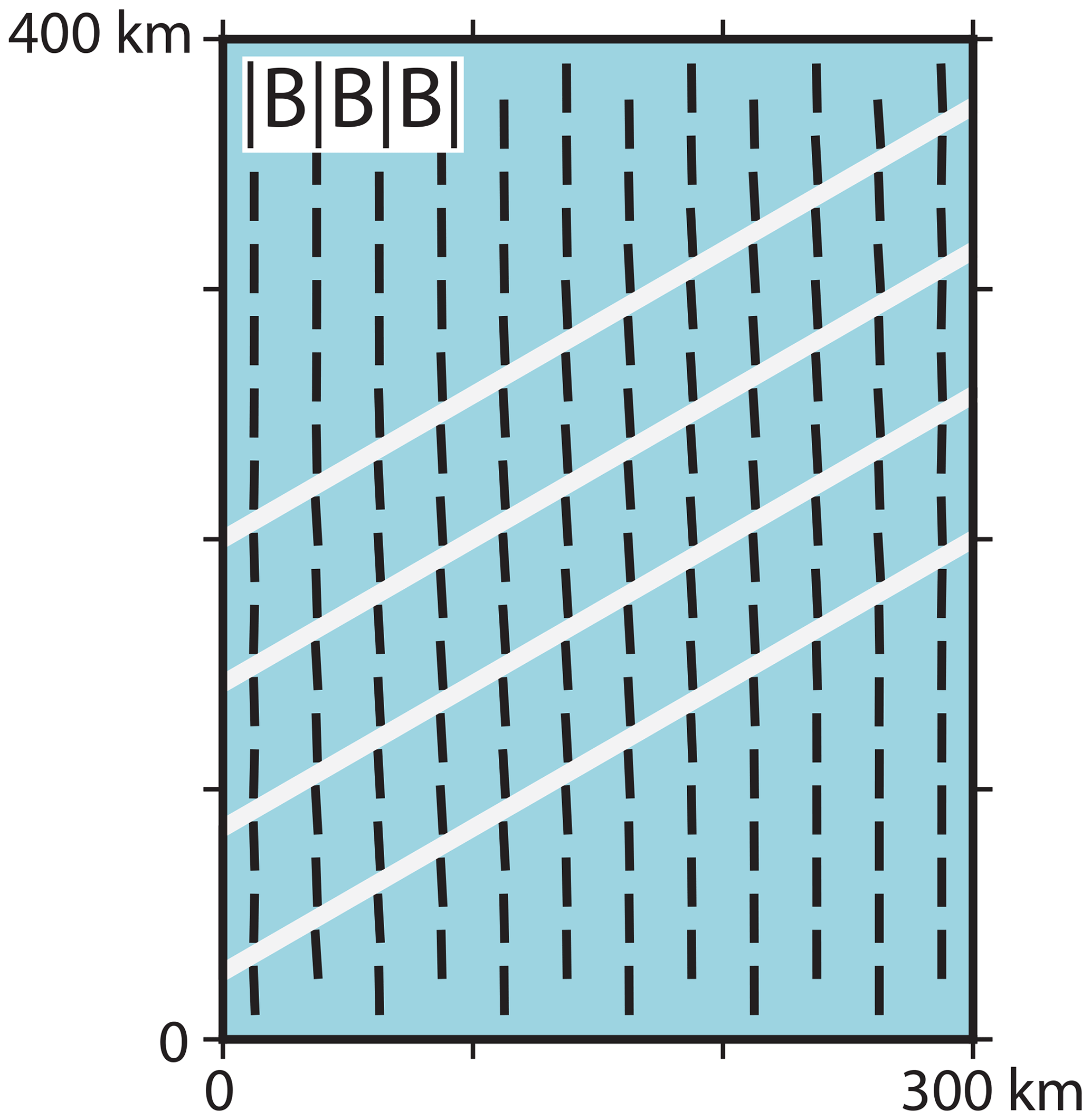
Figure 9Influence of low-friction faults on the far-field stress orientation. Black bars represent the orientation of SHmax at a depth of 1000 m. All areas have the properties of the reference material (Table 2). White lines indicate cohesionless discontinuities (vertical faults). The model using a friction coefficient of μ=0.1 along the three discontinuities is shown. The other models with a larger friction coefficient (up to 1 and larger) have similar results; they are waived out because of the visual similarity.
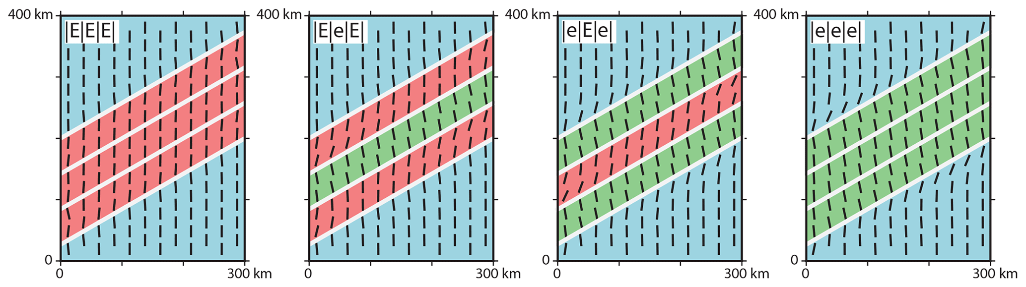
Figure 10Influence of Young's modulus in interaction with low-friction faults on the far-field stress orientation. Black bars represent the orientation of SHmax at a depth of 1000 m. Colours indicate the material properties used. The blue area uses the reference material properties, the green material uses a low Young's modulus and the red material has a larger Young's modulus; see Table 2. White lines indicate cohesionless vertical discontinuities (faults) with a friction coefficient of μ=0.1.
5.5 Stiffness variation combined with low-friction faults
The interaction between a significant Young's modulus contrast and a cohesionless contact with a low-friction coefficient (μ=0.1) is tested along all four discontinuities. The model with three stiff units (|E|E|E|) provides only little counter-clockwise rotation () in the reference material near the material transition (Fig. 10). Similar clockwise rotation occurs in the stiff units () near the material transition and decreases to the centre of the units (). The total SHmax variation is about 8∘.
The model with the soft units and the low-friction discontinuities (|e|e|e|) shows larger rotations than the model with stiffer units. Clockwise rotation of +19∘ occurs in the reference material and counter-clockwise rotation of −13∘ in the soft units. This decreases towards the centre of the soft units (−9∘). Overall rotation is about 32∘.
The models with alternating stiffnesses and low-friction discontinuities (|E|e|E| and |e|E|e|) generate a counter-clockwise rotation of about −10 to −12∘ in the soft units. Within the stiff units, the SHmax orientation is in the range of +2 to +7∘. The total variation is up to 19∘. The maximum observed fault offset is about 10 to 15 m.
5.6 Stress rotation for realistic material properties
The resulting SHmax orientation (Fig. 11a) of the model using realistic material properties (Table 3) indicates counter-clockwise rotation in the RHZ and NPZ and clockwise rotation within the MGCH and MZ units. The overall pattern of the simple model (Fig. 11a) shows only limited similarity with the observed and the mean SHmax orientation on a regular grid using a search radius of 150 km and a quality and distance weight (Fig. 11b and c). However, some similarities can be observed. For example, the simple model (Fig. 11a) shows a clockwise rotation from the NPZ to the MGCH and counter-clockwise from the MGCH to the STZ. In Figure 11b these areas show similar, but less pronounced, rotation of SHmax. The north-north-east SHmax orientation within the central part of the MGCH is similar between the model, the data and the mean SHmax orientation (Fig. 11a–c).
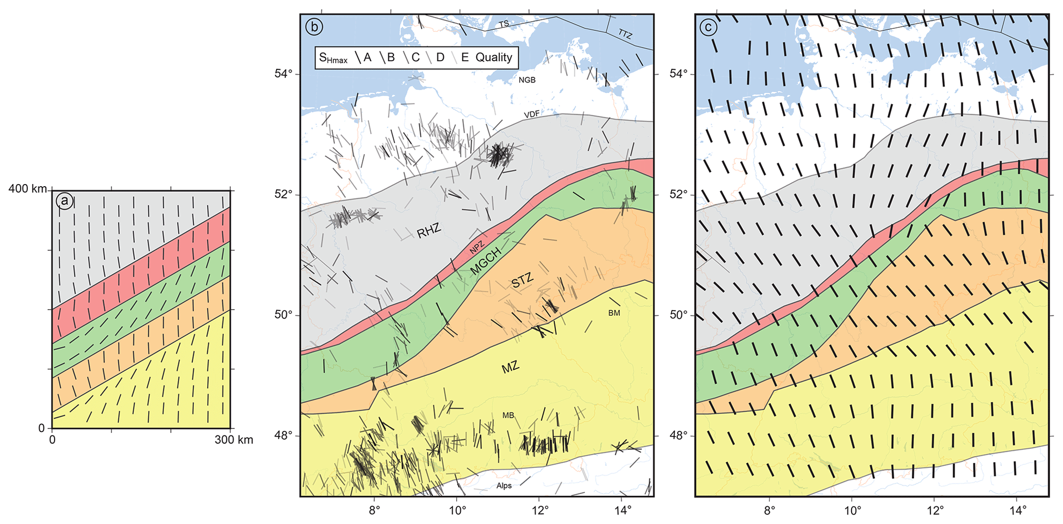
Figure 11Comparison of orientations of the maximum horizontal stress (SHmax). The equivalent regions are the RHZ (Rheno-Hercynian Zone), NPZ (Northern Phyllite Zone), the MGCH (Mid-German Crystalline High), the STZ (Saxo-Thuringian Zone) and the MZ (Moldanubian Zone). (a) Model results, application of estimated material properties of the Variscan units (Table 3). Black bars represent the SHmax orientation at a depth of 1000 m. (b) Bars indicate the SHmax orientation data (Heidbach et al., 2018), and quality is indicated by shades of grey; see legend. (c) Mean SHmax orientation on a 150 km search radius with a distance and quality weight (n>3) using the tool stress2grid (Ziegler and Heidbach, 2017). Panels (b) and (c) have the same extent as Fig. 1.
6.1 Model simplification
This study investigates the influence of elastic material properties, density and friction coefficient at vertical faults on the orientation of SHmax. The focus is not on stress rotation close to the material transition or discontinuity (<10 km), the priority is on the far-field effects (>10 km). Although the model is inspired by a particular region, the goal is to gain a better understanding on how the variable material properties affect the stress orientation. For this reason, the model geometry is very simple and some of the material properties used may have no proper natural equivalent.
Chosen properties are constant over a depth of 30 km, which is unlikely. Even for a given lithology, the properties can change with depth, as a result of the acting gravity and compaction, especially for sediments. Each lithological unit is at least partially affected by these changes. Linearly increasing rock properties with depth would account for this and be a more realistic representation. But this would not affect the resulting stress pattern, especially since a vertically uniform stress field is assumed (Zoback et al., 1989; Zoback, 1992; Heidbach et al., 2018), with a few exceptions.
The simple generic models neglect various rheological processes in the crust by applying linear-elastic material law. However, the overall geometry seems reasonable, as the brittle domain or elastic thickness of the lithosphere (Te), which is a measure of the integrated stiffness of the lithosphere, is of the order of 30 km and more in central Europe (Tesauro et al., 2012). The Moho depth in Germany or central Europe is also about 30 km (Aichroth et al., 1992; Grad and Tiira, 2009). Jarosiński et al. (2006) for example used a range of Te=30–100 km for their model of central Europe. Furthermore, results are represented and discussed mainly for a depth of 1000 m where elastic behaviour is certainly predominant.
The scenario models were tested with an additional very stiff mantle (Table 3) with a thickness of 30 km. This had no influence on the observed stress pattern at a depth of 1000 m. However, the models with the same geometry but a total thickness of only 10 km resulted in much lower stress rotation. Therefore, the elastic thickness of the lithosphere and the aspect ratio of thickness and width of the units are important constraints for the possible stress rotation. The depth at which the stress orientation is plotted is also important, as the stress rotation decreases with depth (Fig. 12), so that it disappears at about 10 km depth for the used configuration. As homogeneous material properties are used, smaller scaling of results seems to be reasonable, considering the aspect ratio.
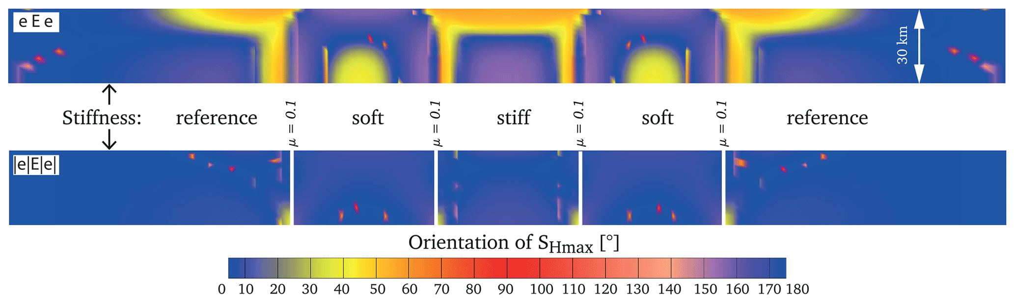
Figure 12North–south depth profiles displaying the SHmax orientation colour-coded for models with a variable Young's modulus. In the model without the discontinuities (eEe), SHmax is oriented around 40∘ in the stiffer units next to the softer units near the Earth surface. A similar orientation can be observed in the soft units in the deepest parts. In contrast to that, in the model with the same material properties but low-friction faults (|e|E|e|), the SHmax orientation is nearly north–south for all units and depths. (Small coloured dots are artefacts.) The discontinuities with a low-friction coefficient counterbalance stress rotation due to the stiffness contrasts.
All models were loaded with the same displacement boundary conditions (Fig. 2). This results in slightly different stress magnitudes due to the variable material properties. Since these models have different mechanical properties depending on the unit, the question would arise, in which of the units identical stress magnitudes should be achieved? Even if each model were calibrated individually, this would not significantly change the results, as both the stress regime and stress orientation would remain nearly constant for slightly different boundary conditions. Therefore, constant boundary conditions are reasonable and applied to all scenarios.
6.2 Stress rotation by density contrast
The lateral variation of the density is responsible for SHmax rotation in the range of 7 to 17∘ (Fig. 6). In general, the SHmax rotates in the low-density units slightly toward parallel to the high-density unit (+10∘), whereas SHmax rotates in the high-density units a little bit in the direction to the low-density units (−7∘).
Taking a broad range of sediments into account (evaporites, shale, sandstone or limestone), they could have even a lower density than the lowest value used (). Most probably, models with a lower stiffness would result in larger stress rotation. However, sediments with a low stiffness could reach a thickness of several thousand metres, but not of the order of the model depth of 30 km or with such a low density due to increasing compaction with depth. Therefore, the impact of density variation on the stress orientation in nature will be much smaller, or on a very local scale. This agrees with the results of Gölke and Coblentz (1996), where a lateral density variation did not have a significant impact on the stress pattern; only local effects are observed.
This assumption seems to be a contradiction to the fact that the gravitational load is one of the main sources of stress in the Earth's crust. However, a density anomaly is a much smaller influencing variable on the stress state than density. According to Sonder (1990), the resulting stress rotations depend on the relative influence of regional stress sources as opposed to the density anomaly. Depending on the model scenarios used, the influence of the boundary conditions (regional stress sources) appears to be greater than that of the density anomaly. Therefore, the model results are probably not representative for regions with small horizontal differential stresses.
6.3 Stress rotation due to a variation of Poisson's ratio and Young's modulus
Model results suggest that the variation of Poisson's ratio can be responsible for a SHmax rotation of up to 7.5∘ (Fig. 7). This is below the uncertainties of stress orientation estimations of about ±15∘ and more (Heidbach et al., 2018). Therefore, the variation of Poisson's ratio can be neglected as a potential source of significant stress rotation.
In contrast to that, the lateral variation of Young's modulus can lead to significant SHmax rotation (Fig. 8). For the geometry and material parameters used, the relative rotations are up to 78∘, which is not far from the maximal possible rotation of 90∘. The largest rotation occurs in the units with a lower Young's modulus, for example the eee model has a total rotation of 78∘, whereas the EEE model causes only a 31∘ rotation. This is not surprising as Young's modulus is simply a measure of the stiffness. Therefore, the largest stress rotation due to stiffness contrast will happen in the soft units, not in the rigid ones. From this, it can be deduced that for units with smaller Young's modulus, the stress rotation is even greater.
SHmax will be oriented parallel to the structure for stiff units and perpendicular for soft units, which agrees with the literature (Bell, 1996; Zhang et al., 1994). The largest stress rotation occurs nearest to the material transition and decreases with distance to the material transition, similar to other models (Spann et al., 1994). Similar impacts of stiffness contrast have been described in previous studies (Grünthal and Stromeyer, 1992; Spann et al., 1994; Tommasi et al., 1995; Mantovani et al., 2000; Marotta et al., 2002). In contrast to that, Jarosiński et al. (2006) found that a stiffness contrast has only minor effects. But they did not test the stiffness contrast separately; they applied it only in combination with active faults in between the units. However, this agrees with the results of this study, as active faults balance stress rotation by stiffness contrast.
Within the units with a small Young's modulus, significant deformation is possible. For example, within the eEe model (Fig. 8), the soft units in green will be sinistrally deformed. The stiff unit in red cannot be deformed in the same way. But as the units are connected, the stiff unit is affected by the tangentially acting stress source. This leads to a SHmax orientation parallel to the structure, within the stiff units. As the soft one allows such deformation, SHmax will be oriented normally to the stiff unit.
At the interface between stiff and soft units differential stresses are greatest, as both units are differently deformable. This fits with the observation of concentrated intra-plate earthquakes around cratons (Mooney et al., 2012). On a smaller scale this has been observed for stiff sedimentary layers or rigid dykes, which attracts the occurrence of seismicity (Roberts and Schweitzer, 1999; Ziegler et al., 2015).
The observed radial stress pattern to the south of the Bohemian Massif (Reinecker and Lenhardt, 1999) agrees well with this study, where SHmax in the soft sediments of the Upper and Lower Austrian basin is perpendicular to the stiff crystalline Bohemian Massif. This is more ambiguously the case for the fan-shaped pattern in the western and northern part of the Alpine molasse basin (Grünthal and Stromeyer, 1992; Kastrup et al., 2004; Reinecker et al., 2010). The reason for this could be a lateral stiffness contrast of the rock, next to the topographic features of the mountain chain and the overall crustal structure. When comparing the stress rotation, it is important to consider the respective depth (see Fig. 12). For example, data in the north-western Alps originate from focal mechanisms, and in the foreland of the central Alps, the majority of data are from wells, which are more shallow (Reinecker et al., 2010).
Substantial stress rotations are not observed along major pre-Mesozoic boundaries and sutures in the eastern United States, like the Greenville front, a suture from Missouri to New York, or in the Appalachian Mountains (Zoback, 1992). Gregersen (1992) reports the same for Fennoscandia. In the case that these tectonic boundaries did not provide a significant stiffness transition, it is not a contradiction to this study. The mechanical contrast is important, not the relative ages.
6.4 Comparison of stress rotation due to elastic material properties
The rotation of SHmax perpendicular (counter-clockwise) to the structure can be observed most clearly in material with a lower Young's modulus next to a material transition, up to −22∘. Rotation in the same direction, but with a lower amount, is observed in rocks with a larger density or a smaller Poisson's ratio. Within the units with a greater Young's modulus, SHmax rotates significantly parallel (clockwise) to the material transition, up to 56∘. Similar rotation with a smaller magnitude can be observed in the low-density units or in the units with a larger Poisson's ratio. As rocks with a larger Young's modulus will usually have a larger density and vice versa (Fig. 3), real rocks will have less SHmax rotation as suggested by these generic models. But the aim of this study is to test and combine the possible range of variation, in order to identify the most important causes (Fig. 13).

6.5 Failure criteria
As only elastic material properties are used, failure is not possible. To study the influence of this simplification, two models (EEE and eee) have been calculated using two different Coulomb failure criteria. The models are run first with a cohesion (C) of 30 MPa and a friction angle (FA) of 40∘ and in addition with C=10 MPa and a FA of 30∘.
For the EEE model with C=30 MPa and FA = 40∘, no failure will be reached (yield criteria <1). For the eee model using that criteria and for both models (EEE and eee) using C=10 MPa and FA = 30∘ failure occurs. Conditions of failure or close to failure (Yield criteria ∼1 or >1) occur only near the surface (a few kilometres) and close to the material transition (∼20–30 km). Around the material transition, (near) failure can be observed within the stiff units only. For the EEE model with C=10 MPa and FA = 30∘, failure is more spaciously distributed near the surface.
In the case of failure, the SHmax orientation will be balanced, which means that SHmax rotates back in the north–south orientation, similar to the applied boundary conditions. In general, failure compensates for stress rotation in the same way as low-friction contact surfaces (faults). However, the stress orientation in the models that account for failure shows a similar stress pattern in the pre-failure phase to the models without failure. As a conclusion from this observation, the model results showing significant stress rotation are still valid for solid rocks.
6.6 Effect of faults on stress orientation
According to the model results, the influence of low-friction faults can be neglected concerning the orientation of the far-field stress pattern for homogeneous units. The low-friction faults (C=0, μ=0.1; FA 5∘) lead to only 3∘ SHmax rotation at a distance of about 12.5 km next to the fault zone. Observed stress rotation is lower than 1∘ for a friction coefficient μ>0.4. This is not in contrast to the strong stress perturbation, observed in the vicinity of faults; as one of the three principal stresses must be oriented perpendicular to a fault, the two remaining ones are parallel to the discontinuity (Bell et al., 1992; Bell, 1996; Jaeger et al., 2007). Observations from meso-scale outcrops indicate stress perturbation within 2 km (Petit and Mattauer, 1995) or less than 1 km to a fault (Rispoli, 1981); larger stress perturbation can be observed at the termination of the fault (2–3 km). If SHmax is parallel next to the fault, it will rotate by 90∘ at the termination of the fault (Rispoli, 1981; Osokina, 1988).
Yale (2003) suggests significant stress rotation as a product of active faults within a distance of several hundred metres for large differential stress provinces and several kilometres for regions with small differential stresses. This is supported by observed stress rotations near a fault within a range of a few hundred metres to a few kilometres (Brudy et al., 1997; Yassir and Zerwer, 1997). However, not all observed stress rotation agrees with the presented models, like observations offshore of eastern Canada (Bell and McCallum, 1990; Adams and Bell, 1991), where stress rotation occurs at a distance of about 10–15 km to a fault. Whether this is due to an inaccurate localization of the fault, a low Young's modulus or other causes cannot be clarified here.
Numerical models investigating stress rotations near a fault provide stress rotation between 20 and 60∘, next to the fault, depending on the fault strike, the boundary conditions, and the friction or weakness of the fault. Near the termination of the fault, stress rotation increases to 50–90∘ (Zhang et al., 1994; Tommasi et al., 1995; Homberg et al., 1997). However, rotation is observed by these models only within 2–3 elements, away from the discontinuity, which are anyway needed to distribute the deformation by such numerical models. Therefore, observed distances of rotation within these models are not considered here. To avoid this influence of an overly coarse mesh, the orientation of SHmax in this study is displayed at least four elements away from the contact surface.
6.7 Effect of faults combined with stiffness contrasts on stress orientation
The models with low-friction faults and a variable stiffness (Fig. 10) illustrate much lower stress rotation than the models without the faults (Fig. 8). The reason is that the soft units cannot transfer tangential shear stresses to the stiffer units. Therefore, each unit can be deformed independently from each other.
It seems to be that discontinuities play an important role in reducing stress rotations, produced by lateral Young's modulus variation (or other reasons). Regarding the used model geometry and materials, the SHmax variation is reduced for the soft models from 78 to 32∘, for a comparison of eee and |e|e|e| in Figs. 8 and 10, using a friction coefficient of μ=0.1. Also for the mixed models, a reduction from 78 to 19∘ is significant. Much lower is the rotation for the stiff model, with a reduction from 31 to 8∘ (EEE in contrast to |E|E|E|).
The influence of low-friction faults in combination with variable mechanical properties was also investigated for the models with a density contrast. The observed effects are limited; therefore, presentation of the results is omitted.
6.8 Depth variation
The interaction of units with a variable Young's modulus and presence or non-presence of low-friction faults is visible in Fig. 12. While the model without active faults displays significant stress rotation, the same setting with low-friction faults shows only little rotation. The observed stress rotation within the model without faults strongly depends on the depth. In the soft units, SHmax rotates counter-clockwise near the surface (0 to −8 km). In contrast to that a clockwise rotation can be observed at greater depth (18–30 km). The stiffer units show a clockwise rotation in the upper part, about 0 to −8 km, which changes slightly to a counter-clockwise orientation in the deeper part.
This could be an indication that stress rotations due to stiffness contrasts in or near sedimentary basins can be significantly greater than in deeper material transitions, such as in a buried crystalline basement. This is all the more likely as sediments tend to be less stiff than crystalline rock.
6.9 Model using the Variscan zone rock properties
Figure 11 presents comparatively the results of SHmax orientation of the model using the chosen material properties, inspired by the Variscan units (a), the SHmax orientation data (b) and the averaged orientation of SHmax on a regular grid (c). A limitation of the mean stress orientation on a regular grid (Fig. 11c) is the calculation based on distance, and not depending on the specific unit. The similarity of the SHmax orientation is not very convincing, because the overall pattern cannot be reproduced. Some of the deviations from the trend are similar, some are not.
There are probably several reasons why the simple model is not able to reproduce the observed stress pattern in the German Variscides (Fig. 11). First of all, only one single elastic material composition represents each of the Variscan units. The model did not reproduce the complex and uncertain vertical variability of the deeper structures (Franke et al., 1990; Aichroth et al., 1992; Blundell et al., 1992), as no deep wells are present there. Only refraction seismic profiles from the 1980s (DEKORP) and their interpretations are available (Meissner and Bortfeld, 1990). Consequently, besides the uncertain structures, the material properties and the dip of the unit boundaries are also uncertain. More complex geometries and variable dip angle may result in different stress patterns to the ones obtained for vertical discontinuities. However, studying such variability is beyond the scope of this study.
Of course, it could also be possible that the units are decoupled. Thus, a scenario was calculated in which the units are separated by low-friction faults. But this did not provide a better fit of the stress orientation in contrast to the observation. Furthermore, there are no seismic or geodetic indications for such a decoupling of the units in that region.
Structures outside the Variscan zonation may also play a role. To the south, the stress pattern in the Molasses Basin is probably more governed by the structure of the Alpine chain (Reinecker et al., 2010) than older structures. The fan-shaped stress pattern in the eastern part of the North German Basin has been explained as an effect of the close boundary to the stiff Eastern European Craton along the north-west to south-east striking TTZ (Grünthal and Stromeyer, 1986, 1992, 1994; Gölke and Coblentz, 1996; Goes et al., 2000; Kaiser et al., 2005; Marotta et al., 2002). This interpretation agrees well with the results of the models, where SHmax becomes perpendicular in a soft unit (NGB) directed to a stiff region, like the East European Craton (e.g. model eee in Fig. 8).
The effect of varying elastic material parameters (Young's modulus and Poisson's ratio), density and low-friction discontinuities on the stress pattern in map view is investigated. Each property is tested separately to avoid interdependencies. This is performed with generic 3-D models using the finite-element method. Three units of variable material properties are included within the models, with boundary conditions determining the overall SHmax orientation. The variation of density and Poisson's ratio lead to small rotation (17 and 7.5∘) of SHmax. In contrast, stiffness variation is able to produce significant stress rotation of 31 to 78∘. Therefore, variation of Young's modulus in the upper crust is a potent explanation for observed stress rotation. Faults are represented in the models by cohesionless contact surfaces. The observed stress rotation in the far field due to low-friction faults (μ=0.1) is less than 3∘. Implementation of low-friction discontinuities in models with a Young's modulus anomaly results in much smaller SHmax rotation, of the order of 8 to 32∘. It follows that faults do not produce far-field stress rotation, but rather compensate for stress rotation that is an effect of the Young's modulus anomaly or other causes. Comparison of the model results with the observed stress orientation in the region that inspired the models provides only limited consistency. Nevertheless, the studies clearly show that fault systems are hardly the source of stress rotations on length scales of 100 km or larger. Furthermore, the study indicates that strength contrasts are promising candidates that have the potential to explain the slight stress pattern rotations in intraplate settings where topography and low-friction fault systems are missing.
Model discretization was performed with the commercial software HyperMesh® v.2019; the equilibrium of forces is computed numerically using the commercial software Abaqus®/Standard v.6.14-1. Model input files are available online at https://doi.org/10.48328/tudatalib-560 (Reiter, 2021). Maps and model illustrations (except Fig. 12) were generated using Generic Mapping Tools (GMT) software (Wessel et al., 2013).
Stress orientation data are available online at https://doi.org/10.5880/WSM.2016.001 (Heidbach et al., 2016).
The author declares that there is no conflict of interest.
I want to thank Oliver Heidbach, Tobias Hergert, Birgit Müller and Moritz Ziegler for fruitful discussions about mechanics in the upper crust and the observed stress rotation pattern as well as comments on the paper. Also I would like to thank two anonymous reviewers for their constructive annotation, which improved the paper.
This research has been supported by the Federal Ministry for Economic Affairs and Energy (BMWi) (grant no. 02E11637A). This study is part of the SpannEnD Project (http://www.SpannEnD-Projekt.de, last access: 8 June 2021).
This paper was edited by David Healy and reviewed by two anonymous referees.
Adams, J. and Bell, J. S.: Crustal Stresses in Canada, in: Neotectonics of North America, chap. 20, Geological Society of America, Boulder, Colorado, 367–386, 1991. a, b, c
Ahlers, S., Henk, A., Hergert, T., Reiter, K., Müller, B., Röckel, L., Heidbach, O., Morawietz, S., Scheck-Wenderoth, M., and Anikiev, D.: 3D crustal stress state of Western Central Europe according to a data-calibrated geomechanical model – first results, Solid Earth Discuss. [preprint], https://doi.org/10.5194/se-2020-199, in review, 2020. a
Aichroth, B., Prodehl, C., and Thybo, H.: Crustal structure along the Central Segment of the EGT from seismic-refraction studies, Tectonophysics, 207, 43–64, https://doi.org/10.1016/0040-1951(92)90471-H, 1992. a, b
Anderson, E. M.: The dynamics of faulting, Transactions of the Edinburgh Geological Society, 8, 387–402, https://doi.org/10.1144/transed.8.3.387, 1905. a
Anderson, E. M.: The Dynamics of Faulting and Dyke Formation with Application to Britain, 2nd edn., Oliver and Boyd, London and Edinburgh, 1951. a
Artyushkov, E. V.: Stresses in the lithosphere caused by crustal thickness inhomogeneities, J. Geophys. Res., 78, 7675–7708, https://doi.org/10.1029/JB078i032p07675, 1973. a, b
Assameur, D. M. and Mareschal, J.-C.: Stress induced by topography and crustal density heterogeneities: implication for the seismicity of southeastern Canada, Tectonophysics, 241, 179–192, https://doi.org/10.1016/0040-1951(94)00202-K, 1995. a
Bada, G., Cloetingh, S., Gerner, P., and Horvâth, F.: Sources of recent tectonic stress in the Pannonian region:inferences from finite element modelling, Geophys. J. Int., 134, 87–101, https://doi.org/10.1046/j.1365-246x.1998.00545.x, 1998. a
Bell, J. S.: In situ stresses in sedimentary rocks (part 2): Applications of stress measurements, Geosci. Can., 23, 135–153, 1996. a, b, c, d
Bell, J. S. and Lloyd, P. F.: Modelling of stress refraction in sediments around the Peace River Arch, Western Canada, Current Research, Part D, Geological Survey of Canada, 89, 49–54, 1989. a, b, c
Bell, J. S. and McCallum, R.: In situ stress in the Peace River Arch area, Western Canada, B. Can. Petrol. Geol., 38, 270–281, 1990. a, b, c
Bell, J. S., Caillet, G., and Adams, J.: Attempts to detect open fractures and non-sealing faults with dipmeter logs, Geol. Soc. Spec. Publ., 65, 211–220, https://doi.org/10.1144/GSL.SP.1992.065.01.16, 1992. a, b
Blundell, D. J., Freeman, R., Müller, S., Button, S., and Mueller, S.: A continent revealed: The European Geotraverse, structure and dynamic evolution, Cambridge University Press, Cambridge, https://doi.org/10.1017/CBO9780511608261, 1992. a
Bott, M. and Dean, D. S.: Stress Systems at Young Continental Margins, Nature Physical Science, 235, 23–25, https://doi.org/10.1038/physci235023a0, 1972. a
Brown, E. T. and Hoek, E.: Trends in relationships between measured in-situ stresses and depth, Int. J. Rock Mech. Min., 15, 211–215, https://doi.org/10.1016/0148-9062(78)91227-5, 1978. a, b, c
Brudy, M., Zoback, M. D., Fuchs, K., Rummel, F., and Baumgärtner, J.: Estimation of the complete stress tensor to 8 km depth in the KTB scientific drill holes: Implications for crustal strength, J. Geophys. Res.-Sol. Ea., 102, 18453–18475, https://doi.org/10.1029/96JB02942, 1997. a, b, c, d, e
Buchmann, T. J. and Connolly, P. T.: Contemporary kinematics of the Upper Rhine Graben: A 3D finite element approach, Global Planet. Change, 58, 287–309, https://doi.org/10.1016/j.gloplacha.2007.02.012, 2007. a, b
Byerlee, J.: Friction of Rocks, Pure Appl. Geophys., 116, 615–626, https://doi.org/10.1007/BF00876528, 1978. a
Coblentz, D. D. and Richardson, R. M.: Statistical trends in the intraplate stress field, J. Geophys. Res., 100, 20245, https://doi.org/10.1029/95JB02160, 1995. a
Cornet, F. H. and Röckel, T.: Vertical stress profiles and the significance of “stress decoupling”, Tectonophysics, 581, 193–205, https://doi.org/10.1016/j.tecto.2012.01.020, 2012. a
Di Toro, G., Han, R., Hirose, T., De Paola, N., Nielsen, S., Mizoguchi, K., Ferri, F., Cocco, M., and Shimamoto, T.: Fault lubrication during earthquakes, Nature, 471, 494–498, https://doi.org/10.1038/nature09838, 2011. a
Eisbacher, G. H. and Bielenstein, H. U.: Elastic strain recovery in Proterozoic rocks near Elliot Lake, Ontario, J. Geophys. Res., 76, 2012–2021, https://doi.org/10.1029/JB076i008p02012, 1971. a
Engelder, T.: Deviatoric stressitis: A virus infecting the Earth science community, EOS T. Am. Geophys. Un., 75, 209, https://doi.org/10.1029/94EO00885, 1994. a
Evans, K. F., Engelder, T., and Plumb, R. A.: Appalachian Stress Study: 1. A detailed description of in situ stress variations in Devonian shales of the Appalachian Plateau, J. Geophys. Res., 94, 7129, https://doi.org/10.1029/JB094iB06p07129, 1989. a
Fleitout, L. and Froidevaux, C.: Tectonics and topography for a lithosphere containing density heterogeneities, Tectonics, 1, 21–56, https://doi.org/10.1029/TC001i001p00021, 1982. a
Fordjor, C. K., Bell, J. S., and Gough, D. I.: Breakouts in Alberta and stress in the North American plate, Can. J. Earth Sci., 20, 1445–1455, https://doi.org/10.1139/e83-130, 1983. a
Frank, F. C.: Plate Tectonics, the Analogy with Glacier Flow, and Isostasy, in: Flow and Fracture of Rocks, edited by: Heard, H. C., Borg, I. Y., Carter, N. L., and Raleigh, C. B., AGU, Washington D. C., geophysica edn., 285–292, https://doi.org/10.1029/GM016p0285, 1972. a
Franke, W.: The mid-European segment of the Variscides: tectonostratigraphic units, terrane boundaries and plate tectonic evolution, Geol. Soc. Spec. Publ., 179, 35–61, https://doi.org/10.1144/GSL.SP.2000.179.01.05, 2000. a, b, c, d, e, f
Franke, W.: The Variscan orogen in Central Europe: construction and collapse, Geol. Soc. Mem., 32, 333–343, https://doi.org/10.1144/GSL.MEM.2006.032.01.20, 2006. a
Franke, W.: Topography of the Variscan orogen in Europe: Failed-not collapsed, Int. J. Earth Sci., 103, 1471–1499, https://doi.org/10.1007/s00531-014-1014-9, 2014. a
Franke, W. and Dulce, J.-C.: Back to sender: tectonic accretion and recycling of Baltica-derived Devonian clastic sediments in the Rheno-Hercynian Variscides, Int. J. Earth Sci., 106, 377–386, https://doi.org/10.1007/s00531-016-1408-y, 2017. a
Franke, W., Bortfeld, R. K., Brix, M., Drozdzewski, G., Dürbaum, H. J., Giese, P., Janoth, W., Jödicke, H., Reichert, C., Scherp, A., Schmoll, J., Thomas, R., Thünker, M., Weber, K., Wiesner, M. G., and Wong, H. K.: Crustal structure of the Rhenish Massif: results of deep seismic reflection lines Dekorp 2-North and 2-North-Q, Geol. Rundsch., 79, 523–566, https://doi.org/10.1007/BF01879201, 1990. a
Froidevaux, C., Paquin, C., and Souriau, M.: Tectonic stresses in France: In situ measurements with a flat jack, J. Geophys. Res.-Sol. Ea., 85, 6342–6346, https://doi.org/10.1029/JB085iB11p06342, 1980. a
Ghosh, A., Holt, W. E., Flesch, L. M., and Haines, A. J.: Gravitational potential energy of the Tibetan Plateau and the forces driving the Indian plate, Geology, 34, 321–324, https://doi.org/10.1130/G22071.1, 2006. a
Ghosh, A., Holt, W. E., and Flesch, L. M.: Contribution of gravitational potential energy differences to the global stress field, Geophys. J. Int., 179, 787–812, https://doi.org/10.1111/j.1365-246X.2009.04326.x, 2009. a, b
Goes, S., Loohuis, J., Wortel, M., and Govers, R.: The effect of plate stresses and shallow mantle temperatures on tectonics of northwestern Europe, Global Planet. Change, 27, 23–38, https://doi.org/10.1016/S0921-8181(01)00057-1, 2000. a, b, c, d, e, f
Gölke, M. and Coblentz, D. D.: Origins of the European regional stress field, Tectonophysics, 266, 11–24, https://doi.org/10.1016/S0040-1951(96)00180-1, 1996. a, b, c, d, e, f, g, h, i
Grad, M. and Tiira, T.: The Moho depth map of the European Plate, Geophys. J. Int., 176, 279–292, https://doi.org/10.1111/j.1365-246X.2008.03919.x, 2009. a
Grad, M., Polkowski, M., and Ostaficzuk, S. R.: High-resolution 3D seismic model of the crustal and uppermost mantle structure in Poland, Tectonophysics, 666, 188–210, https://doi.org/10.1016/j.tecto.2015.10.022, 2016. a
Gregersen, S.: Crustal stress regime in Fennoscandia from focal mechanisms, J. Geophys. Res., 97, 11821, https://doi.org/10.1029/91JB02011, 1992. a, b
Greiner, G.: In-situ stress measurements in Southwest Germany, Tectonophysics, 29, 265–274, https://doi.org/10.1016/0040-1951(75)90150-X, 1975. a
Greiner, G. and Illies, J. H.: Central Europe: Active or residual tectonic stresses, Pure Appl. Geophys., 115, 11–26, https://doi.org/10.1007/BF01637094, 1977. a
Grünthal, G. and Stromeyer, D.: Stress pattern in Central Europe and adjacent areas, Gerl. Beitr. Geophys., 95, 443–452, 1986. a, b, c, d, e, f, g
Grünthal, G. and Stromeyer, D.: The recent crustal stress field in central Europe: Trajectories and finite element modeling, J. Geophys. Res., 97, 11805–11820, https://doi.org/10.1029/91JB01963, 1992. a, b, c, d, e, f, g, h, i, j, k, l
Grünthal, G. and Stromeyer, D.: The recent crustal stress field in central Europe sensu lato and its quantitative modelling, Geol. Mijnbouw, 73, 173–180, 1994. a, b, c, d, e, f
Hast, N.: The state of stresses in the upper part of the earth's crust: A reply, Eng. Geol., 2, 339–344, https://doi.org/10.1016/0013-7952(69)90021-0, 1969. a
Hast, N.: Global Measurements of Absolute Stress, Philos. T. R. Soc. A, 274, 409–419, https://doi.org/10.1098/rsta.1973.0070, 1973. a
Hast, N.: The state of stress in the upper part of the Earth's crust as determined by measurements of absolute rock stress, Naturwissenschaften, 61, 468–475, https://doi.org/10.1007/BF00622962, 1974. a
Heidbach, O., Tingay, M. R. P., Barth, A., Reinecker, J., Kurfeß, D., and Müller, B.: Global crustal stress pattern based on the World Stress Map database release 2008, Tectonophysics, 482, 3–15, https://doi.org/10.1016/j.tecto.2009.07.023, 2010. a
Heidbach, O., Rajabi, M., Reiter, K., Ziegler, M., and WSM Team: World Stress Map Database Release 2016. V.1.1 [dataset], GFZ Data Services, https://doi.org/10.5880/WSM.2016.001, 2016. a
Heidbach, O., Rajabi, M., Cui, X., Fuchs, K., Müller, B., Reinecker, J., Reiter, K., Tingay, M. R. P., Wenzel, F., Xie, F., Ziegler, M. O., Zoback, M.-L., and Zoback, M. D.: The World Stress Map database release 2016: Crustal stress pattern across scales, Tectonophysics, 744, 484–498, https://doi.org/10.1016/j.tecto.2018.07.007, 2018. a, b, c, d, e, f, g
Heim, A.: Untersuchungen über den Mechanismus der Gebirgsbildung im Anschluss an die geologische Monographie der Tödi-Windgällen-Gruppe, Benno Schwabe Verlagsbuchhandlung, Basel, 1878. a, b
Hergert, T. and Heidbach, O.: Geomechanical model of the Marmara Sea region-II. 3-D contemporary background stress field, Geophys. J. Int., 185, 1090–1102, https://doi.org/10.1111/j.1365-246X.2011.04992.x, 2011. a, b
Hergert, T., Heidbach, O., Reiter, K., Giger, S. B., and Marschall, P.: Stress field sensitivity analysis in a sedimentary sequence of the Alpine foreland, northern Switzerland, Solid Earth, 6, 533–552, https://doi.org/10.5194/se-6-533-2015, 2015. a
Herget, G.: Variation of rock stresses with depth at a Canadian iron mine, Int. J. Rock Mech. Min., 10, 37–51, https://doi.org/10.1016/0148-9062(73)90058-2, 1973. a, b
Hickman, S. H. and Zoback, M. D.: Stress orientations and magnitudes in the SAFOD pilot hole, Geophys. Res. Lett., 31, L15S12, https://doi.org/10.1029/2004GL020043, 2004. a, b, c, d
Homberg, C., Hu, J., Angelier, J., Bergerat, F., and Lacombe, O.: Characterization of stress perturbations near major fault zones: insights from 2-D distinct-element numerical modelling and field studies (Jura mountains), J. Struct. Geol., 19, 703–718, https://doi.org/10.1016/S0191-8141(96)00104-6, 1997. a, b, c
Humphreys, E. D. and Coblentz, D. D.: North American dynamics and western U. S. tectonics, Rev. Geophys., 45, RG3001, https://doi.org/10.1029/2005RG000181, 2007. a, b
Jaeger, J. C., Cook, N., and Zimmerman, R.: Fundamentals of rock mechanics, 4th edn., Blackwell, Hoboken, New Jersey, 2007. a, b, c
Jarosiński, M., Beekman, F., Bada, G., Cloetingh, S., and Jarosinski, M.: Redistribution of recent collision push and ridge push in Central Europe: insights from FEM modelling, Geophys. J. Int., 167, 860–880, https://doi.org/10.1111/j.1365-246X.2006.02979.x, 2006. a, b, c, d, e, f, g, h, i, j
Kaiser, A., Reicherter, K., Hübscher, C., and Gajewski, D.: Variation of the present-day stress field within the North German Basin – Insights from thin shell FE modeling based on residual GPS velocities, Tectonophysics, 397, 55–72, https://doi.org/10.1016/j.tecto.2004.10.009, 2005. a, b, c, d, e, f, g
Kastrup, U., Zoback, M.-L. L., Deichmann, N., Evans, K. F., Giardini, D., and Michael, A. J.: Stress field variations in the Swiss Alps and the northern Alpine foreland derived from inversion of fault plane solutions, J. Geophys. Res., 109, B01402, https://doi.org/10.1029/2003jb002550, 2004. a
King, R., Backé, G., Tingay, M., Hillis, R., and Mildren, S.: Stress deflections around salt diapirs in the Gulf of Mexico, Geol. Soc. Spec. Publ., 367, 141–153, https://doi.org/10.1144/SP367.10, 2012. a
Klein, R. and Barr, M.: Regional state of stress in western Europe, in: Rock stress and rock stress measurement, International Society for Rock Mechanics and Rock Engineering, Stockholm, 33–44, 1986. a, b
Klügel, T., Ahrendt, H., Oncken, O., Käfer, N., Schäfer, F., and Weiss, B.: Alter und Herkunft der Sedimente und des Detritus der nördlichen Phyllit-Zone (Taunussüdrand), Zeitschrift der Deutschen Geologischen Gesellschaft, 145, 172–191, 1994. a
Kohlbeck, F., Roch, K.-H., and Scheidegger, A. E.: In Situ Stress Measurements in Austria, in: Tectonic Stresses in the Alpine-Mediterranean Region, edited by: Scheidegger, A. E., Springer, Vienna, 21–29, https://doi.org/10.1007/978-3-7091-8588-9_5, 1980. a
Kossmat, F.: Gliederung des varistischen Gebirgsbaues, Abhandlungen des Sächsischen Geologischen Landesamtes, 1, 1–39, 1927. a, b, c
Kroner, U. and Romer, R. L.: Two plates – Many subduction zones: The Variscan orogeny reconsidered, Gondwana Res., 24, 298–329, https://doi.org/10.1016/j.gr.2013.03.001, 2013. a
Kroner, U., Hahn, T., Romer, R. L., and Linnemann, U.: The Variscan orogeny in the Saxo-Thuringian zone – heterogenous overprint of Cadomian/Paleozoic peri-Gondwana crust, Special Paper 423: The Evolution of the Rheic Ocean: From Avalonian-Cadomian Active Margin to Alleghenian-Variscan Collision, Geol. Soc. Am. Spec. Publ., 423, 153–172, https://doi.org/10.1130/2007.2423(06), 2007. a
Laubach, S. E., Clift, S. J., Hill, R. E., and Fix, J.: Stress Directions in Cretaceous Frontier Formation, Green River Basin, Wyoming, in: Rediscover the Rockies; 43rd Annual Field Conference Guidebook, Casper, Wyoming, 13–16 September 1992, 75–86, 1992. a
Lindner, E. N. E. N. and Halpern, J. A.: In-situ stress in North America: A compilation, Int. J. Rock Mech. Min., 15, 183–203, https://doi.org/10.1016/0148-9062(78)91225-1, 1978. a, b
Linnemann, U. e.: Das Saxothuringikum: Abriss der präkambrischen und paläozoischen Geologie von Sachsen und Thüringen, Staatliche Naturhistorische Sammlung Dresden, Museum für Mineralogie und Geologie, Dresden, geologican edn., 2004. a
Lund, B. and Zoback, M. D.: Orientation and magnitude of in situ stress to 6.5 km depth in the Baltic Shield, Int. J. Rock Mech. Min., 36, 169–190, https://doi.org/10.1016/S0148-9062(98)00183-1, 1999. a, b
Lund Snee, J.-E. and Zoback, M. D.: State of stress in the Permian Basin, Texas and New Mexico: Implications for induced seismicity, The Leading Edge, 37, 127–134, https://doi.org/10.1190/tle37020127.1, 2018. a
Lund Snee, J.-E. and Zoback, M. D.: Multiscale variations of the crustal stress field throughout North America, Nat. Commun., 11, 1–9, https://doi.org/10.1038/s41467-020-15841-5, 2020. a
Mantovani, E., Viti, M., Albarello, D., Tamburelli, C., Babbucci, D., and Cenni, N.: Role of kinematically induced horizontal forces in Mediterranean tectonics: insights from numerical modeling, J. Geodyn., 30, 287–320, https://doi.org/10.1016/S0264-3707(99)00067-8, 2000. a, b, c
Marotta, A. M., Bayer, U., Thybo, H., and Scheck-Wenderoth, M.: Origin of the regional stress in the North German basin: Results from numerical modelling, Tectonophysics, 360, 245–264, https://doi.org/10.1016/S0040-1951(02)00358-X, 2002. a, b, c, d, e, f, g, h
Martínez-Garzón, P., Bohnhoff, M., Kwiatek, G., and Dresen, G.: Stress tensor changes related to fluid injection at The Geysers geothermal field, California, Geophys. Res. Lett., 40, 2596–2601, https://doi.org/10.1002/grl.50438, 2013. a
Matte, P.: Tectonics and plate tectonics model for the Variscan belt of Europe, Tectonophysics, 126, 329–374, https://doi.org/10.1016/0040-1951(86)90237-4, 1986. a
Mazzotti, S. and Townend, J.: State of stress in central and eastern North American seismic zones, Lithosphere, 2, 76–83, https://doi.org/10.1130/L65.1, 2010. a, b
McCutchen, W. R.: Some elements of a theory for In-situ stress, Int. J. Rock Mech. Min., 19, 201–203, https://doi.org/10.1016/0148-9062(82)90890-7, 1982. a, b
Meissner, R. and Bortfeld, R. K.: DEKORP-Atlas : Results of Deutsches Kontinentales Reflexionsseismisches Programm, Springer, Berlin Heidelberg, 1990. a
Miller, D. J. and Dunne, T.: Topographic perturbations of regional stresses and consequent bedrock fracturing, J. Geophys. Res.-Sol. Ea., 101, 25523–25536, https://doi.org/10.1029/96JB02531, 1996. a
Minster, J. B. and Jordan, T. H.: Present-day plate motions, J. Geophys. Res., 83, 5331, https://doi.org/10.1029/JB083iB11p05331, 1978. a
Mooney, W. D., Ritsema, J., and Hwang, Y. K.: Crustal seismicity and the earthquake catalog maximum moment magnitude (Mcmax) in stable continental regions (SCRs): Correlation with the seismic velocity of the lithosphere, Earth Planet. Sc. Lett., 357–358, 78–83, https://doi.org/10.1016/j.epsl.2012.08.032, 2012. a
Müller, B., Zoback, M.-L., Fuchs, K., Mastin, L., Gregersen, S., Pavoni, N., Stephansson, O., and Ljunggren, C.: Regional patterns of tectonic stress in Europe, J. Geophys. Res., 97, 11783, https://doi.org/10.1029/91JB01096, 1992. a, b, c, d
Müller, B., Heidbach, O., Negut, M., Sperner, B., and Buchmann, T. J.: Tectonophysics Attached or not attached – evidence from crustal stress observations for a weak coupling of the Vrancea slab in Romania, Tectonophysics, 482, 139–149, https://doi.org/10.1016/j.tecto.2009.08.022, 2010. a
Müller, B., Schilling, F., Röckel, T., and Heidbach, O.: Induced Seismicity in Reservoirs: Stress Makes the Difference, Erdöl Erdgas Kohle, 134, 33–37, https://doi.org/10.19225/180106, 2018. a
Naliboff, J. B., Lithgow-Bertelloni, C., Ruff, L. J., and de Koker, N.: The effects of lithospheric thickness and density structure on Earth's stress field, Geophys. J. Int., 188, 1–17, https://doi.org/10.1111/j.1365-246X.2011.05248.x, 2012. a, b
Oncken, O.: Transformation of a magmatic arc and an orogenic root during oblique collision and it's consequences for the evolution of the European Variscides (Mid-German Crystalline Rise), Geol. Rundsch., 86, 2–20, https://doi.org/10.1007/s005310050118, 1997. a
Oncken, O., Franzke, H. J., Dittmar, U., and Klügel, T.: Rhenohercynian foldbelt: Metamorphic Units (Northern Phyllite Zone), Structure, in: Pre-Permian Geology of Central and Western Europe, edited by: Dallmeyer, R. D., Franke, W., and Weber, K., Springer, Berlin, 109–117, 1995. a
Osokina, D.: Hierarchical properties of a stress field and its relation to fault displacements, J. Geodyn., 10, 331–344, https://doi.org/10.1016/0264-3707(88)90039-7, 1988. a
Petit, J. P. and Mattauer, M.: Palaeostress superimposition deduced from mesoscale structures in limestone: the Matelles exposure, Languedoc, France, J. Struct. Geol., 17, 245–256, https://doi.org/10.1016/0191-8141(94)E0039-2, 1995. a
Pierdominici, S. and Heidbach, O.: Stress field of Italy – Mean stress orientation at different depths and wave-length of the stress pattern, Tectonophysics, 532–535, 301–311, https://doi.org/10.1016/j.tecto.2012.02.018, 2012. a
Plumb, R. A. and Cox, J. W.: Stress directions in eastern North America determined to 4.5 km from borehole elongation measurements, J. Geophys. Res., 92, 4805, https://doi.org/10.1029/JB092iB06p04805, 1987. a
Ranalli, G. and Chandler, T. E.: The Stress Field in the Upper Crust as Determined from In Situ Measurements, Geol. Rundsch., 64, 653–674, https://doi.org/10.1007/BF01820688, 1975. a
Reinecker, J. and Lenhardt, W. A.: Present-day stress field and deformation in eastern Austria, Int. J. Earth Sci., 88, 532–550, https://doi.org/10.1007/s005310050283, 1999. a, b
Reinecker, J., Tingay, M. R. P., Müller, B., and Heidbach, O.: Present-day stress orientation in the Molasse Basin, Tectonophysics, 482, 129–138, https://doi.org/10.1016/j.tecto.2009.07.021, 2010. a, b, c, d, e
Reiter, K.: Stress rotation – impact and interaction of rock stiffness and faults (input files), Technical University of Darmstadt, https://doi.org/10.48328/tudatalib-560, 2021. a
Reiter, K. and Heidbach, O.: 3-D geomechanical–numerical model of the contemporary crustal stress state in the Alberta Basin (Canada), Solid Earth, 5, 1123–1149, https://doi.org/10.5194/se-5-1123-2014, 2014. a, b
Reiter, K., Heidbach, O., Reinecker, J., Müller, B., and Röckel, T.: Spannungskarte Deutschland 2015, Erdöl Erdgas Kohle, 131, 437–442, 2015. a, b
Richardson, R. M., Solomon, S. C., and Sleep, N. H.: Tectonic stress in the plates, Rev. Geophys., 17, 981–1019, https://doi.org/10.1029/RG017i005p00981, 1979. a, b, c
Rispoli, R.: Stress fields about strike-slip faults inferred from stylolites and tension gashes, Tectonophysics, 75, T29–T36, https://doi.org/10.1016/0040-1951(81)90274-2, 1981. a, b
Roberts, M. and Schweitzer, J.: Geotechnical areas associated with the Ventersdorp Contact Reef, Witwatersrand Basin, South Africa, J. S. Afr. I. Min. Metall., 99, 157–166, 1999. a
Röckel, T. and Lempp, C.: Der Spannungszustand im Norddeutschen Becken, Erdöl Erdgas Kohle, 119, 73–80, 2003. a
Roth, F. and Fleckenstein, P.: Stress orientations found in North-East Germany differ from the West European trend, Terra Nova, 13, 289–296, https://doi.org/10.1046/j.1365-3121.2001.00357.x, 2001. a
Saucier, F., Humphreys, E. D., and Weldon, R.: Stress near geometrically complex strike-slip faults: Application to the San Andreas Fault at Cajon Pass, southern California, J. Geophys. Res., 97, 5081–5094, https://doi.org/10.1029/91JB02644, 1992. a
Schoenball, M. and Davatzes, N. C.: Quantifying the heterogeneity of the tectonic stress field using borehole data, J. Geophys. Res.-Sol. Ea., 122, 6737–6756, https://doi.org/10.1002/2017JB014370, 2017. a
Sheorey, P. R.: A theory for In Situ stresses in isotropic and transverseley isotropic rock, Int. J. Rock Mech. Min., 31, 23–34, https://doi.org/10.1016/0148-9062(94)92312-4, 1994. a, b, c
Sonder, L. J.: Effects of density contrasts on the orientation of stresses in the lithosphere: Relation to principal stress directions in the Transverse Ranges, California, Tectonics, 9, 761–771, https://doi.org/10.1029/TC009i004p00761, 1990. a, b, c, d, e, f
Spann, H., Müller, B., and Fuchs, K.: Interpretation of anomalies in observed stress data at the central graben (north sea) – numerical and analytical approach, Soil Dyn. Earthq. Eng., 13, 1–11, https://doi.org/10.1016/0267-7261(94)90036-1, 1994. a, b, c, d, e
Sperner, B., Müller, B., Heidbach, O., Delvaux, D., Reinecker, J., and Fuchs, K.: Tectonic stress in the Earth's crust: advances in the World Stress Map project, Geol. Soc. Spec. Publ., 212, 101–116, 2003. a
Stein, S., Cloetingh, S., Sleep, N. H., and Wortel, R.: Passive Margin Earthquakes, Stresses and Rheology, in: Earthquakes at North-Atlantic Passive Margins: Neotectonics and Postglacial Rebound, Springer, Dordrecht, the Netherlands, 231–259, https://doi.org/10.1007/978-94-009-2311-9_14, 1989. a
Tesauro, M., Kaban, M. K., and Cloetingh, S. A.: Global strength and elastic thickness of the lithosphere, Global Planet. Change, 90–91, 51–57, https://doi.org/10.1016/j.gloplacha.2011.12.003, 2012. a
Tingay, M. R. P., Müller, B., Reinecker, J., Heidbach, O., Wenzel, F., and Fleckenstein, P.: Understanding tectonic stress in the oil patch: The World Stress Map Project, The Leading Edge, 24, 1276–1282, https://doi.org/10.1190/1.2149653, 2005. a
Tommasi, A., Vauchez, A., and Daudré, B.: Initiation and propagation of shear zones in a heterogeneous continental lithosphere, J. Geophys. Res.-Sol. Ea., 100, 22083–22101, https://doi.org/10.1029/95JB02042, 1995. a, b, c, d
Tullis, T. E.: Reflections on Measurement of Residual-Stress in Rock, Pure Appl. Geophys., 115, 57–68, https://doi.org/10.1007/bf01637097, 1977. a
Turcotte, D. L., Schubert, and Schubert, G.: Geodynamics, Cambridge University Press, Cambridge, 2014. a, b, c
van Wees, J. D., Orlic, B., van Eijs, R., Zijl, W., Jongerius, P., Schreppers, G. J., Hendriks, M., and Cornu, T.: Integrated 3D geomechanical modelling for deep subsurface deformation: a case study of tectonic and human-induced deformation in the eastern Netherlands, Geol. Soc. Spec. Publ., 212, 313–328, https://doi.org/10.1144/GSL.SP.2003.212.01.21, 2003. a, b
Wessel, P., Smith, W. H. F., Scharroo, R., Luis, J., and Wobbe, F.: Generic mapping tools: Improved version released, EOS T. Am. Geophys. Un., 94, 409–410, https://doi.org/10.1002/2013EO450001, 2013. a
Yale, D. P.: Fault and stress magnitude controls on variations in the orientation of in situ stress, Geol. Soc. Spec. Publ., 209, 55–64, https://doi.org/10.1144/GSL.SP.2003.209.01.06, 2003. a, b, c, d, e
Yassir, N. A. and Zerwer, A.: Stress regimes in the Gulf coast, offshore Louisiana: Data from well-bore breakout analysis, AAPG Bull., 81, 293–307, https://doi.org/10.1306/522B4311-1727-11D7-8645000102C1865D, 1997. a, b
Zakharova, N. V. and Goldberg, D. S.: In situ stress analysis in the northen Newark Basin: implications for induced seismicity from CO2 injection, J. Geophys. Res.-Sol. Ea., 119, 1–13, https://doi.org/10.1002/2013JB010492, 2014. a
Zhang, Y.-Z., Dusseault, M. B., and Yassir, N. A.: Effects of rock anisotropy and heterogeneity on stress distributions at selected sites in North America, Eng. Geol., 37, 181–197, https://doi.org/10.1016/0013-7952(94)90055-8, 1994. a, b, c, d, e
Ziegler, M. and Heidbach, O.: Matlab script Stress2Grid, GFZ Data Services, https://doi.org/10.5880/WSM.2019.002, 2017. a
Ziegler, M. O., Reiter, K., Heidbach, O., Zang, A., Kwiatek, G., Stromeyer, D., Dahm, T., Dresen, G., Hofmann, G., Stromeyer, D., Dahm, T., Dresen, G., and Hofmann, G.: Mining-Induced Stress Transfer and Its Relation to a Mw 1.9 Seismic Event in an Ultra-deep South African Gold Mine, Pure Appl. Geophys., 172, 2557–2570, https://doi.org/10.1007/s00024-015-1033-x, 2015. a
Ziegler, M. O., Heidbach, O., Zang, A., Martínez-Garzón, P., and Bohnhoff, M.: Estimation of the differential stress from the stress rotation angle in low permeable rock, Geophys. Res. Lett., 44, 6761–6770, https://doi.org/10.1002/2017GL073598, 2017. a
Zoback, M.-L. L.: First- and second-order patterns of stress in the lithosphere: The World Stress Map Project, J. Geophys. Res., 97, 11703–11728, https://doi.org/10.1029/92JB00132, 1992. a, b, c, d, e, f, g
Zoback, M.-L. L. M. D., Adams, J., Assumpção, M., Bell, J. S., Bergman, E. A., Blümling, P., Brereton, N. R., Denham, D., Ding, J., Fuchs, K., Gay, N., Gregersen, S., Gupta, H. K., Gvishiani, A., Jacob, K., Klein, R., Knoll, P., Magee, M., Mercier, J. L., Müller, B., Paquin, C., Rajendran, K., Stephansson, O., Suarez, G., Suter, M., Udias, A., Xu, Z. H., and Zhizhin, M.: Global patterns of tectonic stress, Nature, 341, 291–298, https://doi.org/10.1038/341291a0, 1989. a, b, c, d, e, f