Gravity modeling of the Alpine lithosphere affected by magmatism based on seismic tomography

The southern Alpine regions were affected by several magmatic and volcanic events between the Paleozoic and the Tertiary. This activity undoubtedly had an important effect on the density distribution and structural setting at lithosphere scale. Here the gravity field has been used to create a 3D lithosphere density model on the basis of a high-resolution seismic tomography model. The results of the gravity modeling demonstrate a highly complex density distribution in good agreement with the different geological domains of the Alpine area represented by the European Plate, the Adriatic Plate and the Tyrrhenian basin. The Adriatic-derived terrains (Southalpine and Austroalpine) of the Alps are typically denser (2850 kg m⁻³), whilst the Alpine zone, composed of terrains of European provenance (Helvetic and Tauern Window), presents lower density values (2750 kg m⁻³). Inside the Southalpine, south of the Dolomites, a well-known positive gravity anomaly is present, and one of the aims of this work was to investigate the source of this anomaly that has not yet been explained. The modeled density suggests that the anomaly is related to two different sources; the first involves the middle crust below the gravity anomaly and is represented by localized mushroom-shaped bodies interpreted as magmatic intrusions, while a second wider density anomaly affects the lower crust of the southern Alpine realm and could correspond to a mafic and ultramafic magmatic underplating (gabbros and related cumulates) developed during Paleozoic extension.

1 Introduction

In a recent work, Kästle et al. (2018) published a 3D seismic tomography of the lithosphere in the Alps, which forms an ideal basis for 3D density modeling of the globally available gravity field derived from the integration of satellite and terrestrial data. The 3D inversion of gravity data is an ill-posed problem, since more than one solution exists that reproduces the observations, and therefore constraints from a physical model or from other related disciplines (e.g., seismic tomography, geology, active seismic prospection) are necessary. The density model gives an added piece of information to the existing seismic velocity model, as systematic differences in the relation between velocity and density give clues on the petrophysical rock composition (e.g., Bai et al., 2013; Christensen and Mooney, 1995). Moreover, the rheological rock parameters can be defined if both the seismic velocity and density are known. A particular focus of this work is on the lithospheric signatures of the magmatic activity that affected the Alps from the Paleozoic to Paleocene, which conditioned the mechanic characteristic of the crust during the Alpine phase and in the phases preceding it (Zampieri, 1995; Castellarin et al., 2006; Viganò et al., 2013). The presence of a gravity high located above the Venetian magmatic area comprising the Lessini Mountains as well as the Berici and Euganei Hills (see Fig. 1) has been known for decades (Ebbing et al., 2006; Zanolla et al., 2006; Braitenberg et al., 2013), but an explanation of the high is lacking. The present model shall define the mass sources through 3D density modeling that starts from recent seismic tomography with an improved spatial resolution (Kästle et al., 2018), acquired in the framework of the AlpArray initiative (AlpArray Seismic Network, 2015).

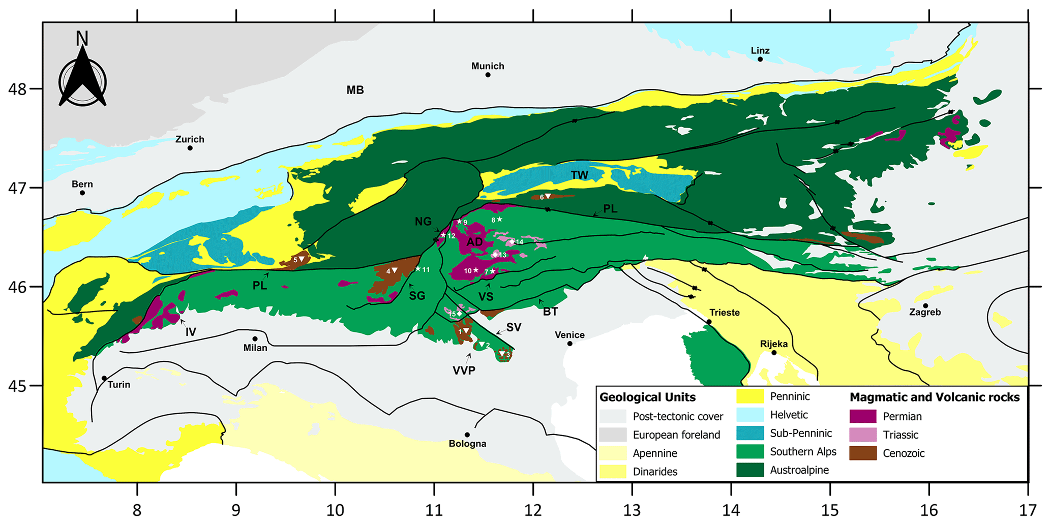
Figure 1 Geologic chart of the Alps, modified after Pfiffner (2015), and the main magmatic and volcanic bodies (Bigi et al., 1990a, b; Schuster and Stüwe, 2008). VVP: Venetian Volcanic Province; SV: Schio–Vicenza fault; BT: Bassano–Montello thrusts; VS: Valsugana thrust; SG: South Giudicarie Fault; NG: North Giudicarie Fault; AD: Athesian Volcanic District; PL: Periadriatic Line; IV: Ivrea–Verbano Complex; TW: Tauern Window; MB: Molasse Basin. (1) Lessini Mountains; (2) Berici Hills; (3) Euganei Hills; (4) Adamello batholith; (5) Masino–Bregaglia batholith; (6) Vedrette di Ries–Riesen Ferner batholith; (7) Cima d'Asta intrusion; (8) Bressanone–Chiusa intrusions; (9) Ivigna intrusion; (10) Monte Croce intrusion; (11) Monte Sabion intrusion; (12) Monte Luco intrusion; (13) Predazzo intrusion; (14) Monzoni intrusion; (15) Recoaro–Pasubio intrusions.

Our 3D density modeling comprises the entire central and eastern Alpine arc, and it extends down to a depth of 200 km, the same depth of the seismic tomography model. The conversion from seismic velocity to density is done with differentiated approaches, depending on the depth and position in the upper crust, lower crust or mantle. We used the most recent terrestrial- and satellite-derived gravity model and applied the global correction for terrain, which leads to very different Bouguer gravity values compared to the classic local correction up to the 167 km Hayford radius, but it is more realistic. The global fields require special attention because of the far-field effect of topography, and we included a dedicated section (Sect. 3.2), which explains how to deal with this problem, in order to use the fields in the regional density modeling. The Alpine gravity field has been modeled before (Ebbing et al., 2006; Spooner et al., 2019); novel in our study is the use of the Bouguer field corrected for the global topography. A recent study (Spooner et al., 2019) used an approach in which density is constant for lateral crustal domains with typical extension of 80 to 150 km, and the lithosphere is defined in layers of constant density. The layers have been defined with one layer each for unconsolidated and consolidated sediments, two layers for crystalline crust, one layer for subcrustal lithosphere, and one constant layer for the asthenosphere. In our approach, we have not posed any restrictions on the density variability, since we took full advantage of the high-resolution seismic tomography model, and emphasis was put on converting the seismic velocities to densities.

We addressed the central question of whether an alteration of the density structure or distribution in the crust and upper mantle below the extended Venetian magmatic Alpine province and the older Athesian magmatism (Bellieni et al., 2010) can be detected. In fact, during magmatic emplacement it can be expected that part of the molten crust is trapped in the lower crust. Only a portion (less than 10 wt %) of all molten rocks has erupted to the surface, and less than 60 wt % of the whole melt can be emplaced as intrusions in the upper crust (Angelo De Min, personal communication, 2019). Moreover, this crustal melting is often related to the emplacement of basic mantle-derived magma at the Moho discontinuity (magmatic underplating), which provides the necessary temperature to induce crustal melting.

The working hypothesis is that the above-mentioned gravity high could be related to the different magmatic events that have affected the study area at different times and to the consequent crustal densification and/or juvenile crust formation in underplating.

2 Geological introduction

The study area comprises most of the Alpine arc, with particular focus on the magmatism of the southern Alps (Fig. 1). The southern Alpine domain represents the undeformed retro-wedge of an orogeny of double vergence (Dal Piaz et al., 2003; Zanchetta et al., 2012). To the north, it is delimited by the dextral Periadriatic Line, also known as the Insubric Line. The Southalpine terrains formed the passive margin of the Gondwana Paleozoic shelf (Stampfli and Borel, 2002; Muttoni et al., 2009). The central Southalpine realms are characterized by three principal fault systems: the Valsugana fault, the Giudicarie fault and the Schio–Vicenza fault, all presumed to have been active since the late Permian (Viganò et al., 2013).

The late Paleozoic–Mesozoic rifting created a system of N–S-oriented faults, which induced the separation of the Lombardian Basin from the Veneto platform, as documented by the variable thickness of the Triassic and Cretaceous sediments (Bertotti et al., 1993). From the late Cretaceous to the early Eocene, the extensional regime was inverted due to the convergence between Gondwana and Laurasia, which generated contractional systems that initiated to the west of the Giudicarie and later extended to the eastern Dolomites (Zanchetta et al., 2012). Later, the Giudicarie line was affected by two contractional phases: in the middle to late Miocene the ENE–WSW-oriented thrusts of the Valsugana line developed, which exhumed part of the Hercynian basement. In the late Miocene and Pliocene the NE–SW-oriented thrusts of Bassano and Grappa–Montello developed, together with reactivation of faults in the Giudicarie (Castellarin and Cantelli, 2000; Castellarin et al., 2006). From the end of the Paleozoic up to the Tertiary different magmatic events affected the Southalpine realm with intrusive and effusive products that range from basic to acidic. According to Castellarin and Cantelli (2000), the volcanic and magmatic volumes contributed to considerably increasing the strength of the crust, with implications for the tectonics and geodynamics.

2.1 Permian magmatism

The Southalpine units were affected by large volumes of magmatism in the Paleozoic (285–260 Ma), with volcanic and plutonic products of acidic and basic type (Rottura et al., 1998). The thickness of the deposits has an average value of 900 m and reaches up to 2000 m (Rottura et al., 1998); they are represented by ignimbrites and rare flows of the Athesian Volcanic District. These volcanic rocks are bordered by several outcropping granitic intrusions, and the whole setting has some similarities to the coeval Ivrea–Verbano system (Angelo De Min, personal communication, 2019), which has been interpreted as the remnants of a super-volcano (Quick et al., 2009). The units that belong to this age are the porphyric Athesian platform and intrusions of Cima D'Asta, Bressanone–Chiusa, Ivigna, Monte Croce, Monte Sabion and Monte Luco. These magmatic products indicate important crustal contamination that could have been triggered by previous subduction (Variscan?), as indicated by their geochemical properties (Rottura et al., 1998). The magmatism probably originated in a post-Hercynian phase in a trans-tensive tectonic regime. According to Rottura et al. (1998) the magmatism was generated due to a lithospheric thinning followed by

• an asthenospheric upwelling,

• consequent partial melting of the asthenospheric mantle due to adiabatic decompression,

• production of gabbro, which, stored in underplating, has thermally perturbed the fertile crust, and

• consequent production of crustal melts that mixed with more evolved mantle-derived magma.

2.2 Triassic magmatism

The Triassic magmatism affected a continental area that at the time bordered the western paleo-Tethys and comprised the Southalpine, Dinaric, Transdanubian and Austroalpine domains (Abbas et al., 2018). In the Dolomites, the magmatic rocks are rare pyroclastics, dykes, sills, subaerial and marine volcanic, next to intrusions found at Predazzo and at Monti Monzoni. The origin of the magmatism has been hypothesized as due to plume, subduction or extensional events at lithospheric scale (Abbas et al., 2018; Casetta et al., 2018). The magmatism could be associated with the activation of regional strike-slip faults during the Ladinian (Abbas et al., 2018). In comparison with the Paleozoic magmatic event, the Triassic magmatic volume appears to be more modest and characterized by a stronger abundance of basic and intermediate products. In the Dolomitic area, these intrusions and vulcanites outcrop exactly inside the Permian magmatic structure. According to De Min et al. (2020) this could be related to the presence, at that time, of a depleted crust (depleted during the Paleozoic event) that scarcely interacted with the mantle-derived melts stored in underplating. These latter could therefore have evolved without heavily contributing to a crustal fusion. Smaller outcrops of this event are also present along the Valsugana valley and the Recoaro–Pasubio area.

2.3 Tertiary magmatism

From the late Paleocene to Oligocene, during 25 Myr, the terrains south of the Trento platform were affected by volcanism that extended over an area of 2000 km² (Milani et al., 1999). The principal units form the Lessini Mountains as well as the Berici and the Euganei Hills. The province is characterized by basalts, basanites, transitional basalts and trachytes, which are divided into three categories according to the chemical composition that ranges from alkaline to tholeiitic. The volcanic activity coeval with the formation of a (retro-)foreland basin is connected to a WNW–SSE contraction originating from the Adria–Europe convergence during the Alpine orogeny (Zampieri, 1995; Milani et al., 1999; Macera et al., 2008). During this same period, the calc–alkaline intrusives of Adamello and Masino–Bregaglia to the west of the southern Giudicarie were emplaced. These batholiths are composed of several intrusive units that formed during the Eocene in an interval between 31 and 35 Ma. Some Rb $/$ Sr datings estimate up to 42 Ma for the location Corno Alto (Martin and Macera, 2014).

3 Geophysical data

3.1 Seismic tomography database

The seismic tomography database from Kästle et al. (2018) was the starting point for the 3D density modeling. This recent model uses seismic stations distributed over the entire Alpine arc, with some stations in parts of central Europe and many stations in Italy. The tomography of Kästle et al. (2018) analyses surface waves generated by earthquakes with periods between 8 and 250 s and ambient noise observations in a period range of 4 to 60 s. Given the sensitivity of the seismic periods, the surface waves resolve the deep structures, and the ambient noise records the crustal structure and sedimentary basins, with an overlap of the two records for periods between 10 and 35 s. The tomography inversion included the global dataset of phase-velocity measurements of Ekström (2011), which were used to constrain the long-period velocity field. The checkerboard test showed that the Alps and Italy are well resolved, except for the French territory and the Adriatic and Tyrrhenian seas. The Dinarides and Pannonian basin belong to areas with lower resolution. Some problems also exist in the resolution of superficial structures in the eastern Po Basin due to scarce availability of seismic stations. The model resolves the upper mantle well in the Alpine foreland of the Adriatic Plate, central Europe, the Pannonian basin and the Ligurian Sea, with reduced resolution below the Alpine region. The model reports shear (V_s) velocities with a grid spacing in latitude of 0.1^∘, in longitude of 0.146^∘, and a vertical grid interval of 100 m for the upper 600 m, 500 m between 1 and 2.5 km, 1 km between 3 and 12 km, 2 km between 14 and 84 km, and 5 km between 85 and 200 km. The present study selects a portion of the model limited to longitudes 8–14^∘ and latitudes 43–49^∘.

3.2 Gravity field and topographic reduction

The gravity data were calculated from the global gravity model EIGEN6c4 (European Improved Gravity model of the Earth by new techniques; Förste et al., 2014b). The model combines observations from different geodetic satellites, such as LAGEOS-1/2 SLR, GRACE GPS-SST and GOCE, and it incorporates existing models from terrestrial data for the high-frequency part. It uses the Technical University of Denmark (DTU) ${\mathrm{2}}^{\prime }\times {\mathrm{2}}^{\prime }$ global gravity anomaly grid from satellite altimetry (Andersen, 2010; Andersen et al., 2010) over the oceans and the EGM2008 model (Pavlis et al., 2012) over the continents. The model is parameterized in terms of a table of spherical harmonic coefficients complete up to degree and order 2190. For degrees above N=235 in continental areas, the model reproduces the field of EGM08, and over oceanic areas the model is DTU12. The choice of the upper degree is justified by the fact that the creators of the model consider this maximum degree adequate, and statistical evaluations have been made up to this degree (Förste et al., 2014a).

It is customary to reduce the gravity field for the gravity effect of topography, which is available in terms of spherical harmonic expansion in the models of Hirt et al. (2016) and Hirt and Rexer (2015). The layers describing the topography have been divided into glaciers, oceans, lakes and solid crust, with their respective homogeneous densities equal to 917, 100, 1030 and 2670 kg m⁻³. We have used the particular model dv_ELL_RET2014PLUSGRS80, which includes the gravity of the ellipsoid. We refer to Rexer et al. (2016) for details on how the model was obtained.

Since several options exist for how to define the functional of the gravity value from the spherical harmonic models of the Earth's gravity and the topographic effect, we briefly give the fundamental definitions here. Further details can be found, for instance, in the textbooks Torge (2011), Torge and Müller (2012), and Barthelmes (2013).

The Bouguer anomaly is defined as

$$\begin{array}{}\text{(1)}& g_{\text{bg}}=g_{\text{fa}}-g^{\mathrm{T}}.\end{array}$$

Here the gravity effect of the topography (g^T) is subtracted from the free-air anomaly (g_fa). The free-air anomaly according to Molodensky (Torge, 2011) is defined as

$$\begin{array}{}\text{(2)}& \mathrm{\Delta }{g}_{\text{fa}}=g\left(P\right)-\mathit{\gamma }\left(Q\right),\end{array}$$

with g(P) being the observed value in point P, and γ(Q) is the gravity value of the reference ellipsoid calculated at the height of the telluroid. The gravity disturbance is defined as

$$\begin{array}{}\text{(3)}& \mathit{\delta }{g}_{\text{fa}}=g\left(P\right)-\mathit{\gamma }\left(P\right).\end{array}$$

Here the gravity field of the ellipsoid is subtracted from the observed gravity field, both calculated in the observation point P. The gravity anomaly and gravity disturbance are related to the disturbing potential T ($T\left(P\right)=W\left(P\right)-U\left(Q\right)$) as follows:

$$\begin{array}{}\text{(4)}& \mathit{\delta }{g}_{\text{fa}}\approx -{\displaystyle \frac{\partial (W-U)}{\partial h}},\end{array}$$

$$\begin{array}{}\text{(5)}& \mathrm{\Delta }{g}_{\text{fa}}\approx \mathit{\delta }{g}_{\text{fa}}-\mathrm{2}{h}^{-\mathrm{1}}(W-U).\end{array}$$

Here W is the Earth's gravity potential, U is the potential of the ellipsoid and h is the geometric height. Vaníček et al. (2004) show that due to the second term, which enters the definition of the gravity anomaly, the gravity disturbance must be used when deriving the gravity potential of the topography for the Bouguer correction. Otherwise, the second term in Eq. (5) would be applied twice. In the spectral domain the derivatives translate to the following:

$$\begin{array}{ll}\text{(6)}& {\displaystyle }\mathrm{\Delta }{g}_{\text{fa}}\left(r,\mathit{\lambda },\mathit{\phi }\right)& {\displaystyle }={\displaystyle \frac{GM}{r^{\mathrm{2}}}}+\sum _{n=\mathrm{0}}^N{\left({\displaystyle \frac{R}{r}}\right)}^n\left(n-\mathrm{1}\right){\displaystyle }& {\displaystyle }\cdot \sum _{m=\mathrm{0}}^n\left(C_{nm}^{\mathrm{T}}\cos m\mathit{\lambda }+S_{nm}^{\mathrm{T}}\sin m\mathit{\lambda }\right)\\ {\displaystyle }& {\displaystyle }\cdot P_{mn}\left(\sin \mathit{\phi }\right),\end{array}$$

$$\begin{array}{ll}\text{(7)}& {\displaystyle }\mathit{\delta }{g}_{\text{fa}}\left(r,\mathit{\lambda },\mathit{\phi }\right)& {\displaystyle }={\displaystyle \frac{GM}{r^{\mathrm{2}}}}+\sum _{n=\mathrm{0}}^N{\left({\displaystyle \frac{R}{r}}\right)}^n\left(n+\mathrm{1}\right){\displaystyle }& {\displaystyle }\cdot \sum _{m=\mathrm{0}}^n\left(C_{nm}^{\mathrm{T}}\cos m\mathit{\lambda }+S_{nm}^{\mathrm{T}}\sin m\mathit{\lambda }\right)\\ {\displaystyle }& {\displaystyle }\cdot P_{mn}\left(\sin \mathit{\phi }\right),\end{array}$$

where $C_{nm}^{\mathrm{T}}$ and $S_{nm}^{\mathrm{T}}$ are the Stokes coefficients of the gravity potential of either the Earth or topography, from which the Stokes coefficients of the ellipsoid have been subtracted. G is the gravitational constant, M is the Earth's mass, n and m are the degree and order of the spherical harmonic expansion, N is the maximum degree of the expansion, and r, λ and φ are the three spherical coordinates radius, longitude and latitude. The calculated gravity anomaly and disturbance are shown in Fig. 2, and it is seen that the gravity disturbance is systematically higher than the gravity anomaly, confirming Vaníček et al. (2004).

Figure 2 (a) Gravity anomaly and (b) gravity disturbance; both functionals have been calculated with the gravity model EIGEN6c4 (Förste et al., 2014b) using maximum degree N=2190 and calculation height h=5000 m.

Subtracting the gravity effect of topography g^T calculated with the model RET2014 (Rexer et al., 2016) as shown in Fig. 3b from the gravity disturbance derived from EIGEN6c4, the Bouguer gravity disturbance (Tenzer et al., 2019; Fig. 3c) is obtained. This Bouguer field corresponds to the classical complete Bouguer anomaly, which includes the topographic correction on top of the Bouguer plate correction, with the difference that we consider the entire Earth and do not limit the topographic corrections to the Hayford radius of 167 km. We achieved all calculations (Barthelmes, 2013) with the publicly available gravity calculation service of the ICGEM (International Center for Global Gravity Field Models; http://icgem.gfz-potsdam.de/home (last access: 5 February 2021). The 3D density modeling we intended to achieve was done on a window of less than 6^∘ latitude by 6^∘ in longitude and a maximum depth of 200 km. The limit in lateral and depth extension of the model produces a band-limited gravity field that can be modeled. It is therefore necessary to reduce the lowest degrees of the gravity field of topography, since they introduce a field that is due to distant masses and is uncorrelated with the regional properties of the gravity field that was modeled in the present study. We found that starting with degree and order N>10, the field of topography starts resembling the regional topography, and we used this value as a lower limit for the spherical harmonic expansion of the fields. This value agrees with the findings of Steinberger et al. (2010), who define degree 10 as the limit of lithospheric contributions due to lower degrees having their origin in the deep mantle or lower. The non-band-limited Bouguer field (Fig. 3a), the non-band-limited effect of topography (Fig. 3b) and the band-limited Bouguer field (Fig. 3c) are displayed in the respective maps. The band-limited Bouguer map (Fig. 3c) obtained for degrees $\mathrm{10}<N\le \mathrm{2190}$ (EIGEN 6c4 and RET2014) has the same features as the non-band-limited map (Fig. 3a), with the difference that now the bounds of the Bouguer anomalies are more similar to those of the regional topographic reduction obtained with the Hayford radius (e.g., Ebbing et al., 2006; Zanolla et al., 2006; Braitenberg et al., 2013; Spooner et al., 2019). In fact, the band-limited Bouguer disturbance is −160 mGal below the Alps and −130 mGal below the Apennines compared to the non-band-limited Bouguer values of −60 mGal over the Alpine arc. Another area with clear negative values is close to the front of the Tuscan–Emilian Apennines, presumably due to the combined effect of sediments from the Po Plain and the crustal thickening due to stacking of sediment layers in the Apennines. The markedly different values obtained with the global reduction are inherent to the distant masses that are neglected in the regional reduction but that are largely compensated for by the isostatic crustal thickness variations (Szwillus et al., 2016). In the following, we used the band-limited Bouguer disturbances (Fig. 3c).

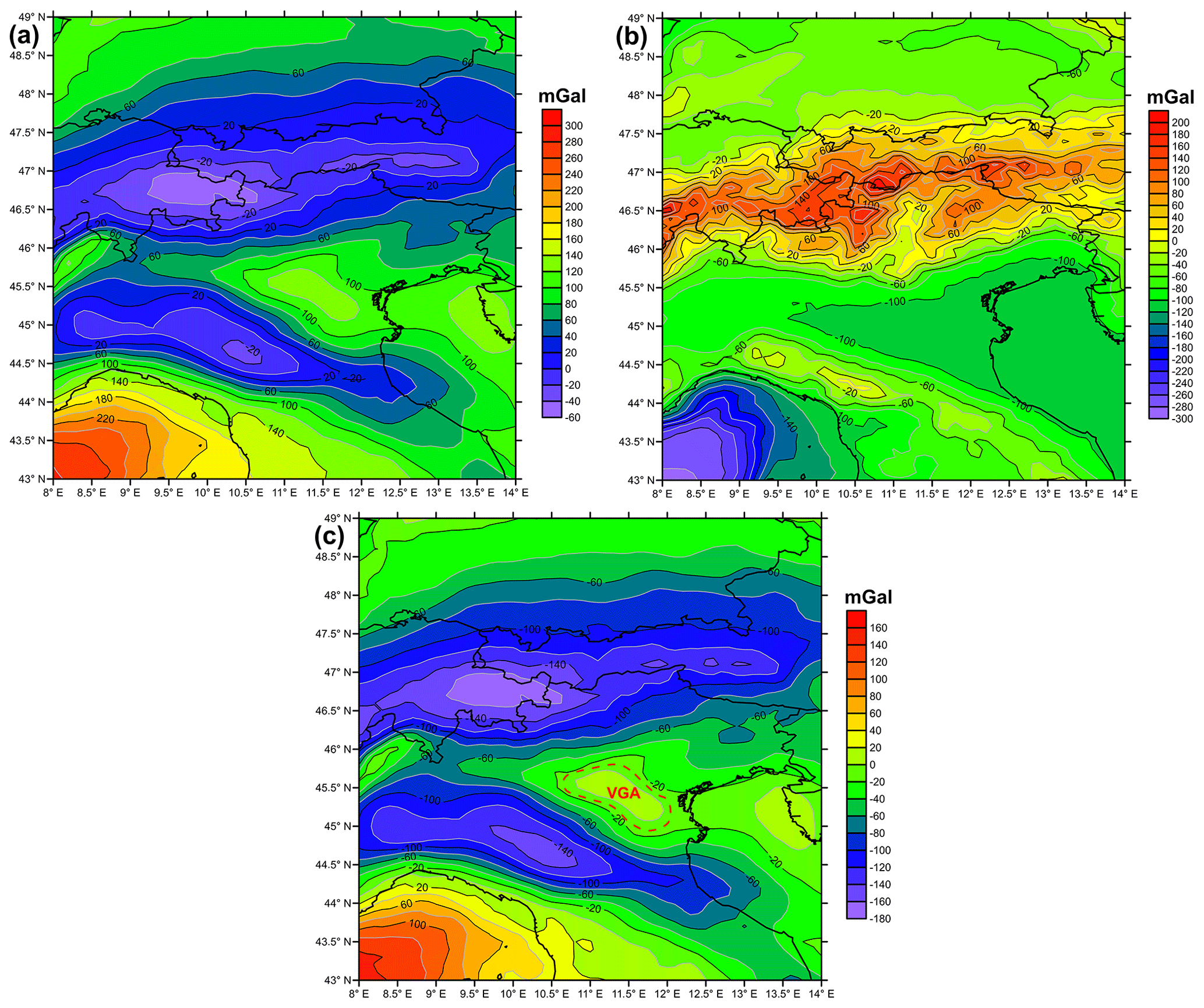
Figure 3 (a) Bouguer gravity disturbance using the gravity model EIGEN6c4 corrected with the topography model RET2014 (N=2190 and calculation height h=5000 m). (b) Gravity disturbance of the model RET2014 (Rexer et al., 2016) (with N=2190 and calculation height h=5000 m). (c) Band-limited Bouguer gravity disturbance using the gravity model EIGEN6c4 corrected with the topography model RET2014 (both calculated with $\mathrm{10}<N\le \mathrm{2190}$ and calculation height h=5000 m). VGA: Venetian Gravity Anomaly.

4 Method

The aim of this work was to develop a three-dimensional density model of the Alpine region constrained by seismic tomography. The method was developed in four steps:

• Moho discontinuity investigation;

• seismic wave velocity-to-density conversion for mantle and crustal layers;

• gravimetric forward modeling and comparison between modeled results and the observed gravity data; and

• inversion of the gravimetric residual and model density correction.

4.1 Moho discontinuity depth definition

The Moho discontinuity depth was defined by studying the vertical variation of the tomographic seismic velocity from Kästle et al. (2018). First of all, a preliminary velocity field analysis was conducted using other Moho models proposed by (a) Tesauro et al. (2008; EuCrust07), (b) Laske et al. (2013; Crust1.0) and (c) Grad et al. (2009; MohoGrad). From this field analysis, we discovered that the mean S-wave velocity of the crust–mantle transition is 4.1 km s⁻¹ with a standard deviation of 0.2 km s⁻¹ (Table 1). This velocity value is in agreement with the velocity change at Moho between 3.85 and 4.48 km s⁻¹ proposed in the 1D global model AK135 (Kennett et al., 1995). Therefore, based on this statistic, a preliminary result was obtained by researching the maximum vertical gradient of the velocity profile within a velocity range between 3.8 and 4.4 km s⁻¹, which represents the mean value plus and minus 1 standard deviation. To improve the stability and the reliability of this approach, another condition was imposed on the velocity surrounding the Moho surface obtained from the maximum gradient analysis. The S-wave velocity reported 4 km above and below the Moho surface had to be respectively smaller and larger than the typical velocity of the lower crust and uppermost mantle. The mean P-wave velocity of the European lower crust was estimated to be about 6.5 km s⁻¹, while in the upper mantle, the P-wave velocity of peridotite was larger than 8 km s⁻¹ (Christensen and Mooney, 1995). From this observation, the limits for the P-wave velocity above and below the Moho have been assigned values of 6.8 and 7.4 km s⁻¹.

Table 1 Statistics for the S-wave velocity (km s⁻¹) of the tomographic model (Kästle et al., 2018) at the depths of the Moho defined in three Moho models (Grad et al., 2009, MohoGrad; Tesauro et al., 2008, EuCrust07; Laske et al., 2013, Crust1.0). Average value ($V_{s_{\text{mean}}}$), minimum value ($V_{s_{\text{min}}}$), maximum value ($V_{s_{\text{max}}}$), and σ (standard deviation; km s⁻¹).

The results show good agreement with the Moho models proposed by other authors (Fig. 4). Some differences are represented by an important crustal thickening located in the Ivrea–Verbano (D1) area and below the Istrian region (D2). Also, the geometry and the depth found for the two main orogens (D3) are significantly different from the reference models, and our model seems to have a better resolution.

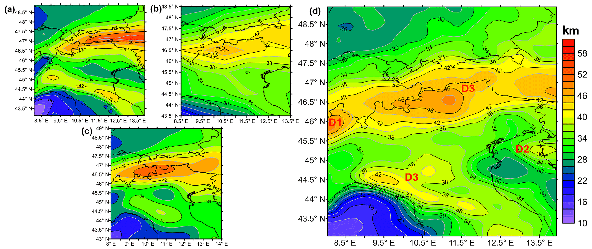
Figure 4 Map of the Moho depth according to (a) EuCrust07 (Tesauro et al., 2008), (b) CRUST1.0 (Laske et al., 2013), (c) MohoGrad (Grad et al., 2009) and (d) MohoTad (this work).

4.2 Seismic wave velocity-to-density conversion for mantle and crustal layers

The Moho discontinuity allowed us to divide the entire tomographic volume into crustal and mantle layers. For each layer, a different approach and relations were used to define the density values starting from the tomographic seismic velocity.

4.2.1 Crustal conversion

A huge set of relations have been proposed by different authors to convert the seismic wave velocity to density (Brocher, 2005), and most of these equations principally transform the compressional wave velocity (V_p) to density. For this reason, it was necessary to convert the tomographic V_s in V_p through the Brocher regression fit (Brocher, 2005), a relation obtained from seismic, borehole and laboratory data for different kinds of lithology valid for V_s between 0 and 4.5 km s⁻¹. Given the extreme variability of the crustal rocks present in the study area, a density estimation was carried out through two equations: “Gardner's rule” by Gardner et al. (1974) and a linear regression fit proposed by Christensen and Mooney (1995). The first is an empirically derived equation that relates seismic P-wave velocity to the bulk density of the lithology. It is very popular in petroleum exploration because it can provide information about the sedimentary lithology from interval velocities obtained from seismic data. On the other hand, Christensen and Mooney (1995) proposed a widely used linear density–V_p relation for crystalline rocks obtained from seismic refraction and laboratory data in order to define the continental crust features as a function of the different geodynamic context. In our work, the sedimentary rock velocity domain was distinguished from the crystalline domain by the velocity value at which the two curves intersect, as seen in Fig. 5 and also in Brocher (2005). For the sedimentary rocks, Gardner's rule was used, and for the crystalline rocks the linear fits of Christensen and Mooney (1995) were used, which are given for depth ranges from 10 to 50 km. The intersection velocity is dependent on depth; for the shallower depths of 10 km, for instance, the velocity is V_p=6 km s⁻¹, and at 50 km the intersection is at V_p=5.2 km s⁻¹ (see Fig. 5). The red symbols in Fig. 5 show the distribution of the final density values on the graph and will be discussed later. A mistake in the calculation of the density is made when the fit of Christensen and Mooney is used for sedimentary rocks and Gardner's rule is applied for crystalline rocks. This miscalculation is limited, however, if we analyze the velocities of sedimentary rocks and crystalline rocks. Due to the steeper slope of the relation of Christensen and Mooney, the resulting density is higher compared to Gardner's rule at the same velocity. For sedimentary rocks limited to the upper crust, the only rock that would have an overestimated density would be dolomite, since the other sedimentary rocks generally have a velocity below 6 km s⁻¹. For crystalline rocks, there is a limited number of rocks that have a velocity below 6 km s⁻¹ and are in danger of their density being overestimated by switching to Gardner's curve. For instance, only quartzites, andesites, meta-grauwacke and serpentinites are in danger of being misplaced (Mooney, 2007).

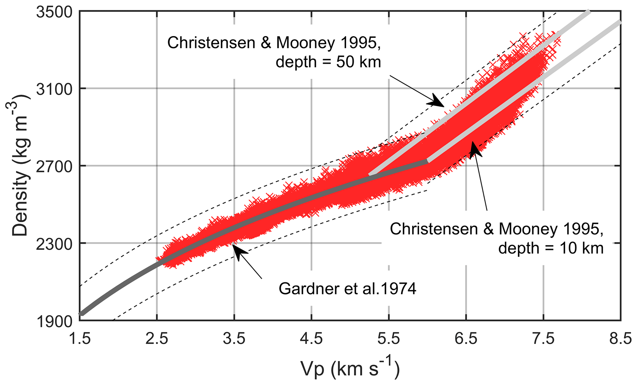
Figure 5 Comparison of published densities versus V_p relations discussed in Brocher (2005). The dark grey continuous line represents Gardner's equation, and the light grey continuous line represents the Christensen and Mooney (1995) linear regression fit. The relation of Christensen and Mooney (1995) has been published for different depth ranges from 10 to 50 km, and we show the two extreme relations. The stippled curves delimit the upper and lower bounds derived from the root mean square experimental scatter from the lines. The switch from Gardner's equation to the relation of Christensen and Mooney is made at the intersection of the two relations. The red symbols show the final distribution of the density versus velocity values of our final model at the end of the iterations.

4.2.2 Mantle conversion

A different approach was used for the velocity conversion in the uppermost mantle; in this case, the tomographic velocity model was compared to a synthetic upper mantle (SUM) model. The SUM was modeled with the open-source software Perple_X (Connolly, 2005), which allows the computation and mapping of the phase equilibria, rheological properties and density.

For this modeling the TECTON bulk rock composition model (Griffin et al., 2009) of the mantle was used, which represents an estimate of the mean composition of a Neoproterozoic–Phanerozoic subcontinental lithospheric mantle (SCLM), gained from xenolith suites and peridotite massif data. In Table A1, the major elements of the TECTON composition are shown; we used the most abundant elements up to a total content of 98.9 %, leaving out the minor elements with percentages less than 1 %. The software calculates the stable phases for a two-dimensional grid of the temperature (T) and pressure (P) conditions typical for the mantle up to a depth of 200 km ($T_{min}=\mathrm{350}{}^{\circ }\mathrm{C}$ to $T_{max}=\mathrm{1600}{}^{\circ }\mathrm{C}$, $P_{min}=\mathrm{0.1}\mathrm{GPa}$ to $P_{max}=\mathrm{7}\mathrm{GPa}$). The software requires setting some calculation parameters, which are defined here. The thermodynamic model is the Holland and Powell (1998) model, which is the default. For the computation of the phase equilibria and the elastic properties, the default parameters were used. Further options included no presence of saturated fluids, calculation with saturated components not present, chemical potentials, and activities and fugacities as non-independent variables. The adopted mineral phases for the SUM are olivine, clinopyroxenes, orthopyroxenes, garnet, spinel and plagioclase, and the thermodynamic model for these solid solutions is again the Holland and Powell (1998) database. We refer to the documentation of the software and the original paper for the thermodynamic modeling details, which are out of the scope of the present work.

The result consists of the equilibrium phase diagram, which shows the fields of stability of different equilibrium mineral assemblages for the adopted bulk rock composition depending on the P–T combinations. For each assemblage several parameters are given as well, from which we select V_s and density, as shown in Fig. 6.

Figure 6 Density and V_s plots of the model SUM as functions of pressure and temperature.

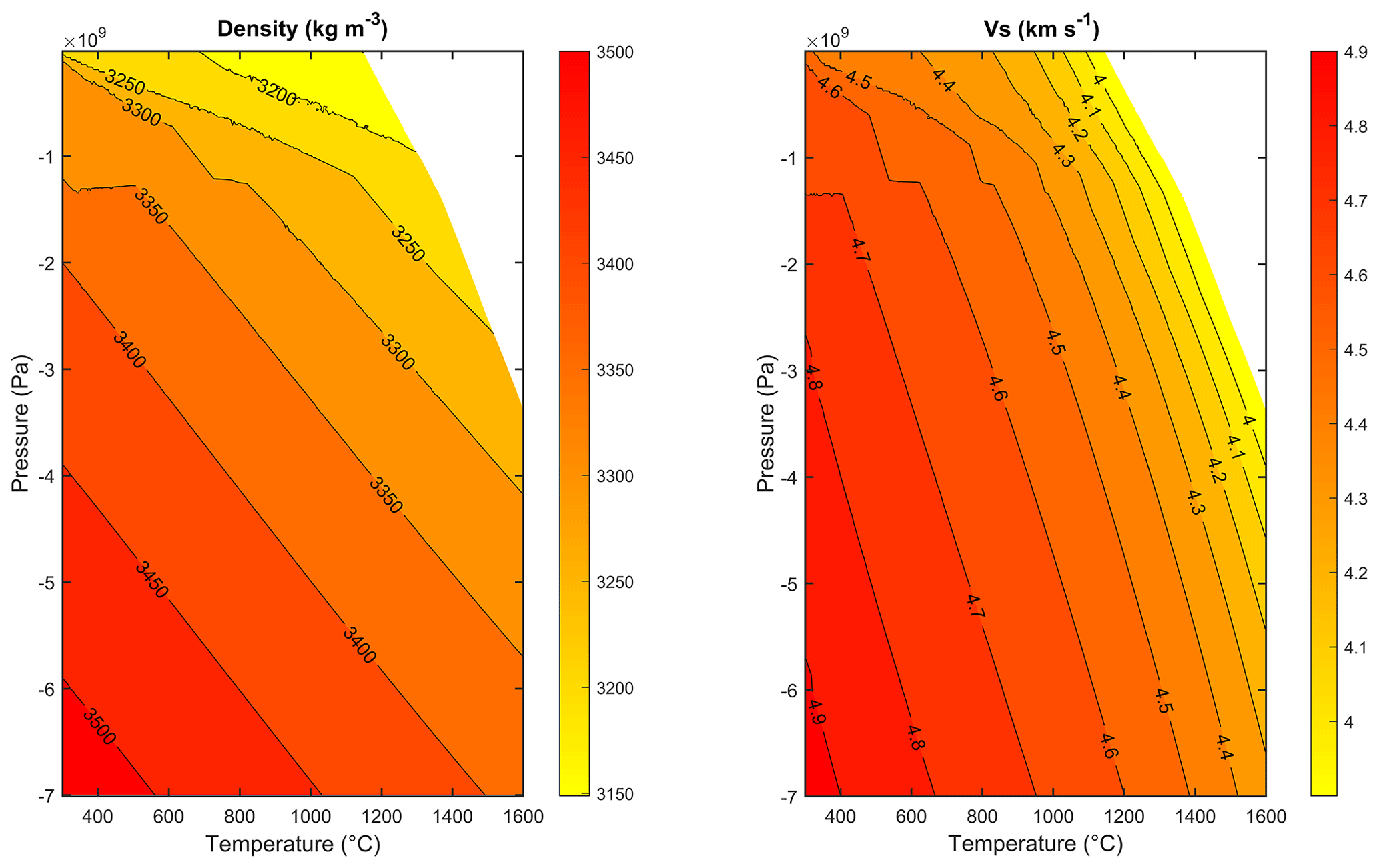
The conversion of the seismic velocity to density was made by comparing the tomographic velocity at its given depth with the synthetic velocity at the pressure corresponding to the depth. The pressure was calculated by integrating the lithospheric density column from the top to the corresponding depth. From the topography to the bottom of the crust, the crustal density model calculated from the crustal seismic velocities was used. The resulting pressure at the base of the crust was used to convert the seismic velocity to density in the resolution cell below the Moho and then iteratively downwards to the base of the model. The temperature was left unconstrained and corresponds to the value that allows matching the tomographic and synthetic velocity at the given pressure. The above-described density values define the starting model, which is corrected through the gravity inversion discussed in the next sections.

4.3 Gravimetric forward modeling and comparison between modeled results and the observed gravity data

In the previous section the transformation of P-wave velocities to density values was described. The next step was to discretize the entire model with tesseroids, which are mass elements defined in spherical geocentric coordinates (Anderson, 1976; Heck and Seitz, 2007; Wild-Pfeiffer, 2008; Grombein et al., 2013). This task was done by building these elements as a function of the original three-dimensional tomographic grid, from which we defined the density value of the tesseroids. In order to make the modeled gravity effect comparable with the observed gravity anomaly, the obtained density model was reduced by the reference density model PREM (Preliminary Reference Earth Model). This reference model represents the mean physical features of the Earth, including elastic parameters, seismic attenuation, density, pressure and the Earth-radius-dependent gravitational value as a function of radius. Being a global model, it was modified in order to obtain a dimensional model comparable with a continental crust by eliminating the first 3 km of seawater and lowering the Moho depth. All changes to the original PREM were done to maintain the pressure value at the base of the model as constant, and we call this modified model co-PREM (Fig. A1 in the Appendix). Applying co-PREM is equivalent to subtracting a constant value from the modeled gravity values, since gravity has a linear relation to density. For the crustal model, a different choice of the reference model will not alter the results because the constant gravity value will be absorbed in the mantle gravity residual field. Therefore, it could induce some effect on the density variations in the mantle. Assuming a difference in the gravity field of the reference model of 10 or 50 mGal, there would be an upward bias in the mantle densities of about 8 or 40 kg m⁻³, a very small value compared with mantle densities of close to 3400 kg m⁻³.

Figure 7a shows the result of the gravitational forward modeling developed through the software Tesseroids (Uieda et al., 2016). The gravity anomaly map presents two well-defined negative anomalies induced by the crustal thickening below the orogens and the extensive positive anomaly produced by the Tyrrhenian crust. At large scale, the modeled anomaly reproduces in broad outline the observed data (Fig. 3c), and from the difference between observed and modeled anomalies, we obtained the residual gravity map (Fig. 7b). The residual map shows that the modeled anomaly differs from the observed map by values that range from −40 to +220 mGal. Furthermore, the residual outlines three regions characterized by different trends: Germany and part of Switzerland are characterized by negative values reaching peaks around −40 mGal (A1), and the Tyrrhenian basin shows a positive residual around +80 mGal (A2), while the residuals are generally positive in all of the remaining study areas, reaching values of +200 mGal (A3).

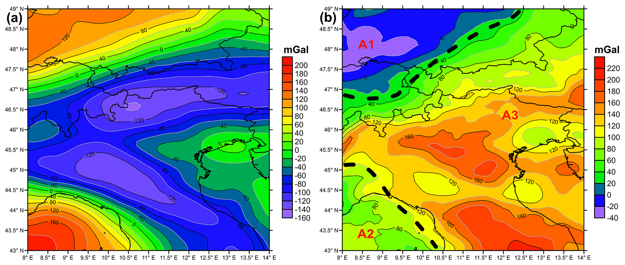
Figure 7 (a) Gravity anomaly map from the forward modeling. (b) Residual gravity map obtained from the difference between the Bouguer gravity disturbance (with $\mathrm{10}<N\le \mathrm{2190}$) and the forward gravity anomaly map. A1: Germany and Switzerland negative residual region; A2: positive residual region of Tyrrhenian basin; A3: Adriatic and Alpine domain characterized by high residual. The black dashed lines divide the three different regions.

4.4 Inversion of the gravimetric residual and model density correction

Theoretically, the gravity residual map represents the extent to which the starting density model diverges from one of the infinite number of possible density distributions that produced the measured gravity anomaly. In order to improve the reliability of the starting density model an inversion algorithm was developed based on the residual between observed and modeled data. As seen in Fig. 8, the first step is to separate the long-wavelength residual component from the short wavelengths and to estimate the different contributions of the mass sources that generate the residual signal.

Figure 8 Flowchart of the linear inversion algorithm.

The distinction between the mantle and crustal contribution, which corresponds to the long and short wavelengths, respectively, has been made by fitting a third-order polynomial surface to the values of the residual map (Fig. 9). The choice of the order was made through a qualitative evaluation depending on the features and the large-scale trend in the residual anomaly map.

Figure 9 (a) Mantle residual component map (long wavelengths). (b) Crustal residual component maps (short wavelengths).

Starting with degree zero up to degree 3, the long-wavelength signal is uncorrelated with topography and geology, and it was assigned to the mantle component. Starting with degrees higher than 3 the polynomial started to show smaller-scale features that correlated with the geometrical and physical properties of the crust. We therefore think that the third-order polynomial is qualitatively the correct choice to separate the mantle from the crustal component. The mantle component has a long-period trend oriented NW–SE. The third-order polynomial allows separating this very long-wavelength signal from the crustal contribution. Considering the changes in absolute gravity values, we observe that after subtracting the first model obtained from the seismic data, the values had been reduced from a range of 360 mGal to 270 mGal (Fig. 7). The biggest large-scale anomalies had been largely reduced, leaving a residual field that is dominated by smaller-scale gravity anomalies. Separating the mantle contribution from the crustal contribution shows that the high amplitude of the residual comes from the mantle (Fig. 9a), with a range value of 270 mGal, whereas the crustal contribution is mostly limited to a range value of 140 mGal (Fig. 9b), with small-scale features reaching a range value of 190 mGal.

Then, once we obtained the two components, we apply an iterative algorithm, in which a rough first density correction was computed with the “infinite slabs gravimetric effect” equation:

$$\begin{array}{}\text{(8)}& \mathrm{\Delta }\mathit{\rho }={\displaystyle \frac{\mathrm{\Delta }g}{\mathrm{2}\mathit{\pi }GH}},\end{array}$$

where Δρ is the density correction, Δg is the short or long gravimetric residual component, H represents the thickness of the considered layer (crustal or mantle layer), and G is the gravitational constant. Then the density correction was applied to the starting density model, and the vertical distribution of the total mass correction was assigned through the following equation:

$$\begin{array}{}\text{(9)}& {\mathit{\rho }}_{i_{\text{new}}}\left(z\right)={\mathit{\rho }}_{i_{\text{old}}}\left(z\right)+\mathrm{\Delta }{\mathit{\rho }}_n{H}_n\left({\displaystyle \frac{{\mathit{\rho }}_{i_{\text{old}}}\left(z\right)}{{\sum }_{i=\mathrm{1}}^N{\mathit{\rho }}_{i_{\text{old}}}\left(z\right)\mathrm{\Delta }{z}_i}}\right),\end{array}$$

where ${\mathit{\rho }}_{i_{\text{new}}}$ and ${\mathit{\rho }}_{i_{\text{old}}}$ are respectively the new and the old density values, Δρ_n is the density correction, H_n is the height of the considered layer (crust or mantle layer), and Δz_i represents the height of the mass element belonging to the single density profile. We applied the density correction, obtained a new mass distribution and computed the forward modeling of the corrected density model in the next step. The results of the latter operation were compared with the observed data, producing for each iteration a new gravimetric residual map. The density was free to vary at the stage of the iterations inside the bounds of acceptable densities in the crust and mantle, defined from laboratory measurements. These are as follows: density in the crust, 2200 to 3000 kg m⁻³; mantle, 3000 to 3500 kg m⁻³. The iteration was stopped when the root mean square residual reached a value below 3 mGal. The number of iterations needed was six for the crust and five for the mantle. This algorithm allowed us to define the density correction, which was applied to the three-dimensional starting model and allowed us to compare the gravity effect of this new mass distribution with the observed data. The root mean square density correction over the volume of crust and mantle and the root mean square decrease in the gravity residual during iterations are shown in Fig. 10. It can be seen how the gravity residual quickly decays in the first iterations and then remains close to constant when reaching the level of 3 mGal. The final density values in relation to the V_p velocity are shown in Fig. 5 as red symbols. It can be seen that the final density values are inside the root mean square experimental deviations from the theoretical relations between density and velocity, and they are therefore physically acceptable. The map of the final total crustal density corrections, corresponding to the sum of the corrections calculated in each of the six iterations and the final gravity residual, are displayed in Fig. 11a and b.

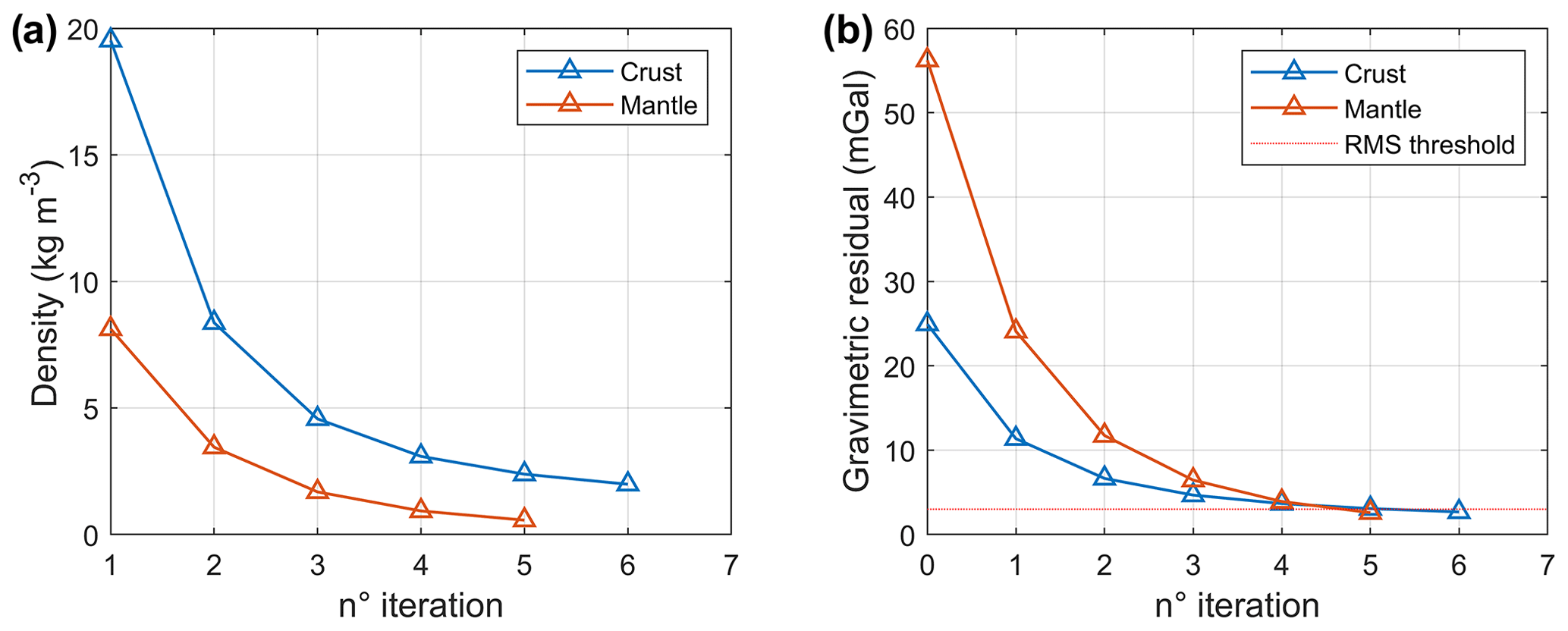
Figure 10 Illustration of the effectiveness of the iteration steps in the crust and mantle. (a) Root mean square density correction over the volume of the crust and mantle during iterations. (b) Root mean square decrease in the gravity residual, separated for the signal of the crust and mantle during iterations. The iterations were stopped when a root mean square residual of 3 mGal was reached.

Figure 11 (a) Final gravity residual after crustal inversion, (b) sum of density corrections obtained during crustal inversion and (c) root mean square value of the density uncertainty along the crustal column after the final correction.

Several error sources intrinsically affect the final 3D density model. A forward error propagation is very difficult to perform because quantitative estimates of all errors starting from the seismic model are not available to us. Therefore, it is hard to provide a quantitative error estimation of the final density model. However, some general aspects can be considered to understand what the main sources of uncertainty and their effects are during the modeling process. First of all, the Moho discontinuity definition has a larger impact for the middle to long component of the gravimetric field, and uncertainty in some kilometers of this surface can produce several milligals (mGal) of gravity variation, significantly changing the modeled anomaly. Analyzing the proposed method, another set of critical error sources includes the different equations used for the P-wave velocity–density transformation. The proposed equation reflected regional studies based on different input data acquired from different geological contexts. Other error sources are the uncertainties affecting the tomographic velocity model used as input data for this study and the linear inversion algorithm based on the simple Bouguer plate correction. Apart from the mentioned uncertainties, we estimate the amount of correction on the crustal density model after the final iteration of the inversion and use this as a quantification of the uncertainty. For the crustal column, we obtain a root mean square value of the final correction of up to 2 kg m⁻³, as shown in Fig. 11c. The final gravity residual has a root mean square value of less than 2.7 mGal.

5 Results

5.1 Alpine region density distribution

Figure 12 shows horizontal slices of the final density model at increasing depths ranging between 5 and 40 km. Here we describe the main features.

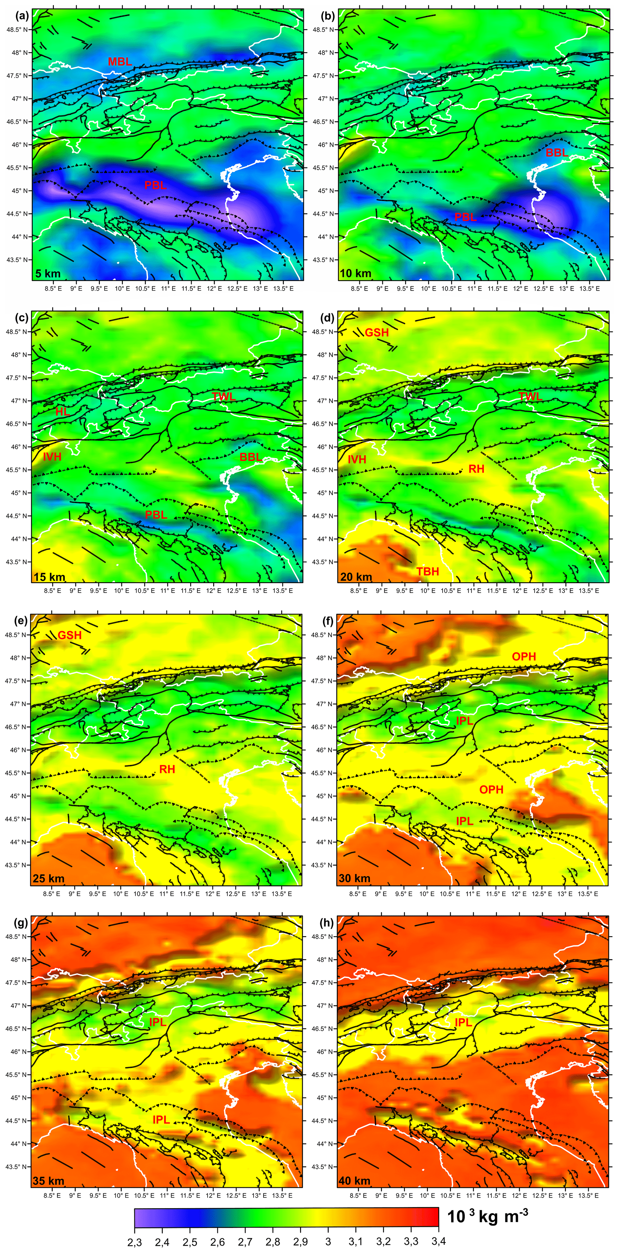
Figure 12 Slice of the density model at (a) 5 km, (b) 10 km, (c) 15 km, (d) 20 km, (e) 25 km, (f) 30 km, (g) 35 km and (h) 40 km. MBL: low density of Molasse Basin; PBL: low density of Po Basin; BBL: low density of Belluno Basin; HL: low density of Helvetic nappe; TWL: low density of Tauern Window; IVH: high density of Ivrea–Verbano; GSH: high density of Rhine graben system; RH: high-density ridge; TBH: high density of Tyrrhenian basin; IPL: low density of orogen inner part; OPH: high density of orogen outer part.

In the first kilometers up to 15 km of depth (Fig. 12a–c), the low density values are due to the two main sedimentary basins situated in the foredeeps of the Alps and Apennines. On the European Plate, the Molasse Basin is trending in the W–E direction along the northern Alps front (LMB), and this sedimentary layer is wider and thinner in the western part, whilst it becomes more elongated and thickens in the eastern Bavarian part. On the Adriatic Plate, the Po Basin (PBL) is characterized by a thicker and less dense sedimentary layer than in the Molasse Basin. The Molasse Basin is shallower (average thickness 5 km, maximum thickness 9 km) than the Po Basin (average thickness 9 km, maximum thickness 13 km). As shown in Fig. 12a and b, both modeled basins show a progressive decrease in the densities towards the eastern part of the sedimentary layer (especially at the south of the Po River mouth).

Remaining in the first 15 km, a homogenous density region (2650–2750 kg m⁻³) features the Alpine orogenic upper crust. Inside this domain a relatively low-density anomaly (2650 kg m⁻³) corresponding to the Helvetic nappe (HL) and the Tauern Window (TWL) is present, while in the Ivrea–Verbano (IVH) zone the density reaches the typical values of the lower crust (2850–2900 kg m⁻³).

Between 15 and 20 km (Fig. 12c and d) the modeled density represents the gradual transition from the upper to lower crust, except in the Tyrrhenian basin (TBH), where the high density values indicate the crust–mantle transition, in agreement with the Moho depths in Fig 4d. In this depth interval, the Adriatic crust is denser than the European crust; furthermore, a W–E-trending high-density ridge (RH) (2900 kg m⁻³) follows the western Southalpine domains, passing near the Schio–Vicenza fault up to the buried front of the Apennines. As previously seen in the first kilometers, a relatively low-density domain remains below the Helvetic terrain (HL) and the Tauern Window (TWL). A further lower-density patch is present in the Adriatic Sea, below the northern Apennines (PBL) and facing the Valsugana thrust system (BBL).

Figure 12e and f show the lower crustal modeled density of the European and Adriatic plates, where the relatively low density values characterizing the lower crust of the inner part of the Alpine and Apennine orogens (2800–2850 kg m⁻³) are visible (IPL), while in the outer parts of the two orogens and in the foredeep regions (OPH), the average density is higher (2900–2950 kg m⁻³). Very high values affect the lower crust of the northwestern part of the study area close to the upper Rhine graben system (GSH); furthermore, the W–E-trending high-density ridge is still present (RH), reaching higher values at this depth (up to 3000 kg m⁻³ below the Giudicarie and Schio–Vicenza fault system). At 30 km of depth, mantle density is present on the northern European Plate and below the Adriatic Sea, in agreement with the Moho depths in Fig. 4d.

At greater depth (Fig. 12g and h), the modeled density features of the Alps and Apennines crustal roots and the inner part (LIP) of the two belts are characterized by densities lower (2800–2850 kg m⁻³) than the surroundings. Below the orogen's crustal roots, the mantle is marked by a density average value of around 3300 kg m⁻³.

We have also computed the weighted average density for the crustal layer (Fig. 13). The average density distribution reproduces and synthesizes all the features seen above. On the European Plate, different domains are present for the area close to the upper Rhine graben (GSH) (high density of 2860–2900 kg m⁻³) and the Molasse Basin (MBL) (2740–2800 kg m⁻³). Also, the Alps show a density zonation in good agreement with the surface geology: the Helvetic terrain (HL) and Tauern Window (TWL) are on average less dense than the Penninic (PH), Austroalpine (AH) and Southalpine (SH) nappes. The Adriatic domain is represented by a highly complex density distribution with a heterogeneous low-density area highlighting the Po Basin (PBL), the adjacent Adriatic, and other two more restricted areas situated in the Piedmont (PDL) and Belluno Basin(BBL) regions. In the Apennines, the density values follow the main structural lines defined by the stack of NE-to-E-verging thrust fronts and the back-arc basin affected by extensional tectonics. In the Southalpine domain, the model generally shows high density values, especially in the Ivrea–Verbano Complex (IVH) (3000 kg m⁻³) and at the Valsugana thrust system (SH) (2870 kg m⁻³) in the eastern part. The previously discussed W–E high-density ridge that develops from the Ivrea–Verbano anomaly to the Schio–Vicenza fault system (RH), which also affects the Trento platform, is additionally seen in the average crustal density map.

Figure 13 Average density map. MBL: low density of Molasse Basin; PBL: low density of Po Basin; BBL: low density of Belluno Basin; PDL: low density of Piedmont Basin; HL: low density of Helvetic nappe; PH: high density of Penninic nappe; AH: high density of Austroalpine nappe; TWL: low density of Tauern Window; IVH: high density of Ivrea–Verbano; GSH: high density of Rhine graben system; RH: high-density ridge; SH: high density of Southalpine domains.

5.2 Modeled density in the Venetian Gravity Anomaly area

Three representative transects across the main gravity anomaly structures of the central and eastern southern Alps are illustrated in Fig. 14 and discussed in the following.

Figure 14 Sections across the 3D density model for illustration. The positions of the profiles are shown in (a) and (b). (a) Band-limited Bouguer gravity disturbance map. (b) Crustal average density map. (c) Section A oriented NW–SE centered on the Vicenza–Verona gravity high. (d) Section B oriented SW–NE centered on the gravity high. (e) Section C oriented WNW–SSE centered on the gravity high. MB1: first mushroom-shaped body with high density; MB2: second mushroom-shaped body; PB: Po Basin; VVP: Venetian Volcanic Province; SGF: South Giudicarie Fault; AB: Adamello batholith; PL: Periadriatic Line; VTF: Valsugana Thrust Front; ATF: Apennine Thrust Front; RH: high-density ridge; IVH: high-density anomaly of Ivrea–Verbano; BB: Belluno Basin; TP: Trento platform; LB: Lombardian Basin.

The A section (Fig. 14) shows the density distribution along the main direction of the Venetian Gravity Anomaly parallel to the Schio–Vicenza fault. The low density in the southern part of the profile represents the sediment layer that reaches a thickness of around 13 km in the deepest part (longitude 12.5^∘ E in the profile). As seen before, between the South Giudicarie Fault (SGF) and the buried Apennine Thrust Front, there is again an increased density area (RH) situated between 25 km and the Moho discontinuity extending between 10.8 and 11.8^∘ E, with a density of 2900–3000 kg m⁻³. This increased density in the lower crust can be recognized, for instance, by an upward shift of the 2900 kg m⁻³ isoline, distancing it from the Moho. In the middle crust, two limited mushroom-shaped bodies are lying between 10 and 25 km; the first (MB1) is located below the Venetian Volcanic Province (VVP) and above the high-density plateau (RH) close to latitude 11.5^∘ N, while the second (MB2) is situated below an area between the South Giudicarie Fault (SGF) and the Periadriatic Line (PL), corresponding to the outcropping Adamello batholith (AB). Although outside our focus area, we mention a density high along profile A, which is located NW of the Periadriatic Line (PL) and affects depths of 10 to 30 km. Along profile A it is approximately located at longitude 9.8^∘. The recent work of Rosenberg and Kissling (2013) interprets the crustal velocity variations and highlights the upwelling of the velocity lines north of the Periadriatic Line, with a lower effect in the central Alps and an increase in the effect towards the central western Alps. They interpret it as lower crustal accreted terrain, which is deformed and brought to upper crustal levels north of the Periadriatic Line. From our modeling, this unit not only has high velocity, but also increased density.

The NE–SW-oriented section (Fig. 14 – B section) is orthogonal to the well-developed sedimentary wedge of the Alpine and Apennines foredeep (PB), which is 10 km thick in the deepest part and has density values between 2350 and 2550 kg m⁻³. Using the 2700 kg m⁻³ contour line as a marker for the top of the Mesozoic carbonate platform, it is possible to note that the contour line depth increases between latitude 46^∘ N and latitude 44^∘ N. The 2700 kg m⁻³ contour line reaches the surface in front of the Valsugana thrust system (at around 46^∘ N latitude) (Fantoni and Franciosi, 2010). North of the Valsugana Thrust Front (VTF), corresponding to the southern Alpine belt, the model shows density values of 2750 kg m⁻³ for the upper crust and 2800 up to 2900 kg m⁻³ for the middle to lower crust. In the central part of the section the model reports a very high-density plateau (RH) situated in the lower crust that develops from the buried Apennine Thrust Front (ATF) up to the outcropping south-vergent thrust (VTF).

The last section (close to W–E) crosses the Ivrea–Verbano area (Fig. 14 – C section) and then runs along the Po sediment basin. Lateral density variations of the upper crust are well correlated with the different basin domains represented from west to east by the Lombardian Basin (LB), the Trento platform (TP) and the Belluno Basin (BB). The mid-crust already shows high density (e.g., greater than 2800 kg m⁻³) values at a depth of 20 km, and this value distribution corresponds to the previously discussed high-density ridge (RH) seen in the average density map (Fig. 14b).

6 Discussion

Several geophysical models have been developed for the Alpine lithosphere in the past, especially using seismic (Gebrande et al., 2006; Kästle et al., 2018) and gravity data as modeling constraints (Ebbing et al., 2006; Spooner et al., 2019). In this work, for the first time, a high-resolution three-dimensional seismic tomography model has been adopted as a starting model for the computation of a 3D density model using the algorithm discussed before. The results show a highly complex density distribution in good agreement with the different geological domains of the Alpine area represented by the European Plate, the Adriatic Plate and the Tyrrhenian basin. Notwithstanding the offsets that can occur between the outcropping geology and the intracrustal tectonic domains, we find that the average crustal density map correlates with the different tectonic realms. The Adriatic-derived terrains (Southalpine and Austroalpine) of the Alps are typically denser (2850 kg m⁻³), whilst the Alpine zone, composed of terrains of European provenance (Helvetic and Tauern Window), presents lower density values (2750 kg m⁻³). This density relation has also been noted by Spooner et al. (2019), indicating that this physical parameter could be used as a marker for the different tectonic domains.

The Southalpine and Austroalpine provinces were the locus of sporadic yet occasionally widespread magmatism. The magmatic occurrences are associated with strongly variable tectonic regimes, which range from clearly collision-related (the Austroalpine Paleogene plutonism; i.e., Vedrette di Ries (Rieserferner Group), Adamello, Masino–Bregaglia), to late or slightly post-orogenic associated with basin formations shortly after the main Variscan orogeny (Permian magmatism; e.g., Athesian volcanism and the Ivrea Verbano and Serie dei Laghi Group), to clearly post-orogenic (Triassic; e.g., the Predazzo–Monzoni complexes), and finally to an almost within-plate environment peripheral to the Alpine belt (the Oligocene Venetian Volcanic Province) (Bellieni et al., 2010).

These magmatic activities undoubtedly changed the thermal setting at the time and, after cooling, increased the crustal rigidity, especially in the Venetian Alps (Dolomites), which appear today to be the least deformed and shortened in the whole southern Alps domain (Castellarin et al., 2006).

In this domain south of the Dolomites, the well-known positive Bouguer gravity anomaly is present, located between the towns of Verona and Vicenza, which covers the Venetian Volcanic Province (VVP). The short-wavelength content of this gravity high can reasonably be explained by the presence of a shallow Mesozoic carbonate platform (Trento platform) and basement that hosted several volcanic bodies, as demonstrated by field evidence and the intra-sedimentary magnetic bodies proposed by Cassano et al. (1986) on the basis of magnetic and well data. According to this interpretation, the isolated mushroom-shaped body modeled in the middle to upper crust could be related to the Triassic and Cenozoic magmatic activity. These intrusions developed below the Venetian Volcanic Province and could correspond to the Predazzo–Monzoni Complex and the Adamello and Masino–Bregaglia plutons respectively emplaced in the Dolomites and westward of the South Giudicarie Fault. However, the remaining part of this signal corresponds to the signal generated by the lower crustal source component, which gives an origin to the long wavelength of the positive Bouguer anomaly, as also proposed by Zanolla et al. (2006). During the Permian, the Austroalpine and Southalpine units were affected by magmatism, high-temperature–low-pressure metamorphism (HT-LP) and extensional tectonics. Intra-continental basins hosting Permian volcanic products have been interpreted as developed either in a late collisional strike-slip or in a continental rifting setting (Spalla et al., 2014; Spiess et al., 2010, and references therein). Regarding the geodynamic context, all evidence suggests that this magmatic pulse was induced by post-Variscan lithospheric thinning that produced crust–mantle detachment and large ultramafic crustal underplating, together with the development of a Permian basin (Dal Piaz and Martin, 1998). For a fuller understanding of this process, we may refer to the modern model tested in the western southern Alps in the Ivrea–Verbano zone, where the entire crustal section of an underplated and metamorphosed Hercynian basement crops out, overlain by volcanic and sediment formations (Quick et al., 1995, 2009; Sinigoi et al., 2011). In the central southern Alps the Permian activity is represented by the porphyry plateau of the Bolzano province (Athesian plateau) and numerous granitic–granodioritic intrusions. Considering the large scale of this process, it is reasonable to suppose the scattered presence of mafic underplating in the whole Alpine realm, confirmed by the Permian–Triassic gabbro bodies and related HT-LP metamorphism emplaced in the Austroalpine and Southalpine continental crust (Spalla et al., 2014). According to this hypothesis, the high density values modeled for the Adriatic lower crust (high-density ridge, HR; Fig. 12d and f) are consistent with the densities of a basaltic mantle-derived rock; hence, this anomalous lower crust could be interpreted as mafic underplating emplaced between the crustal–mantle transition during Permo-Triassic post-collisional lithospheric extension.

Historically, the deep source of the Venetian (positive) Gravity Anomaly has been explained by a thinned crust of 25–27 km (Scarascia and Cassinis, 1997; Finetti, 2005; Cassinis, 2006; Gebrande et al., 2006). This approach has promoted the development of several Moho models of the Alps that invoke a relatively shallow mantle situated in the central southern Alps, especially for gravity-modeling-derived Moho models (Ebbing et al., 2001; Braitenberg et al., 2002). Recently, other seismic methodologies, such as local earthquake tomography, receiver functions and ambient noise tomography, have allowed researchers to develop 3D high-quality crustal models of the Alps (Kästle et al., 2018; Spada et al., 2013), and this family of Moho models points to a crustal thickness of 30–35 km in the Venetian (positive) Gravity Anomaly region, supporting the possibility that the gravimetric anomaly is related to an intracrustal denser source (mafic underplating). Also, Mueller and Talwani (1971), in their Alpine crustal model, proposed a high-density distribution for the Southalpine lower crust that connects the Venetian gravity high to the Ivrea–Verbano zone.

Unfortunately, the kinematics of magmatic underplating have been described mainly by petrophysical models explaining the genesis of the outcropping rocks, while the available geophysical images of underplated material remain relatively sparse and confined to specific tectonic environments (Thybo and Artemieva, 2013). Our work adds a geophysical model based on the gravity field to demonstrate the existence of underplating to an area related to an orogen. Underplating from a gravimetric analysis has also been postulated, for instance, in the context of the Paraná large igneous province (Mariani et al., 2013) and the western Siberian large igneous province (Braitenberg and Ebbing, 2009).

7 Conclusions

The aim of this work is to study the density distribution of the Alpine lithosphere, with the specific target of characterizing the sources of the well-known Venetian Gravity Anomaly high. A new approach based on three-dimensional seismic tomography as a starting model for the computation of a 3D density model has been developed. We propose an innovative approach that includes several numerical algorithms and that provides a Moho definition, a velocity–density conversion, gravimetrical forward modeling and finally a linear inversion based on a gravimetric residual map. The results for the Alpine structure highlight that all terrains of Adriatic provenance (Austroalpine and Southalpine) are denser (2850 kg m⁻³) than the European terrains (2750 kg m⁻³), suggesting that this physical parameter could be used as a marker to characterize the different tectonic domains involved in the Alpine regions (Spooner et al., 2019).

The studied gravity anomaly is located in the central Southalpine domain; this area is the locus of several magmatic and volcanic activities developed from the Carboniferous up to the Paleogene (Athesian Volcanic Province, Predazzo–Monzoni and Venetian Volcanic Province), which modified the rheological and thermal settings. The results of our density model suggest that the gravity anomaly sources could be related to the following:

• localized mushroom-shaped magmatic bodies intruded into the middle to upper crust, which could correspond to the Triassic and Cenozoic Predazzo–Monzoni, Masino–Bregaglia and Adamello plutons, now outcropping in the southern Alps; and

• mafic underplating was emplaced in the lower crust during the Permian lithosphere attenuation, similarly to the model developed for the Ivrea–Verbano Complex present in the western part of the southern Alps.

We also considered alternative source models for this gravity anomaly, based on which different authors postulate a stretched and thinned Adriatic crust located between the Giudicarie Thrust Front and the Schio–Vicenza fault, but today several Moho models of the Alps exist that refute this model.

The approach we use could represent a generally applicable method to achieve insights into large-scale crustal density distributions starting from seismic tomography, and it allowed us to carry out a high-resolution density model for the Alpine region. The expected improvement of more robust and high-resolution seismic tomography models, as well as the development of a non-linear inversion algorithm, could enhance the reliability of density models in the future.

Appendix A

Table A1 Median composition of the sublithospheric continental mantle (SLCM) normalized to 100 %, which was used for modeling the conversion of density to seismic velocity, dependent on temperature and pressure conditions (Griffin et al., 2009).

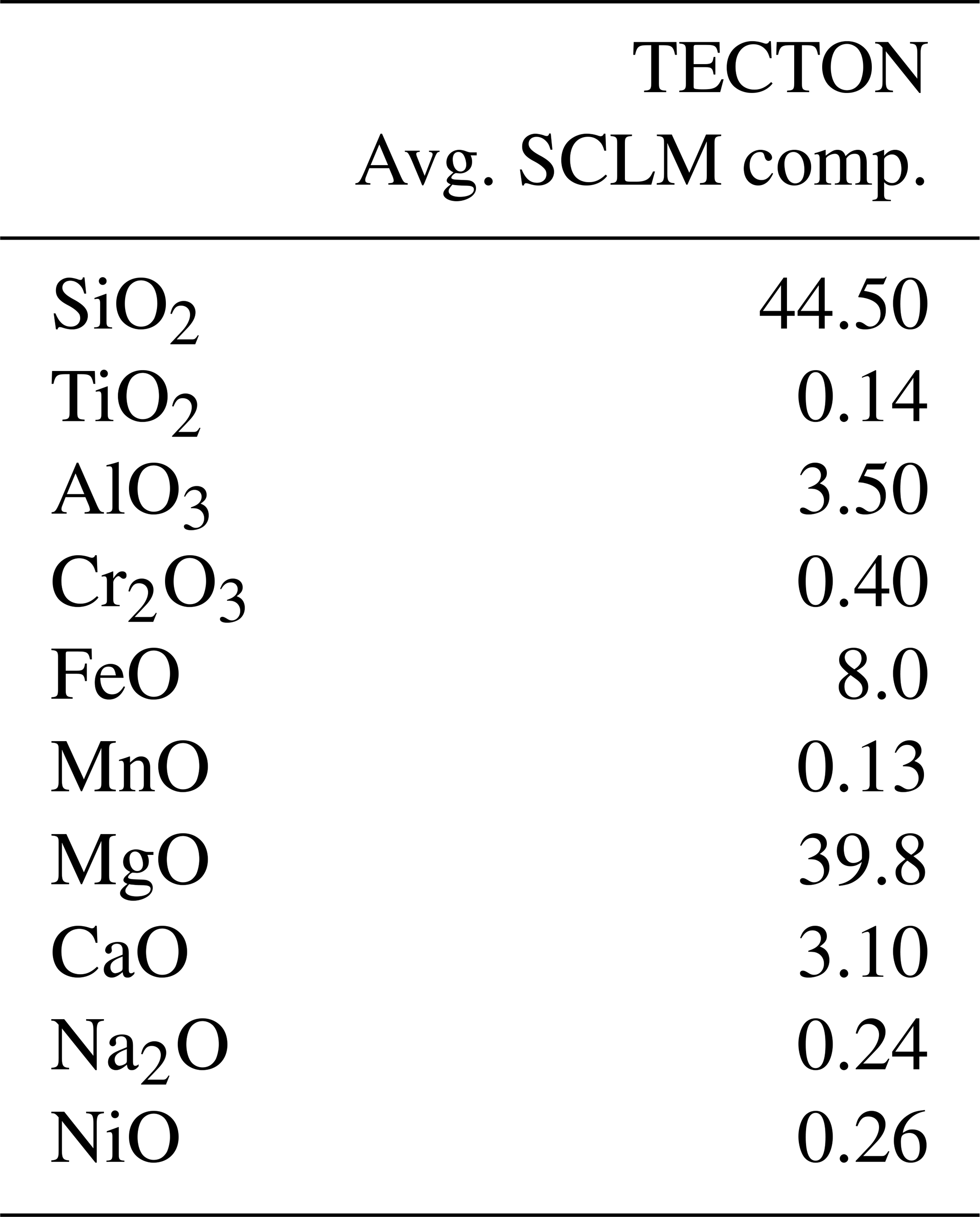
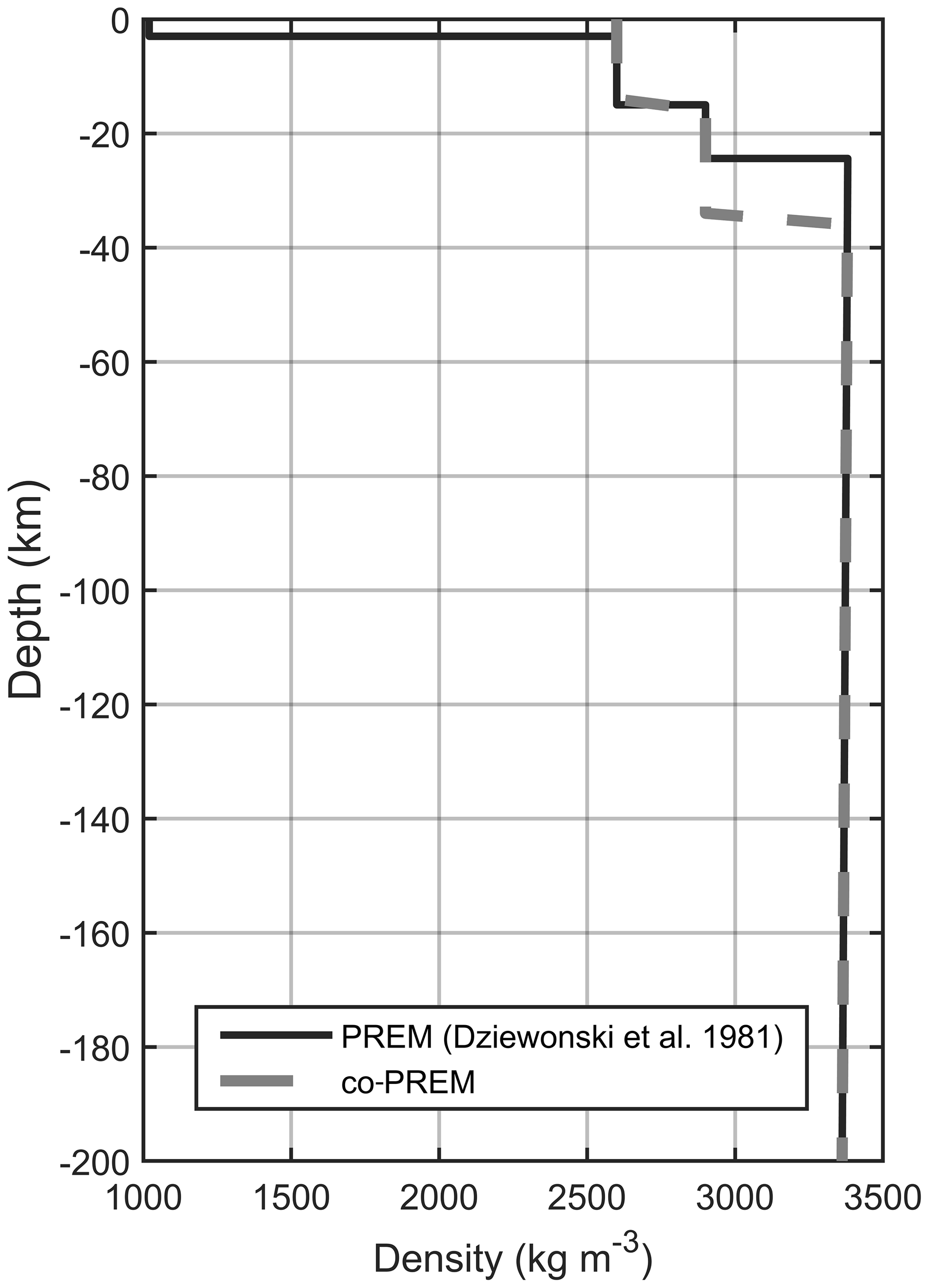
Figure A1 Density of PREM and the modified co-PREM used as a reference in the modeling procedure.