On the choice of finite element for applications in geodynamics

Geodynamical simulations over the past decades have widely been built on quadrilateral and hexahedral finite elements. For the discretization of the key Stokes equation describing slow, viscous flow, most codes use either the unstable Q₁×P₀ element, a stabilized version of the equal-order Q₁×Q₁ element, or more recently the stable Taylor–Hood element with continuous (Q₂×Q₁) or discontinuous ($Q_{\mathrm{2}}\times P_{-\mathrm{1}}$) pressure. However, it is not clear which of these choices is actually the best at accurately simulating “typical” geodynamic situations.

Herein, we provide a systematic comparison of all of these elements for the first time. We use a series of benchmarks that illuminate different aspects of the features we consider typical of mantle convection and geodynamical simulations. We will show in particular that the stabilized Q₁×Q₁ element has great difficulty producing accurate solutions for buoyancy-driven flows – the dominant forcing for mantle convection flow – and that the Q₁×P₀ element is too unstable and inaccurate in practice. As a consequence, we believe that the Q₂×Q₁ and $Q_{\mathrm{2}}\times P_{-\mathrm{1}}$ elements provide the most robust and reliable choice for geodynamical simulations, despite the greater complexity in their implementation and the substantially higher computational cost when solving linear systems.

1 Introduction

For the past several decades, the geodynamics community's workhorse for numerical simulations of the incompressible Stokes equations has been the use of (continuous) piecewise bilinear and/or trilinear velocity and piecewise constant (discontinuous) pressure finite elements, often in combination with the penalty method for the solution of the resulting linear systems (e.g., Donea and Huerta, 2003). This velocity–pressure pair is often referred to as the Q₁×P₀ Stokes element and sometimes as the Q₁×Q₀ element (Gresho and Sani, 2000). It is used, for example, in the ConMan (King et al., 1990), SOPALE (Fullsack, 1995), SLIM3D (Popov and Sobolev, 2008), CitcomCU (Moresi and Gurnis, 1996; Zhong, 2006), CitcomS (Zhong et al., 2000; McNamara and Zhong, 2004; Zhong et al., 2008), Ellipsis (Moresi et al., 2003; O'Neill et al., 2006), UnderWorld (Moresi et al., 2003), DOUAR (Braun et al., 2008), and FANTOM (Thieulot, 2011) codes and has therefore been used in hundreds of publications.

The popularity of this element can be explained by its very small memory footprint and ease of implementation and use. On the other hand, it has a rather low convergence order that makes it difficult to achieve high accuracy; maybe more importantly, the element is known not to satisfy the so-called Ladyzhenskaya–Babuška–Brezzi (LBB) condition condition (e.g., Donea and Huerta, 2003) and is therefore unstable. This instability noticeably manifests itself through oscillatory pressure modes (e.g., Fig. 18 of Thieulot et al., 2008 or Fig. 36 of Thieulot, 2014) and makes it not suited for large-scale three-dimensional simulations coupled to iterative solvers (May and Moresi, 2008). The unreliability of the pressure also makes this element a dubious choice for models in which some of the parameters – e.g., the density or the viscosity – depend on the pressure.

The more modern alternative to this choice is the Taylor–Hood element that uses (continuous) polynomials of degree k for the velocity and of degree k−1 for the pressure, where k≥2.¹ This element is not only LBB-stable, but owing to its higher polynomial degree is also convergent of higher order. It is therefore widely used in commercial flow solvers and is also the default element for the Aspect code in geodynamics (Kronbichler et al., 2012; Heister et al., 2017). This element is obviously more difficult to implement, and building efficient solvers and preconditioners is also more complicated (Kronbichler et al., 2012; Clevenger et al., 2020). However, these drawbacks can be mitigated by building on one of the widely available finite-element libraries that have appeared over the past 20 years; for example, Aspect inherits all of its finite-element functionality from the deal.II library (see Bangerth et al., 2007; Arndt et al., 2020). We will note that one can also use a number of variations of the underlying idea of the Taylor–Hood element, for example on quadrilaterals and hexahedra by using $Q_k\times P_{-(k-\mathrm{1})}$ (see, for instance, May et al., 2015, Lechmann et al., 2011, and Thielmann and Kaus, 2012) in which the pressure is discontinuous and of (total) polynomial degree k−1, but missing the part of the finite-element space on every cell that distinguishes the space Q_k on quadrilaterals and hexahedra from the space P_k that is typically used on triangles and tetrahedra.² Another variation is to enrich the pressure space by a constant shape function on each cell (see, for example, Boffi et al., 2011, and the references therein). All of these alternatives are stable for k≥2, and in keeping with common usage of the term, we will also refer to all of these variations as Taylor–Hood or Taylor–Hood-like elements even though they are strictly speaking not what Taylor and Hood proposed in Taylor and Hood (1973).

A third option is the use of Q₁×Q₁ elements with both velocity and pressure using bilinear or trilinear shape functions. This combination of elements is not LBB-stable by default, but numerous stabilization techniques – typically adding a pressure-dependent term to the mass conservation equation – have been proposed in the literature (see, e.g., Norburn and Silvester, 2001; Elman et al., 2014; Gresho et al., 1995). Herein, we will discuss in particular the variation by Dohrmann and Bochev (2004) that is simple to implement and does not involve any tunable parameter. This approach is used in the Rhea code (Burstedde et al., 2009, 2013) in conjunction with adaptive mesh refinement (AMR), allowing for the numerical solution of whole Earth models at high resolutions (Stadler et al., 2010; Alisic et al., 2012). Another example of the use of this method is the work of Leng and Zhong (2011), also using AMR, to study thermochemical mantle convection. Both the ELEFANT code with an application to the 3D thermal state of curved subduction zones (Plunder et al., 2018) and the GALE code (Moresi et al., 2012), with application to the 3D shapes of metamorphic core complexes (Le Pourhiet et al., 2012) or oceanic plateau subduction (Arrial and Billen, 2013), use the stabilized Q₁×Q₁ method. Finally the ADELI code was coupled to a stabilized Q₁×Q₁ flow solver in the context of lithosphere–asthenosphere interaction studies (Cerpa et al., 2014, 2015, 2018).

The availability of all of these options leads us to the main question of this paper: which element should one use in geodynamics computations based on the Stokes equations? Or, in the absence of clear-cut conclusions, which ones should not be used? On the face of it, this seems like a simple question: the consensus in the computational science community is that using moderately high-degree elements (say, k=3 or k=4) yields the best accuracy for a given computational effort (measured in CPU cycles) unless one wants to change the solver technology to use matrix-free methods whereby even higher polynomial degrees become more efficient. This conclusion is based on the higher convergence order of higher-degree methods but balanced by the rapidly growing cost of matrix assembly and linear solver effort for higher-degree methods. On the other hand, the recommendation to use higher-degree methods is predicated on the assumption that the solution is smooth enough – say, the velocity is in the Sobolev space H^k+1 of functions that have, loosely speaking, at least k+1 derivatives – that one can actually achieve a convergence rate of 𝒪(h^k) in the energy norm and 𝒪(h^k+1) in the L₂ norm, where h is the mesh size. This assumption generally requires that all coefficients, such as density and viscosity, are sufficiently smooth on length scales resolvable by the mesh. This may not be the case in realistic geodynamics problems given that density and viscosity often depend discontinuously on the solution variables (velocity or strain rate, pressure, temperature, and compositional variables); indeed, in many models, the viscosity may vary by orders of magnitude on short length scales.

Such considerations put into question whether higher-order methods are really worth the effort for actual geodynamics simulations. Given these divergent theoretical thoughts, the only way to resolve the question is by way of numerical comparisons. We have consequently extended Aspect so that it can use all of the element combinations above, and we will use these implementations in the comparisons in this paper.

Goals of this paper. Having outlined the conflict between the expected superiority of higher-degree elements for the Stokes equation on the one hand and the expected lack of smoothness of solutions in realistic geodynamic cases, our goals in the paper are as follows.

1. Quantitatively compare the solution accuracy of the various options (Q₁×P₀, $Q_k\times Q_{k-\mathrm{1}}$, $Q_k\times P_{-(k-\mathrm{1})}$ and stabilized Q₁×Q₁) using a variety of analytical benchmarks for which the exact solution is known. As we will see below, there is little point working with k>2 in geodynamics applications, and so the only cases we consider for Taylor–Hood-like elements are Q₂×Q₁ and $Q_{\mathrm{2}}\times P_{-\mathrm{1}}$.

2. Extend these numerical comparisons to cases in which it is known that the stabilized Q₁×Q₁ demonstrates problematic behavior that may make it unusable in many practical situations. In particular, we will consider the case of buoyancy-driven flows.

3. Conclude our considerations by comparing the available options using a realistic geodynamical application. This will allow us to draw conclusions as to what element one might want to recommend for geodynamics applications.

While we have approached this study with an open mind and without a strong prior idea of which element might be the best, let us end this Introduction by noting that members of the crustal dynamics and mantle convection communities have occasionally expressed a dislike of the stabilized Q₁×Q₁ element for its inability to deal with large lithostatic pressures and free surfaces absent special modifications of the formulation. For example, Arrial and Billen (2013) comment on the need to modify the physical description of the problem due to the stabilization (with references replaced by ones listed at the end of this paper).

All the models were run with the open source code Gale. […] Gale uses Q₁–Q₁ elements to describe the pressure and the velocity. However, this formulation is unstable and a slight compressible term is added in the divergence equation to stabilize it (Dohrmann and Bochev, 2004). Ideally, this term should be applied on the dynamic pressure and not on the full pressure. To fix this, a hydrostatic term corresponding to the reference density and temperature profile, is subtracted from the full pressure and the body force vector.

Few other negative comments concerning the Q₁×Q₁ element appear on record in the published literature, although one can find the following quote in Lehmann et al. (2015).

We do not consider the Q₁×Q₁/stab element (Dohrmann and Bochev, 2004; Bochev et al., 2006; Burstedde et al., 2009), as stabilization of this element is achieved by introducing an artificial compressibility that dominates for flows mainly driven by buoyancy variations (May et al., 2015). In geophysical flow models this yields unphysical pressure artifacts for cases where both the free surface of the Earth and mantle flow are considered, because the driving density contrast between cold sinking plates and the warmer surrounding Earth's mantle is much smaller than the density difference between rocks and air (Kaus et al., 2010; Popov and Sobolev, 2008; Mishin, 2011). In our experience, this results in artificial “compaction” of the Earth’s mantle if Q₁×Q₁/stab element is used, which makes them unsuitable for these purposes.

Indeed, our numerical experiments will encounter a similar issue; see Sect. 6.

We are not aware of any other significant publications in the geodynamics literature that specifically discuss the relative trade-offs between the elements we consider herein, specifically between the Q₁×P₀ and Taylor–Hood elements, and consequently believe that our discussions here are useful for the community.

2 The governing equations

For the purpose of this paper, we are concerned with the accurate numerical solution of the incompressible Stokes equations:

$$\begin{array}{}\text{(1)}& {\displaystyle }-\mathrm{\nabla }\cdot \left[\mathrm{2}\mathit{\eta }\mathit{\epsilon }\left(\mathit{u}\right)\right]+\mathrm{\nabla }p& {\displaystyle }=\mathit{\rho }\mathit{g}& {\displaystyle }\mathrm{in}\mathrm{\Omega },\text{(2)}& {\displaystyle }-\mathrm{\nabla }\cdot \mathit{u}& {\displaystyle }=\mathrm{0}& {\displaystyle }\mathrm{in}\mathrm{\Omega },\end{array}$$

where η is the viscosity, ρ the density, g the gravity vector, ε(⋅) denotes the symmetric gradient operator defined by $\mathit{\epsilon }\left(\mathit{u}\right)=\frac{\mathrm{1}}{\mathrm{2}}(\mathrm{\nabla }\mathit{u}+\mathrm{\nabla }{\mathit{u}}^T)$, and $\mathrm{\Omega }\subset {\mathbb{R}}^d,d=\mathrm{2}$ or 3 is the domain of interest. Both the viscosity η and the density ρ will, in general, be spatially variable; in applications, this is often through nonlinear dependencies on the strain rate ε(u) or the pressure, but the exact reasons for the spatial variability are not of importance to us here: what matters is that these coefficients may vary strongly and on short length scales.

In applications, the equations above will be augmented by appropriate boundary conditions and will be coupled to additional and often time-dependent equations, such as ones that describe the evolution of the temperature field or of the composition of rocks (see, for example, Schubert et al., 2001; Turcotte and Schubert, 2012). This coupling is also not of interest to us here.

3 Discretization using finite-element methods

3.1 Formulation and basic error estimates

For the comparisons we intend to make in this paper, Eqs. (1)–(2) are discretized using the finite-element method. A straightforward application of the Galerkin method yields the following finite-dimensional variational problem: find ${\mathit{u}}_h\in {\mathcal{U}}_h,p_h\in {\mathcal{P}}_h$ so that

$$\begin{array}{}\text{(3)}& \begin{array}{rl}\left(\mathit{\epsilon }\left({\mathit{v}}_h\right),\mathrm{2}\mathit{\eta }\mathit{\epsilon }\left({\mathit{u}}_h\right)\right)-(\mathrm{\nabla }\cdot {\mathit{v}}_h,p_h)& =({\mathit{v}}_h,\mathit{\rho }\mathit{g}),\\ -(q_h,\mathrm{\nabla }\cdot {\mathit{u}}_h)& =\mathrm{0},\end{array}\end{array}$$

for all test functions ${\mathit{v}}_h\in {\mathcal{U}}_h,q_h\in {\mathcal{P}}_h$. Here, $(a,b)={\int }_{\mathrm{\Omega }}a\left(\mathit{x}\right)b\left(\mathit{x}\right)\mathrm{d}x$. For simplicity, we have omitted terms introduced through the treatment of boundary conditions. The finite-dimensional, piecewise polynomial spaces 𝒰_h and P_h can be chosen in a variety of ways, as discussed in the Introduction. In particular, if they are chosen as 𝒰_h=Q_k and ${\mathcal{P}}_h=Q_{k-\mathrm{1}}$ – i.e., the Taylor–Hood element – then the discrete problem is known to satisfy the LBB condition and the solution is stable (Elman et al., 2014). Here, Q_s is the space of continuous functions that are obtained on each cell K of a mesh 𝕋 by mapping polynomials of degree at most s in each variable from the reference cell [0,1]^d. Likewise, the problem is stable if one chooses 𝒰_h=Q_k and ${\mathcal{P}}_h=P_{-(k-\mathrm{1})}$, where now P_−s is the space of discontinuous functions obtained by mapping polynomials of total degree at most s from the reference cell. In both of these cases, we expect from fundamental theorems of the finite-element method (see, for example, Elman et al., 2014) that the convergence rates are optimal, i.e., that the errors satisfy the relationships

$$\begin{array}{}\text{(4)}& {\displaystyle }\begin{array}{rl}\Vert \mathrm{\nabla }(\mathit{u}-{\mathit{u}}_h){\Vert }_{L_{\mathrm{2}}}& =\mathcal{O}\left(h^k\right),\\ \Vert \mathit{u}-{\mathit{u}}_h{\Vert }_{L_{\mathrm{2}}}& =\mathcal{O}\left(h^{k+\mathrm{1}}\right),\\ \Vert p-p_h{\Vert }_{L_{\mathrm{2}}}& =\mathcal{O}\left(h^k\right),\end{array}\end{array}$$

where h is the maximal diameter over all cells in the mesh 𝕋.

On the other hand, if one chooses 𝒰_h=Q₁ and 𝒫_h=P₀, i.e., the unstable Q₁×P₀ element with piecewise linear continuous velocities and piecewise constant discontinuous pressure, then the best convergence rates one can hope for would satisfy the following relationships based solely on interpolation error estimates:

$$\begin{array}{}\text{(5)}& {\displaystyle }\begin{array}{rl}\Vert \mathrm{\nabla }(\mathit{u}-{\mathit{u}}_h){\Vert }_{L_{\mathrm{2}}}& =\mathcal{O}\left(h\right),\\ \Vert \mathit{u}-{\mathit{u}}_h{\Vert }_{L_{\mathrm{2}}}& =\mathcal{O}\left(h^{\mathrm{2}}\right),\\ \Vert p-p_h{\Vert }_{L_{\mathrm{2}}}& =\mathcal{O}\left(h\right).\end{array}\end{array}$$

In practice, if the numerical solution shows pressure oscillations (see for instance Sani et al., 1981a, b), one will not even observe the rates shown above but might in fact obtain a worse pressure convergence rate, for example $\Vert p-p_h{\Vert }_{L_{\mathrm{2}}}=\mathcal{O}\left(h^{\mathrm{1}/\mathrm{2}}\right)$.

Finally, if one uses 𝒰_h=Q₁ and 𝒫_h=Q₁, then this unstable element combination can be made stable if one replaces the discrete formulation (3) by the following stabilized version due to Dohrmann and Bochev (2004):

$$\begin{array}{}\text{(6)}& \begin{array}{rl}\left(\mathit{\epsilon }\left({\mathit{v}}_h\right),\mathrm{2}\mathit{\eta }\mathit{\epsilon }\left({\mathit{u}}_h\right)\right)-(\mathrm{\nabla }\cdot {\mathit{v}}_h,p_h)& =({\mathit{v}}_h,\mathit{\rho }\mathit{g}),\\ (q_h,\mathrm{\nabla }\cdot {\mathit{u}}_h)-\left((I-{\mathit{\pi }}_{\mathrm{0}})q_h,{\displaystyle \frac{\mathrm{1}}{\mathit{\eta }}}(I-{\mathit{\pi }}_{\mathrm{0}})p_h\right)& =\mathrm{0}.\end{array}\end{array}$$

Here, I is the identity operator and π₀ is the projection onto piecewise constant functions – i.e., π₀f is the function that on each cell is equal to the mean value of f on that cell. For this element, the rates one might hope for are as follows (see again Dohrmann and Bochev, 2004):

$$\begin{array}{}\text{(7)}& {\displaystyle }\begin{array}{rl}\Vert \mathrm{\nabla }(\mathit{u}-{\mathit{u}}_h){\Vert }_{L_{\mathrm{2}}}& =\mathcal{O}\left(h\right),\\ \Vert \mathit{u}-{\mathit{u}}_h{\Vert }_{L_{\mathrm{2}}}& =\mathcal{O}\left(h^{\mathrm{2}}\right),\\ \Vert p-p_h{\Vert }_{L_{\mathrm{2}}}& =\mathcal{O}\left(h\right).\end{array}\end{array}$$

Dohrmann and Bochev (2004) report that for some test cases, one might in fact obtain $\Vert p-p_h{\Vert }_{L_{\mathrm{2}}}=\mathcal{O}\left(h^t\right)$ with t≈1.5, though it is not clear whether this rate can be obtained for all possible applications. We also observe this improved rate in one of our benchmarks in Sect. 5.

We end this section by noting that in many of the setups we use in Sect. 5, the boundary conditions we impose lead to a problem in which the pressure is only determined up to an additive constant. The same is then true for the linear system one has to solve after discretization. As a consequence, we can only meaningfully compute quantities such as $\Vert p-p_h{\Vert }_{L_{\mathrm{2}}}$ if both the exact and the numerical solution are normalized; a typical normalization is to ensure that their mean values are zero. Aspect enforces this normalization after solving the linear system.

3.2 A closer look at the error estimates

A comparison of Eq. (4) with Eqs. (5) and (7) would suggest that the Taylor–Hood element can obtain substantially better rates of convergence if one only chooses the polynomial degree k large enough.

However, this is an incomplete understanding because the 𝒪(h^m) notation hides the fact that the constants in this behavior depend on the solution. More specifically, a complete description of the error behavior would replace Eq. (4) by the following statement: there are constants $C_{\mathrm{1}},C_{\mathrm{2}},C_{\mathrm{3}}<\mathrm{\infty }$ so that

$$\begin{array}{}\text{(8)}& {\displaystyle }\begin{array}{rl}\Vert \mathrm{\nabla }(\mathit{u}-{\mathit{u}}_h){\Vert }_{L_{\mathrm{2}}}& \le C_{\mathrm{1}}{h}^k\Vert {\mathrm{\nabla }}^{k+\mathrm{1}}\mathit{u}{\Vert }_{L_{\mathrm{2}}},\\ \Vert \mathit{u}-{\mathit{u}}_h{\Vert }_{L_{\mathrm{2}}}& \le C_{\mathrm{2}}{h}^{k+\mathrm{1}}\Vert {\mathrm{\nabla }}^{k+\mathrm{1}}\mathit{u}{\Vert }_{L_{\mathrm{2}}},\\ \Vert p-p_h{\Vert }_{L_{\mathrm{2}}}& \le C_{\mathrm{3}}{h}^k\Vert {\mathrm{\nabla }}^{k}p{\Vert }_{L_{\mathrm{2}}}.\end{array}\end{array}$$

The validity of these statements clearly depends on the solution being regular enough so that ∇^k+1u and ∇^kp actually exist and are square-integrable – in other words, that $\mathit{u}\in H^{k+\mathrm{1}}$ and p∈H^k, where H^k represents the usual Sobolev function spaces. ³ On the other hand, all that is guaranteed by the existence theory for partial differential equations is that u∈H¹ and $p\in L_{\mathrm{2}}=H^{\mathrm{0}}$; any further smoothness should only be expected if, for example, the domain Ω is convex and if viscosity η and right-hand side ρg are also smooth. Indeed, this is the case for many artificial benchmarks for which these functions are chosen a priori; on the other hand, in “realistic” geodynamics applications, one might expect η and ρ to be discontinuous at phase boundaries and potentially vary widely. In such cases, one needs to accept that the solutions only satisfy u∈H^q and $p\in H^{q-\mathrm{1}}$ with q≥1 but possibly $q<k+\mathrm{1}$. Numerical analysis predicts that in such cases, the best-case rates in Eq. (8) will be replaced by the following:

$$\begin{array}{}\text{(9)}& {\displaystyle }\begin{array}{rl}\Vert \mathrm{\nabla }(\mathit{u}-{\mathit{u}}_h){\Vert }_{L_{\mathrm{2}}}& \le C_{\mathrm{1}}{h}^{min\mathit{\{}q-\mathrm{1},k\mathit{\}}}\Vert {\mathrm{\nabla }}^{min\mathit{\{}q,k+\mathrm{1}\mathit{\}}}\mathit{u}{\Vert }_{L_{\mathrm{2}}},\\ \Vert \mathit{u}-{\mathit{u}}_h{\Vert }_{L_{\mathrm{2}}}& \le C_{\mathrm{2}}{h}^{min\mathit{\{}q,k+\mathrm{1}\mathit{\}}}\Vert {\mathrm{\nabla }}^{min\mathit{\{}q,k+\mathrm{1}\mathit{\}}}\mathit{u}{\Vert }_{L_{\mathrm{2}}},\\ \Vert p-p_h{\Vert }_{L_{\mathrm{2}}}& \le C_{\mathrm{3}}{h}^{min\mathit{\{}q-\mathrm{1},k\mathit{\}}}\Vert {\mathrm{\nabla }}^{min\mathit{\{}q-\mathrm{1},k\mathit{\}}}p{\Vert }_{L_{\mathrm{2}}}.\end{array}\end{array}$$

Similar considerations apply for the Q₁×P₀ and the stabilized Q₁×Q₁ combinations; a closer examination yields the following rates that would replace Eqs. (5) and (7):

$$\begin{array}{}\text{(10)}& {\displaystyle }\begin{array}{rl}\Vert \mathrm{\nabla }(\mathit{u}-{\mathit{u}}_h){\Vert }_{L_{\mathrm{2}}}& \le C_{\mathrm{1}}{h}^{min\mathit{\{}q-\mathrm{1},\mathrm{1}\mathit{\}}}\Vert {\mathrm{\nabla }}^{min\mathit{\{}q,\mathrm{2}\mathit{\}}}\mathit{u}{\Vert }_{L_{\mathrm{2}}},\\ \Vert \mathit{u}-{\mathit{u}}_h{\Vert }_{L_{\mathrm{2}}}& \le C_{\mathrm{2}}{h}^{min\mathit{\{}q,\mathrm{2}\mathit{\}}}\Vert {\mathrm{\nabla }}^{min\mathit{\{}q,\mathrm{2}\mathit{\}}}\mathit{u}{\Vert }_{L_{\mathrm{2}}},\\ \Vert p-p_h{\Vert }_{L_{\mathrm{2}}}& \le C_{\mathrm{3}}{h}^{min\mathit{\{}q-\mathrm{1},\mathrm{1}\mathit{\}}}\Vert {\mathrm{\nabla }}^{min\mathit{\{}q-\mathrm{1},\mathrm{1}\mathit{\}}}p{\Vert }_{L_{\mathrm{2}}}.\end{array}\end{array}$$

In other words, we will only benefit from the added expense of the Taylor–Hood element with k≥2 if the solution is sufficiently smooth, namely if at least $q>k\ge \mathrm{2}$. The question of whether q>2 indeed for a given situation is one of partial differential equation (PDE) theory and difficult to answer in general without using particular knowledge of η, ρg, and Ω. On the other hand, one can observe convergence rates experimentally for a number of cases of interest, so in some sense, it would be legitimate to ask the following question: what is the regularity index q of typical solutions in geodynamics applications? At the same time, this requires careful convergence studies on problems that are already typically quite challenging to solve on any reasonable mesh, let alone several further refined ones. As a consequence, we cannot answer this question in the generality stated above. Instead, we will approach it below by considering a number of benchmarks that illustrate typical features of geodynamic settings in an abstracted way (in Sect. 5), followed by a model application (in Sect. 6). In particular, the examples in Sect. 5.2 and 5.3 will illustrate cases in which the exact solution is not smooth enough to achieve the optimal convergence rate.

We end this section by noting that all of the estimates shown above guarantee that the error on the left of an inequality decreases at least at the rate shown on the right side, but they do not state that on a given sequence of meshes, the rate might not in fact be better. Indeed, this often happens: for example, if one aligns meshes with a discontinuity in coefficients (as we do for the SolCx benchmark discussed in Sect. 5.2), one often observes optimal rates – or convergence rates between the minimal theoretically guaranteed and the optimal ones – for some elements even if the solution lacks regularity. Actually observing the minimal theoretically guaranteed convergence rate for solutions lacking regularity often requires choosing randomly arranged meshes – a case we will not consider herein.

4 Comments about the use of the Q₁×Q₁ element in geodynamics computations

Before delving into the details of numerical experiments, let us consider one other theoretical aspect. An interesting complication of geodynamics simulations compared to many other applications of the Stokes equations is that the hydrostatic component of the pressure is often vastly larger than the dynamic pressure, even though only the dynamic component is responsible for driving the flow. As we will discuss in the following, this has no importance when using the Q₁×P₀ or the Taylor–Hood elements, but it turns out to be rather inconvenient when using a stabilized formulation that contains an artificial compressibility term. This issue is also mentioned in the quote from Arrial and Billen (2013) reproduced in the Introduction and in May et al. (2015).

To illustrate the issue, consider the force balance equation (Eq. 1). We can split the pressure into hydrostatic and dynamic components, $p=p_s+p_d$, where we define the hydrostatic pressure via the relationship

$$\begin{array}{}\text{(11)}& {\displaystyle \frac{\partial }{\partial z}}{p}_s{\displaystyle }={\mathit{\rho }}_{\mathrm{ref}}\left(z\right)g_z\left(z\right),\end{array}$$

coupled with the normalization that p_s=0 at the top of the domain. In defining p_s this way, we have made the assumption that the vertical component g_z of the gravity vector dominates its other components. Furthermore, we have introduced a reference density ρ_ref that somehow reflects a depth-dependent profile. As we will discuss below, there is really no unique or accepted way to define this profile, though one should generally think of it as capturing the bulk of the three-dimensional variation in the density via a one-dimensional function.

By splitting the pressure in this way, Eq. (1) can then be rewritten as follows:

$${\displaystyle }-\mathrm{\nabla }\cdot \left[\mathrm{2}\mathit{\eta }\mathit{ϵ}\left(\mathit{u}\right)\right]+\mathrm{\nabla }{p}_d=\mathit{\rho }\mathit{g}-{\mathit{\rho }}_{\mathrm{ref}}{g}_z{\mathit{e}}_z\mathrm{in}\mathrm{\Omega }.$$

Since this is the only equation in which the pressure appears, it is obvious that the velocity field so computed is the same whether or not one uses the original formulation solving for u and p or the one solving for u and p_d. More concisely, the observation shows that the velocity field so computed does not depend on how one chooses the reference density ρ_ref. The original formulation is recovered by using the simplest choice, ρ_ref=0. As a consequence, many geodynamics codes use formulations that only compute the dynamic pressure p_d using a reference density ρ_ref(z). Importantly, however, there is no canonical way for this definition: one might choose a constant reference density, a depth-dependent adiabatic profile, or one computed at each time step by laterally averaging the current three-dimensional density field $\mathit{\rho }(x,y,z,t)$; each of these options – and likely more – have been used in numerical simulations one can find in the literature. In any case, pressure-dependent coefficients such as the density or viscosity are then evaluated by using p_s+p_d, where p_d is computed as part of the solution of the Stokes problem and p_s is the hydrostatic pressure defined by Eq. (11) using the particular choice of reference density used by a code. On the other hand, the Aspect code notably always computes the full pressure instead of splitting it in hydrostatic and dynamic components (see the discussion in Kronbichler et al., 2012) corresponding to the particular choice ρ_ref=0.

The problem with the stabilized Q₁×Q₁ formulation – different from the use of the other element choices – is that the velocity field computed from the Stokes solution is not independent of the choice of the reference density. This is because the mass conservation equation is modified by the stabilization term and – in the simple case of a constant viscosity – reads

$$\begin{array}{}\text{(12)}& {\displaystyle }-\mathrm{\nabla }\cdot \mathit{u}-{\displaystyle \frac{\mathrm{1}}{\mathit{\eta }}}\mathrm{\Pi }{p}_d=\mathrm{0}.\end{array}$$

Here, $\mathrm{\Pi }=(I-{\mathit{\pi }}_{\mathrm{0}})$ is the operator that corresponds to the stabilization term in Eq. (6). ⁴

The point of these considerations is that different choices of ρ_ref (including the choice ρ_ref=0 that leads to the original formulation) do have an effect here because they lead to different $p_d=p-p_s$ for which Πp_d is different: that is, the amount of artificial compressibility depends on the splitting of the pressure into static and dynamic pressures. In other words, the discretization errors $\Vert \mathit{u}-{\mathit{u}}_h{\Vert }_{L_{\mathrm{2}}}$ and $\Vert \mathrm{\nabla }(\mathit{u}-{\mathit{u}}_h){\Vert }_{L_{\mathrm{2}}}$ discussed in the previous section will in general depend on the choice of the reference density profile, and the latter will need to be carefully defined in order to lead to acceptable error levels. As we will show in the benchmarking section, the specific choice of ρ_ref in fact has a rather large effect. This is in line with the previously quoted comments in Arrial and Billen (2013).

Let us end this section by commenting on two aspects of why this issue may not be as relevant in other contexts in which stabilized formulations have been used. First, in many important applications of the Stokes equations, the flow is not driven by buoyancy effects but by inflow and outflow boundary conditions (e.g., Turek, 1999; Zienkiewicz and Taylor, 2002). Indeed, in those conditions both the density and the gravity vector are generally considered spatially constant, and the choice of reference density and hydrostatic pressure is then obvious and unambiguous. In these cases, computations are always performed with only the dynamic pressure because the hydrostatic pressure does not enter the problem at all except in the rare cases of fluids with pressure-dependent viscosities.

Second, while we have here considered the stabilization first introduced in Dohrmann and Bochev (2004), earlier stabilized formulations used a pressure Laplacian in place of the operator Π above. (See, for example, Brezzi and Pitkäranta, 1984, or the variation in Silvester and Kechkar, 1990, as well as the analysis in Bochev et al., 2006.) That is, instead of Eq. (12) they used a formulation of the form

$$\begin{array}{}\text{(13)}& {\displaystyle }-\mathrm{\nabla }\cdot \mathit{u}-c{h}^{\mathrm{2}}\mathrm{\Delta }p=\mathrm{0},\end{array}$$

where c is a tuning parameter that also incorporates the viscosity. If one uses this formulation for cases in which the reference density is chosen as a function that is constant in depth – as was often done in earlier mantle convection codes considering the Boussinesq approximation – and if one computes in a Cartesian box with a constant gravity vector g=ge_z, then p_s is a linear function, and consequently Δp_s=0. In other words, $\mathrm{\Delta }p=\mathrm{\Delta }(p-p_s)=\mathrm{\Delta }{p}_d$, which implies that the computed velocity field again did not depend on the exact choice of ρ_ref as long as it was chosen constant. This property does not hold for the formulation of Dohrmann and Bochev because $\mathrm{\Pi }p\ne \mathrm{\Pi }(p-p_s)=\mathrm{\Pi }{p}_d$ for linear pressures p_s because Πp_s≠0: Π subtracts from p_s the average value on each cell, leaving a piecewise linear discontinuous function.

Of course, whether one uses the Dohrmann–Bochev formulation (Eq. 12) or the addition of a pressure Laplace as in Eq. (13), the formulation is consistent. That is, as the mesh size h goes to zero, the added stabilization term also goes to zero. In the limit, the numerical solution therefore satisfies the original mass conservation equation. In other words, the limit is independent of the choice of ρ_ref, even though the solutions on a finite mesh are not.

5 Numerical results for artificial benchmarks

In this section, let us present computational results for three analytical problems and a buoyancy-driven flow community benchmark. While the first of these (Sect. 5.1) is simply used to establish the best convergence rates one can hope for in the case of smooth solutions, the remaining test cases were chosen because they illustrate aspects of what we think “typical” solutions of geodynamic applications look like in an abstracted, controlled way. In particular, the “SolCx” benchmark in Sect. 5.2 demonstrates features of solutions in which the mesh can be aligned with sharp features in the viscosity, and the “SolVi” benchmark in Sect. 5.3 does so in the more common case in which the mesh cannot be aligned. Finally, the “sinking block” case in Sect. 5.4 shows a buoyancy-driven situation in which all of the discussions of the previous section on the choice of a reference density will come into play. All of these cases are simple enough that we know (quantitative or qualitative features of) the solution to sufficient accuracy to investigate convergence rigorously.

While these benchmarks provide us with insight that allows us to conjecture which elements may or may not work in practical application, they still are just abstract benchmarks. As a consequence, we will consider an actual geodynamic application in Sect. 6.

All models are run with the Aspect code. We have limited ourselves to two-dimensional cases as we do not expect that three-dimensional models would shed any more light on the conclusions reached. Although Aspect is built for adaptive mesh refinement (AMR), we have chosen not to use this feature in order to reflect the fact that the majority of existing codes use structured meshes.

5.1 The Donea and Huerta benchmark

Let us start our numerical experiments with the simple 2D benchmark presented in Donea and Huerta (2003). The exact definition involves lengthy formulas not worth repeating here, but in short it consists of the following ingredients: (i) the domain is a unit square, (ii) the viscosity and density are set to 1, and (iii) velocity and pressure fields are chosen to correspond to smooth polynomials describing circular flow with no-slip boundary conditions. We then choose an (unphysical) gravity vector field that produces these velocity and pressure fields. This setup produces the smooth solution shown in Fig. 1 for which we would expect that the higher-order Taylor–Hood element is highly accurate.

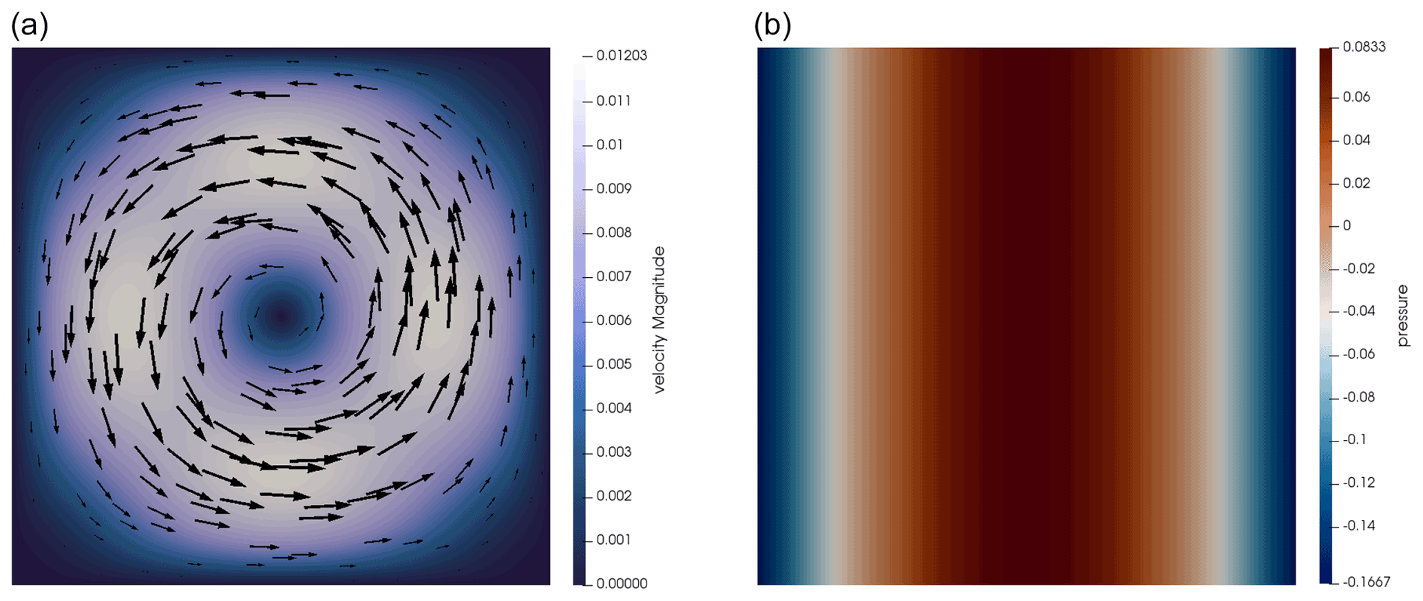
Figure 1 Donea and Huerta benchmark. Velocity (a) and pressure (b) fields obtained on a 32×32 mesh with Q₂×Q₁ elements.

We verify this in Fig. 2 for the four element choices of interest in this work: Q₁×P₀, stabilized Q₁×Q₁, Q₂×Q₁, and $Q_{\mathrm{2}}\times P_{-\mathrm{1}}$. Looking at the velocity error, we recover a cubic convergence rate (q=3) for the Q₂×Q₁ and $Q_{\mathrm{2}}\times P_{-\mathrm{1}}$ elements and a quadratic convergence rate (q=2) for those choices using the Q₁ elements for the velocity. The pressure error is of linear rate for the Q₁×P₀ element and of quadratic rate for the Q₂×Q₁ and $Q_{\mathrm{2}}\times P_{-\mathrm{1}}$ elements. All of these are as expected. For the stabilized Q₁×Q₁, we obtain the better-than-expected rate of 1.5 already mentioned in Dohrmann and Bochev (2004); see also Sect. 3.

Figure 3 shows the root mean square velocity as a function of the mesh size as obtained with the four elements in question. Again, the second-order elements are more accurate.

These results are not surprising: the solution is smooth, and consequently one would expect to obtain optimal order convergence in all cases. One can carry out similar experiments for the SolKz benchmark (Zhong, 1996), which also has a smooth solution; we have obtained identical error convergence rates.

Finally, we also investigate the cost associated with solving this problem using the various elements. Fig. 3 shows the number of outer FGMRES iterations (Kronbichler et al., 2012) iterations of the Stokes solver as a function of the mesh size.⁵ This number is nearly constant with increasing resolution for the stable or stabilized elements, while it becomes exceedingly large for the unstable Q₁×P₀ element, reflecting the fact that lack of LBB stability corresponds to the smallest eigenvalue of the system matrix tending to zero – and thereby driving the condition number to infinity. Indeed, our linear solver does not converge in the 1000 iterations we chose as a limit for the smallest mesh sizes.

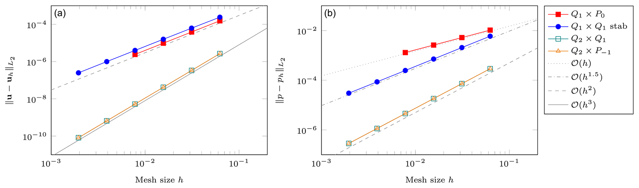
Figure 2 Donea and Huerta benchmark. Error convergence as a function of the mesh size h. (a) Velocity error $\left|\right|\mathit{u}-{\mathit{u}}_h|{|}_{L_{\mathrm{2}}}$. (b) Pressure error $\left|\right|p-p_h|{|}_{L_{\mathrm{2}}}$. The two leftmost points are missing for Q₁×P₀ since the solver failed to converge; the data points for Q₂×Q₁ and $Q_{\mathrm{2}}\times P_{-\mathrm{1}}$ are on top of each other.

Figure 3 Donea and Huerta benchmark. (a) Root mean square velocity as a function of the mesh size h. The dotted line is the analytical value. (b) Number of FGMRES solver iterations as a function of the mesh size h.

5.2 The SolCx benchmark

The SolCx benchmark is a common benchmark found in many geodynamical papers (e.g., Zhong, 1996; Duretz et al., 2011; Kronbichler et al., 2012; Thielmann et al., 2014). It uses a discontinuous viscosity profile with a large jump in the viscosity value along the middle of the domain, resulting in a discontinuous pressure field. The domain is a unit square, boundary conditions are free-slip on all edges, and the gravity vector points downwards with $\left|\mathit{g}\right|=\mathrm{1}$. The density for SolCx is given by $\mathit{\rho }(x,y)=\sin \left(\mathit{\pi }y\right)\cos \left(\mathit{\pi }x\right)$ and the viscosity field is such that

$$\mathit{\eta }(x,y)=\left\{\begin{array}{ccc}\mathrm{1},& \mathrm{if}& \mathrm{0}\le x\le \mathrm{0.5}\\ {\mathrm{10}}^{\mathrm{6}}& \mathrm{if}& \mathrm{0.5}<x\le \mathrm{1}.\end{array}\right.$$

We show the velocity and pressure fields in Fig. 4. The discontinuous jump of the viscosity field by a factor of 10⁶ results in separate convective cells on the left and right sides of the domain, though with vastly different strengths. The pressure also reflects this disjoint behavior.

As in the Donea and Huerta benchmark, we compute the velocity and pressure error convergence for all four elements. Those are shown in Fig. 5. As documented in Kronbichler et al. (2012), the second-order element with discontinuous pressure $Q_{\mathrm{2}}\times P_{-\mathrm{1}}$ performs better (pressure error convergence is 𝒪(h²)) than its continuous pressure counterpart Q₂×Q₁ (convergence is only $\mathcal{O}\left(h^{\mathrm{1}/\mathrm{2}}\right)$, but the better convergence order with the discontinuous pressure can only be obtained if the discontinuity in the viscosity is aligned with cell boundaries – which is the case here. Also of interest here is the fact that the Q₁×P₀ outperforms the Q₁×Q₁ element for both velocity and pressure. All of these observations are readily explained by the fact that a discontinuous pressure can only be approximated well when using discontinuous pressure elements with cell interfaces aligned with the discontinuity in the viscosity.

Figure 6 shows the number of outer FGMRES iterations of the Stokes solver as a function of the mesh size. We find this time that this number is nearly constant with increasing resolution for all four elements. Unsurprisingly the Q₁×P₀ element requires more iterations than all the others but by less than a factor of 2. The quadratic elements require the same number of iterations, while the stabilized Q₁×Q₁ requires only half their number: this is surprising, but the conclusions from the previous paragraph remain about it being the least accurate of all four elements here.

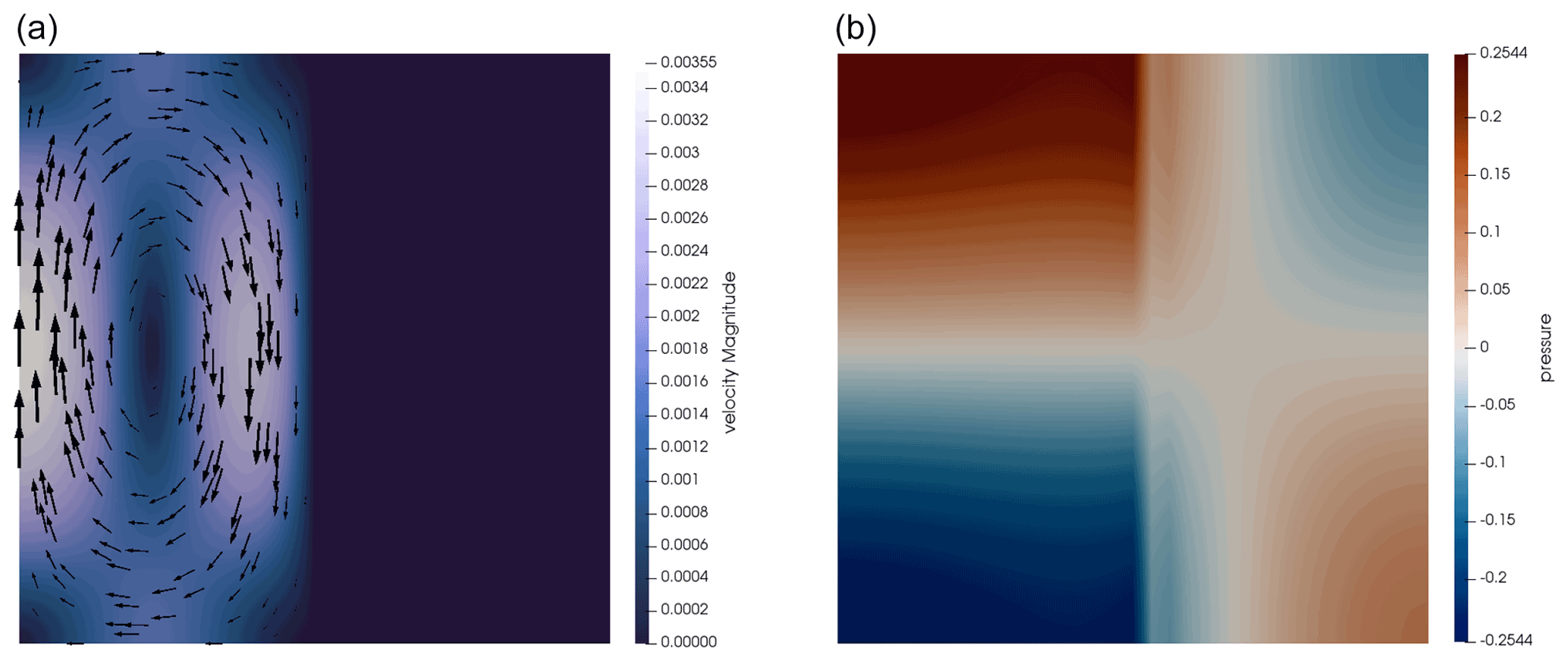
Figure 4 SolCx benchmark. Velocity (a) and pressure (b) fields obtained on a mesh with a resolution of 32×32 grid with the Q₂×Q₁ element.

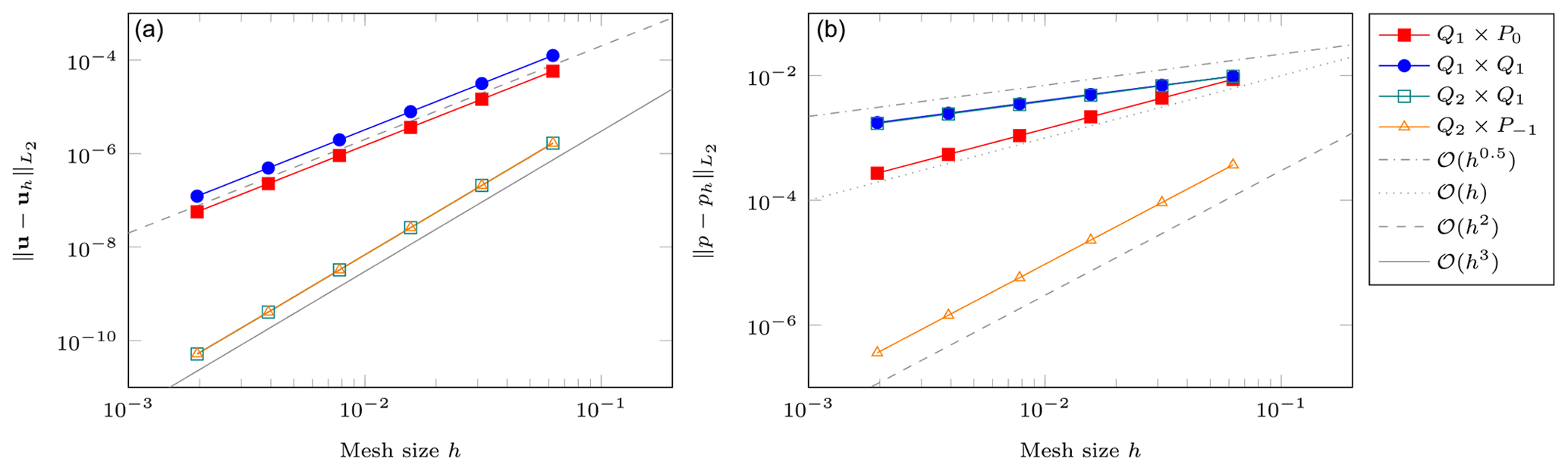
Figure 5 SolCx benchmark. Error convergence as a function of the mesh size h. (a) Velocity error; (b) pressure error.

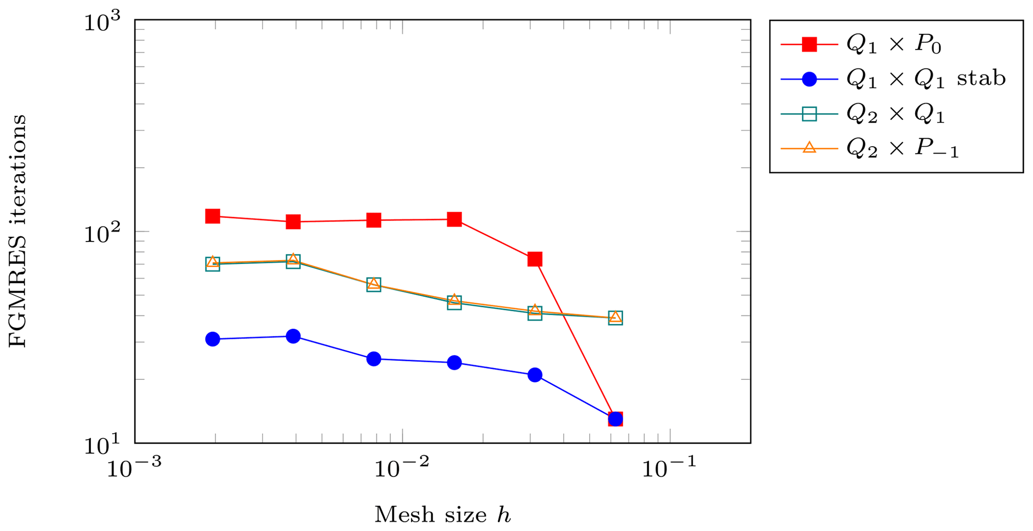
Figure 6 SolCx benchmark. Number of FGMRES solver iterations as a function of the mesh size h.

5.3 The SolVi (circular inclusion) benchmark

The SolCx benchmark in the previous section allows for aligning mesh interfaces with the discontinuity in the viscosity. This is an artificial situation that will, in general, not happen in actual large-scale geodynamics applications for which the interfaces between materials may be at arbitrary locations and orientations in the domain and may also move with time. An example is the simulation of a cold subducting slab (with correspondingly large viscosity) surrounded by hot low-viscosity mantle material. Consequently, it is worth considering a situation in which it is impractical to align mesh and viscosity interfaces. This is done by the SolVi inclusion benchmark, which solves a problem with a viscosity that is discontinuous along a circle. This in turns leads to a discontinuous pressure along the interface, which is difficult to represent accurately. Using the regular meshes used by a majority of codes, the discontinuity in the viscosity and pressure then never aligns with cell boundaries. Even though Aspect can use arbitrary unstructured meshes (and can also use curved cell edges), we will honor the setup of this benchmark by only considering regular meshes.

Schmid and Podlachikov (2003) derived a simple analytical solution for the pressure and velocity fields for such a circular inclusion under pure shear, and this benchmark is showcased in many publications (Deubelbeiss and Kaus, 2008; Suckale et al., 2010; Duretz et al., 2011; Kronbichler et al., 2012; Gerya et al., 2013; Thielmann et al., 2014). The velocity and pressure fields are shown in Fig. 7.

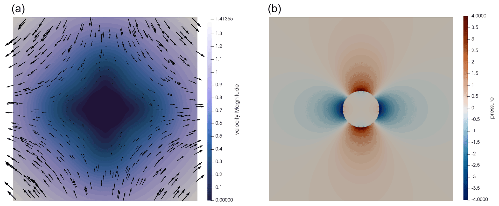
Figure 7 SolVi benchmark with inclusion of radius 0.2. Velocity (a) and pressure (b) fields obtained on a 256×256 mesh using Q₂×Q₁ elements.

A characteristic of the analytic solution is that the pressure is zero inside the inclusion, while outside it follows the relation

$$\begin{array}{}\text{(14)}& p=\mathrm{4}\dot{\mathit{ϵ}}{\displaystyle \frac{{\mathit{\eta }}_{\mathrm{m}}({\mathit{\eta }}_{\mathrm{i}}-{\mathit{\eta }}_{\mathrm{m}})}{{\mathit{\eta }}_{\mathrm{i}}+{\mathit{\eta }}_{\mathrm{m}}}}{\displaystyle \frac{r_{\mathrm{i}}^{\mathrm{2}}}{r^{\mathrm{2}}}}\cos \left(\mathrm{2}\mathit{\theta }\right),\end{array}$$

where η_i=10³ is the viscosity of the inclusion, η_m=1 is the viscosity of the background medium, $r=\sqrt{x^{\mathrm{2}}+y^{\mathrm{2}}}$, $\mathit{\theta }=\arctan (y/x)$, and $\dot{\mathit{ϵ}}=\mathrm{1}$ is the applied strain rate if one were to extend the domain to infinity. The formula above makes it clear that the pressure is discontinuous along the perimeter of the disk, with the jump largest at $\mathit{\theta }=\mathrm{0},\pm \frac{\mathit{\pi }}{\mathrm{2}},\mathit{\pi }$.

Deubelbeiss and Kaus (2008) thoroughly investigated this problem with various numerical methods (FEM, FDM), with and without tracers, and conclusively showed how various schemes of averaging the density and viscosity lead to different results. Heister et al. (2017) also come to this conclusion and also considered how averaging the coefficient on each cell affects the number of iterations necessary to solve the linear systems. We repeat these experiments here but with our larger set of different elements. Specifically, results obtained with no averaging inside the element (“No”), arithmetic averaging (“Arith”), geometric averaging (“Geom”), and harmonic averaging (“Harm”) are shown in Fig. 8. We see that (i) all four elements show the same rate of convergence: 𝒪(h) for velocity errors and 𝒪(h^0.5) for pressure errors; (ii) harmonic averaging always yields lower errors, validating the findings of Heister et al. (2017); (iii) the number of iterations in the Stokes solver is the lowest for the stabilized Q₁×Q₁ element; and (iv) this number is not strongly affected by the method of averaging (with the exception of the $Q_{\mathrm{2}}\times P_{-\mathrm{1}}$ element). The observation that none of the elements reach their optimal convergence rate also supports our decision, briefly mentioned in the “Goals of this paper” part of the Introduction, to not further investigate higher-order Taylor–Hood elements $Q_k\times Q_{k-\mathrm{1}}$ or $Q_k\times P_{-(k-\mathrm{1})}$ with k>2: we know from experiments such as the current one that these elements will not yield better convergence orders despite their additional cost.

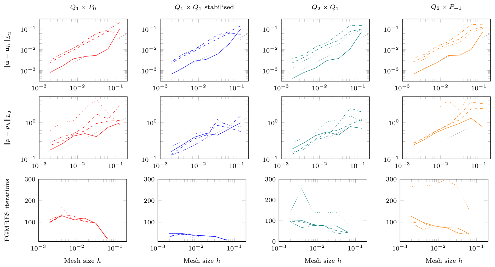
Figure 8 SolVi benchmark. Left to right: Q₁×P₀, stabilized Q₁×Q₁, Q₂×Q₁, and $Q_{\mathrm{2}}\times P_{-\mathrm{1}}$. Top to bottom: velocity error, pressure error, and number of FGMRES iterations for the Stokes solve. The individual lines in each graph correspond to different ways of averaging coefficients on each cell: dotted lines use the correct unaveraged values of coefficients at each quadrature point; dash-dotted lines compute the arithmetic average of the values at the quadrature points on a cell and use the average for all quadrature points; dashed lines use the geometric average; solid lines use the harmonic average. The gray dotted line in the first two rows indicates 𝒪(h) convergence for velocity and 𝒪(h^0.5) for pressure.

Since harmonic averaging yields the lowest errors we select this averaging and now turn to the pressure field for all elements as shown in Fig. 9. We find that the recovered pressures on the line y=1 follow the analytical solution outside the inclusion but are less accurate inside the inclusion where it should be identically zero (Fig. 10).

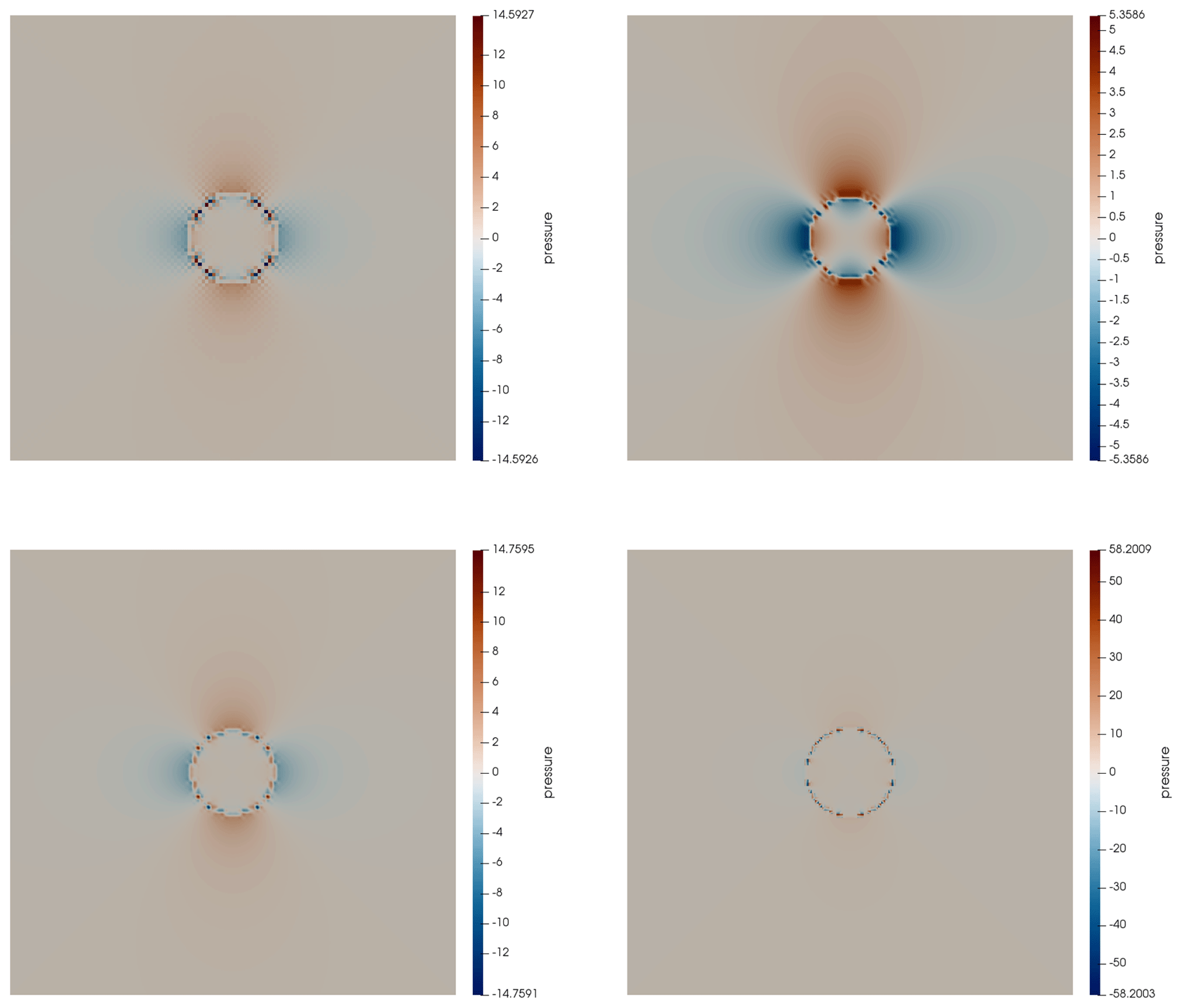
Figure 9 SolVi benchmark. Pressure field for the Q₁×P₀, stabilized Q₁×Q₁, Q₂×Q₁, and $Q_{\mathrm{2}}\times P_{-\mathrm{1}}$ elements from left to right and top to bottom at resolution 128×128 with no averaging. Note the different color scales, illustrating the differing size of overshoots and undershoots for the different discretizations.

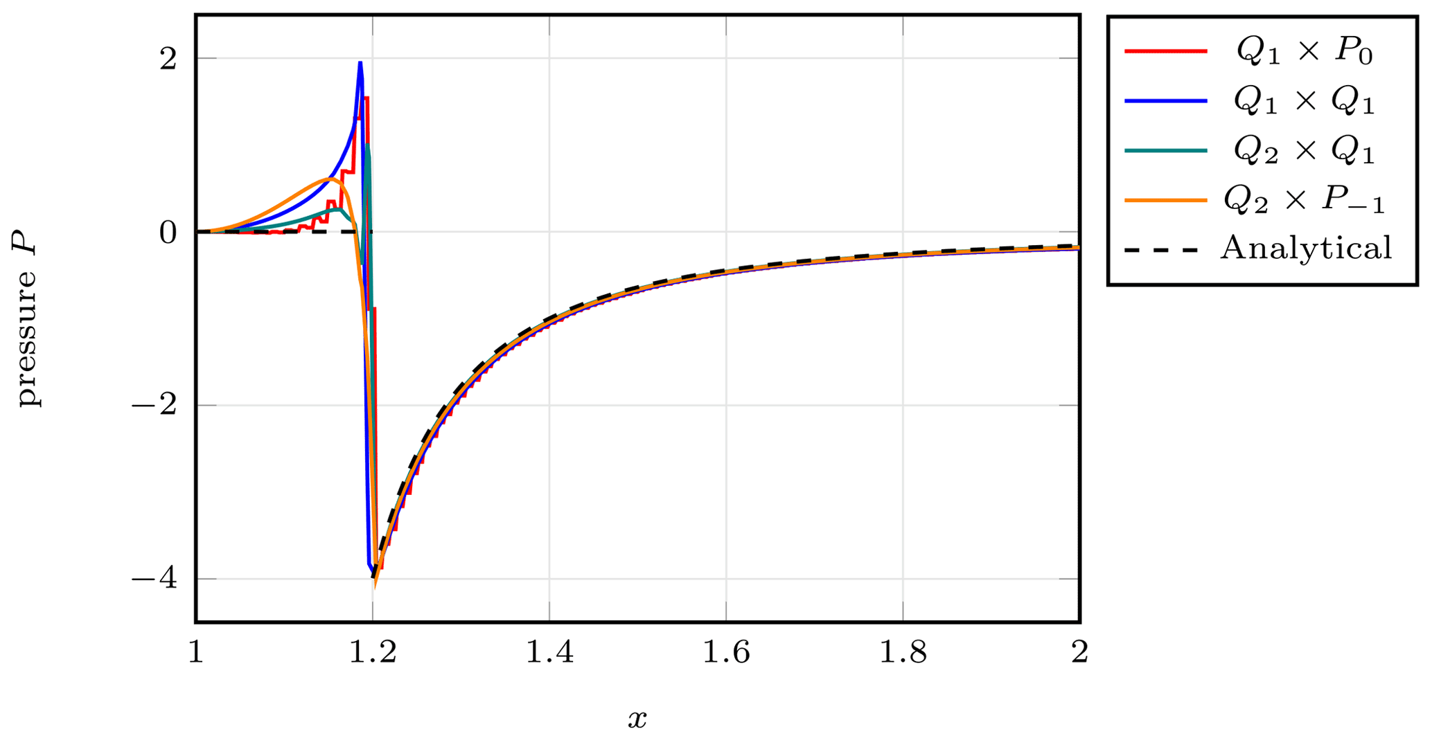
Figure 10 SolVi benchmark. Pressure on the horizontal ray starting from the center of the inclusion at x=1.

5.4 The sinking block

As discussed in Sect. 4, the stabilized Q₁×Q₁ element is sensitive to the choice of a reference density profile as not only the computed pressure, but also the computed velocity field, depends on this choice. This is only relevant for buoyancy-driven flows, but because none of the benchmarks shown previously are driven by buoyancy effects in the presence of a background lithostatic pressure to any significant degree, let us next consider a setup in which this is the dominant effect. To this end, we perform an experiment based on a benchmark similar or identical to the ones presented in May and Moresi (2008), Gerya (2019), Thieulot (2011), and Schuh-Senlis et al. (2020).

It consists of a two-dimensional 512×512 km domain filled with a fluid (the “mantle”) of density ρ₁=3200 kg m⁻³ and viscosity η₁=10²¹ Pa s. A square block of size 128×128 km is placed in the domain and is centered at location (x_c, y_c) = (256, 384 km) so as to ensure that its sides align with cell boundaries at all resolutions, avoiding cases in which the quadrature within one element corresponds to different density or viscosity values. It is filled with a fluid of density ${\mathit{\rho }}_{\mathrm{2}}={\mathit{\rho }}_{\mathrm{1}}+\mathit{\delta }\mathit{\rho }$ and viscosity η₂. The gravity vector points downwards with $\left|\mathit{g}\right|=\mathrm{10}$ m s⁻². Boundary conditions are free-slip on all sides. The pressure null space is removed by enforcing ${\int }_{\mathrm{\Omega }}p\mathrm{d}V=\mathrm{0}$, and only one time step is carried out. The benchmark then solves for the instantaneous pressure and velocity field for this setup.

In a geodynamical context, the block could be interpreted as a detached slab (δρ>0) or a plume head (δρ<0). As such its viscosity and density can vary (a cold slab has a higher effective viscosity than the surrounding mantle, while it is the other way around for a plume head). The block density difference δρ can then vary from a few to several hundred kilograms per cubic meter (kg m⁻³) to represent a wide array of scenarios. As shown in Appendix A.2 of Thieulot (2011), one can independently vary η₁, ρ₂, and η₂ and measure $\left|v_z\right|$ for each combination: the quantity $\mathit{\nu }=\left|v_z\right|{\mathit{\eta }}_{\mathrm{1}}/\mathit{\delta }\mathit{\rho }$ is then found to be a simple function of the ratio ${\mathit{\eta }}^{\star }={\mathit{\eta }}_{\mathrm{2}}/{\mathit{\eta }}_{\mathrm{1}}$. At high enough mesh resolution all data points collapse onto a single line.

In the following, we will denote as Method 1 the approach whereby we do calculations with the density field as specified above. Method 2 consists of a “reduced” density field from which the quantity ρ₁ has been uniformly removed so that the block has a density δρ, while the surrounding fluid has zero density. As discussed above, the two choices will result in different pressure but the same velocity fields.

We have carried out measurements for all four elements with ${\mathit{\eta }}^{\star }\in [{\mathrm{10}}^{-\mathrm{4}}:{\mathrm{10}}^{\mathrm{6}}]$ and $\mathit{\delta }\mathit{\rho }/{\mathit{\rho }}_{\mathrm{1}}\in \mathit{\{}\mathrm{0.25}\mathit{\%},\mathrm{1}\mathit{\%},\mathrm{4}\mathit{\%}\mathit{\}}$ corresponding to $\mathit{\delta }\mathit{\rho }\in \mathit{\{}\mathrm{8},\mathrm{32},\mathrm{128}\mathit{\}}$ kg m⁻³. Results for $\mathit{\nu }=f\left({\mathit{\eta }}^{\star }\right)$ for all elements, the three block density values, and five different mesh resolutions are shown in Fig. 11 for the two methods.

When using the full density, we see that all elements, with the exception of the stabilized Q₁×Q₁ element, yield results which align on a single curve on the plots once sufficient resolution is reached. We find that measurements pertaining to a given resolution but different δρ are always collapsed onto a single line. It is worth noticing that the $Q_{\mathrm{2}}\times P_{-\mathrm{1}}$ element results seem to be the least resolution-dependent. On the other hand, the stabilized Q₁×Q₁ element yields very anomalous results which are orders of magnitude off at all resolutions, especially for ${\mathit{\eta }}_{\mathrm{1}}/{\mathit{\eta }}_{\mathrm{2}}\gg \mathrm{1}$. In addition, we find that for this element, the value of δρ strongly affects the measurements, as expected based on the discussions in Sect. 4; as a result, the curves for the same mesh resolution but different δρ₂ no longer coincide (see Fig. 11b).

When reduced densities are used results are unchanged for the stable elements (only Q₂×Q₁ results are shown in Fig. 11e), and the results for the stabilized Q₁×Q₁ results are substantially improved. For values ${\mathit{\eta }}_{\mathrm{1}}/{\mathit{\eta }}_{\mathrm{2}}<\mathrm{1}$ we see that all results align on the expected curve, but this is far from true for ${\mathit{\eta }}_{\mathrm{1}}/{\mathit{\eta }}_{\mathrm{2}}\gg \mathrm{1}$ even at high resolution.

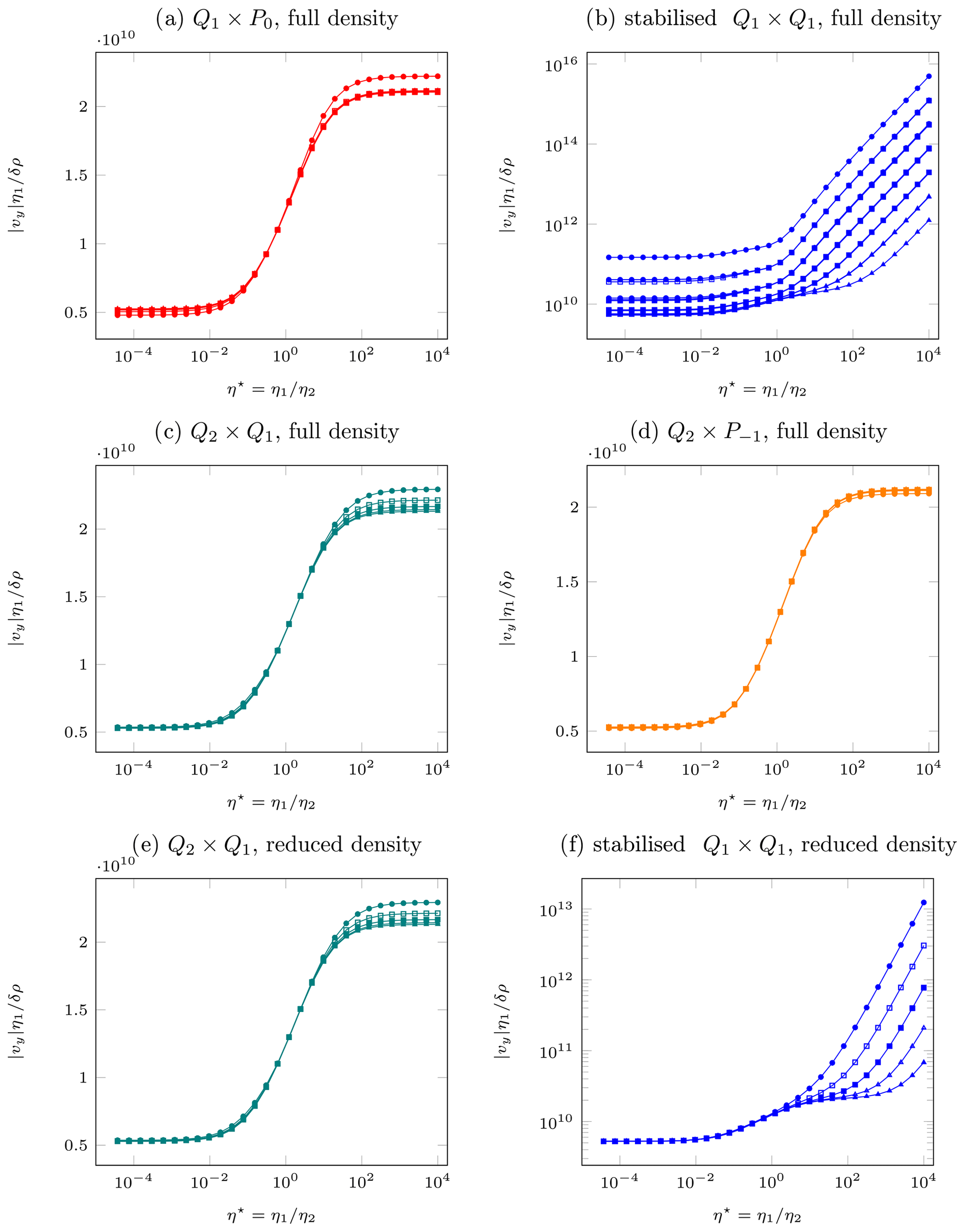
Figure 11 Sinking block benchmark. (a–d) $\mathit{\nu }=\left|v_z\right|{\mathit{\eta }}_{\mathrm{1}}/\mathit{\delta }\mathit{\rho }$ as a function of ${\mathit{\eta }}^{\star }={\mathit{\eta }}_{\mathrm{2}}/{\mathit{\eta }}_{\mathrm{1}}$ as obtained with the four elements with full density; (e, f) same with reduced density for only two element types. Legend: • 16×16 resolution, □ 32×32 resolution, ▪ 64×64 resolution, △ 128×128 resolution, ▴ 256×256 resolution. Colors represent the element used. For each mesh resolution, we show separate curves for $\mathit{\delta }\mathit{\rho }/{\mathit{\rho }}_{\mathrm{1}}\in \mathit{\{}\mathrm{0.25}\mathit{\%},\mathrm{1}\mathit{\%},\mathrm{4}\mathit{\%}\mathit{\}}$; for all but the stabilized Q₁×Q_q element, these curves coincide. Note the different y axis used for the stabilized Q₁×Q₁ element in (b) and (f).

In Fig. 12 we show the velocity field in the case ${\mathit{\eta }}^{\star }={\mathrm{10}}^{-\mathrm{4}}$ (i.e., the viscosity of the block is 10 000 times smaller than the surrounding mantle) and δρ=8 kg m⁻³. When the Q₂×Q₁ element is employed in conjunction with Method 1 we see in Fig. 12a that the velocity field is strongest inside the block with a maximum value of about 5 mm yr⁻¹ in its center. We see that the Q₂×Q₁ and $Q_{\mathrm{2}}\times P_{-\mathrm{1}}$ elements yield nearly identical results (Fig. 12b), so we consider this to be the correct solution of the physical experiment. The same setup with the stabilized Q₁×Q₁ (left half of Fig. 12c) yields a velocity field that is also maximal in the middle of the block but nearly 1000 times larger in amplitude. If we now switch to Method 2 (right half of Fig. 12c) the amplitude of the velocity is reduced by 2 orders of magnitude, but it is still much too large compared to the true solution.

These observations illustrate the unreliable nature of the results obtained with stabilized Q₁×Q₁ elements in the context of buoyancy-driven flows. Looking at Fig. 11f we see that increasing the resolution to 512×512 or 1024×1024 would probably yield the expected curve, but such resolutions are intractable in three dimensions and better results can be obtained at much lower resolutions with other elements.

Figure 12 Sinking block benchmark with $\mathit{\delta }\mathit{\rho }/\mathit{\rho }=\mathrm{0.25}$ % and ${\mathit{\eta }}^{\star }={\mathrm{10}}^{\mathrm{4}}$ on a 256 × 256 element mesh. (a) Viscosity and velocity field. (b) Velocity field obtained with the Q₂×Q₁ element (left of vertical white line) and $Q_{\mathrm{2}}\times P_{-\mathrm{1}}$ element (right of vertical line), both using full density; (c) velocity field obtained with stabilized Q₁×Q₁ with full density (left) and stabilized Q₁×Q₁ with reduced density (right).

Finally, in Fig. 13 we plot the normalized pressure $p^{\star }=p/\left(\mathit{\delta }\mathit{\rho }g{L}_{\mathrm{b}}\right)$ at the center of the block (where L_b is the size of the block) as a function of the viscosity ratio η^⋆ in the case in which a reduced density field is used. For the Q₂×Q₁ and the stabilized Q₁×Q₁ elements, the pressure at this point is uniquely defined since the elements have continuous pressures. For the other two elements the pressure is discontinuous across element edges, and it is therefore not uniquely defined at our measurement point. We have then chosen to measure it at four locations corresponding to $(x_{\mathrm{c}}\pm \mathit{\delta }x,y_{\mathrm{c}}\pm \mathit{\delta }y)$, where $\mathit{\delta }x=\mathit{\delta }y=\mathrm{0.1}$ m, and show the normalized pressures at all four of these locations in the figure. For the $Q_{\mathrm{2}}\times P_{-\mathrm{1}}$ element, the difference between these values is negligible but not so for the Q₁×P₀ for which the pressure is a stairstep function with very different values depending on which step an evaluation point is on. The distance between the two lines for the Q₁×P₀ element decreases with mesh refinement (indicating convergence of the pressure to the true value), but only slowly and, matching the observation in Sect. 5.1, at the cost of not only a fine mesh but also very large numbers of linear solver iterations.

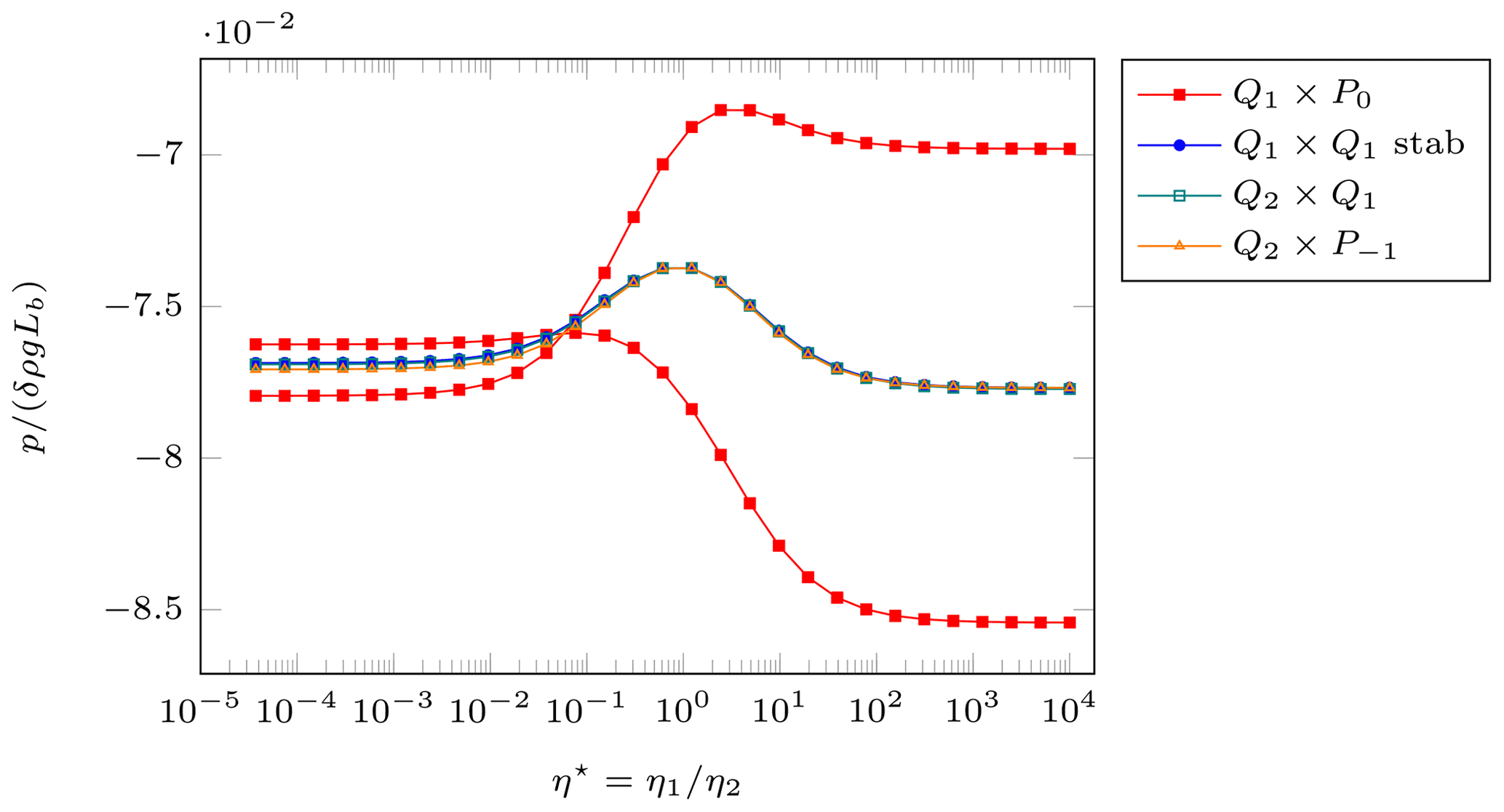
Figure 13 Sinking block benchmark. Normalized pressure $p/\left(\mathit{\delta }\mathit{\rho }g{L}_{\mathrm{b}}\right)$ in the center of the block as a function of the viscosity ratio η^⋆. These computations use a 256 × 256 mesh and the reduced density. For the Q₁×P₀ and $Q_{\mathrm{2}}\times P_{-\mathrm{1}}$ elements with their discontinuous pressure spaces, we show the normalized pressures at several slightly displaced points $(x_{\mathrm{c}}\pm \mathit{\delta }x,y_{\mathrm{c}}\pm \mathit{\delta }y)$. For the $Q_{\mathrm{2}}\times P_{-\mathrm{1}}$ element, the difference is not visible, but for the Q₁×P₀ this yields the two very different red curves; this is due to the fact that the pressure for this element forms a stairstep function for which two of the evaluation points are on a lower and two on a higher step.

In addition to the slow convergence of the Q₁×P₀ element, the most striking conclusion of this benchmark is that for buoyancy-driven flows, the solution obtained using the stabilized Q₁×Q₁ element on typical meshes not only strongly depends on the choice of the otherwise arbitrary reference density, but is also almost entirely unreliable even on meshes that are already quite fine.

6 Numerical results for a model application

While the previous sections have built our intuition for which element may actually work in the context of geodynamics applications, they have only done so through abstract and idealized benchmarks. It is therefore interesting to investigate what one would find in more realistic setups, and consequently we have also investigated convergence for a situation still sufficiently simple that numerical simulations can reach reasonably high accuracy but that has more of the complexity one would generally find in “real” simulations. Given that the previous examples have highlighted the fact that the stabilized Q₁×Q₁ element has difficulties with the pressure approximation, we are specifically interested in a situation in which the material behavior is pressure-dependent.

To this end, we consider an example of continental extension here. The setup is similar to ones that can be found in Huismans and Beaumont (2002), Jammes and Huismans (2012), Naliboff and Buiter (2015), and Brune et al. (2017), and we specifically use the one that can be found in the “continental extension” cookbook of the manual of the Aspect code (Bangerth et al., 2022). The situation we model here is characterized by the following building blocks: on a domain of size 400 km × 100 km, we impose an extensional horizontal velocity component of ±0.25 cm yr⁻¹ on the sides and a vertical upward velocity of 0.125 cm yr⁻¹ at the bottom. The tangential components are left free. At the top, we allow for a free boundary. More interestingly, we use a pressure- and temperature-dependent viscoplastic rheology of Drucker–Prager type with parameters for viscous deformation based on dislocation creep flow laws:

$$\begin{array}{}\text{(15)}& {\mathit{\eta }}_{\mathrm{disl}}=A^{-\mathrm{1}/n}{\dot{\mathit{\epsilon }}}^{-\mathrm{1}+\mathrm{1}/n}\exp \left({\displaystyle \frac{Q+pV}{nRT}}\right),\end{array}$$

where A is a material constant, n is an index typically between 3 and 4, Q is the activation energy, V is the activation volume, R the gas constant, T the temperature, and $\dot{\mathit{\epsilon }}$ is the effective strain rate (the square root of the second invariant of the corresponding tensor). Stresses are limited plastically at a yield stress ${\mathit{\sigma }}_y=C\cos \left(\mathit{\varphi }\right)+P\sin \left(\mathit{\varphi }\right)$ via a Drucker–Prager criterion where C is the cohesion and ϕ the angle of friction. We use distinct values for some of these parameters in the initially 20 km thick upper crust (wet quartzite), an initially 10 km thick lower crust (wet anorthite), and the mantle (dry olivine), which initially occupies the remaining 70 km in depth. Deformation is seeded by a weak area within the mantle lithosphere. We only carry out a single time step as obtained with a CFL number of 0.5.

A complete and concise description of this setup has more parameters than are worth spelling out in detail here. For a detailed description, see Naliboff and Buiter (2015) and the section of the Aspect manual along with the corresponding input files. For the purposes of this paper, the important part is that both the yield stress and the dislocation creep rheology depend on the pressure; as a consequence, we can anticipate that elements that result in poor pressure accuracy may not yield accurate simulations in general.

This setup produces localized shear zones that accommodate the majority of the deformation. Figure 14 illustrates the structure of the resulting solution. Each panel of the figure shows in its left half the solution produced by the stabilized Q₁×Q₁ element and its right half that produced by the Taylor–Hood Q₂×Q₁ element. Because the solution is symmetric, the two halves should be mirror images. It is, however, clear from several of the panels that this is not the case: the Q₁×Q₁ element produces large artifacts at depth where the pressure is large and the pressure dependence of the material strong.

Figure 14 Application example. (a) Vertical component of the velocity field; (b) pressure field; (c) effective viscosity field; (d) effective strain rate field. In all panels, the left half (left of the vertical line) shows data obtained with the stabilized Q₁×Q₁ element, whereas the right half shows results obtained with the Q₂×Q₁ element. Note the large deviations between the two towards the bottom of the domain. All results were obtained on an 800×200 mesh with a cell size of 0.5 km.

This effect is also demonstrated in a different way in Fig. 15 where we show laterally averaged quantities for the different elements and different mesh resolutions. Even though it is clear from Fig. 14 that lateral averaging should result in a better approximation (than pointwise evaluations) of the correct quantities for a given depth, Fig. 15 shows that even the average is far from correct. On the other hand, the figure shows that with increasing mesh resolution, the solutions produced by the Q₁×Q₁ seem to converge to the solutions generated by the other elements – albeit very slowly and at what one might consider an unacceptable cost.

Figure 15 Application example. (a) Laterally averaged effective viscosity; (b) laterally averaged velocity magnitude. The line styles chosen become increasingly assertive (dotted to solid lines) as mesh resolution is increased.

To investigate the origin of these convergence problems of the Q₁×Q1 element, one should recall that the model is nonlinear. As a consequence, the artifacts may be related to the discretization or to a failure of the nonlinear iteration – and the two may be connected. All of the solutions we show were taken after 100 Picard iterations to resolve the nonlinearity of the model, with nonlinear convergence shown in Fig. 16. (One could accelerate convergence by using a Newton solver – Fraters et al., 2019 – but this is not relevant for the work herein.) Looking at the evolution of the nonlinear residual during these iterations, we see that it decreases quickly and for most element choices then plateaus at about 10⁻⁵ relative to the starting residual. In contrast, for the stabilized Q₁×Q₁ element, increasing the mesh resolution yields lower nonlinear residuals – but even on the finest mesh, the nonlinear residuals are still substantially worse than for any of the other elements, with no apparent progress after about 20 iterations. Of course, we are not the first to observe that convergence is hard to come by for these sorts of problems (see, for example, Spiegelman et al., 2016), and recent approaches to regularize visco(–elasto)–plastic deformation by Duretz et al. (2020) and Jacquey et al. (2021) have been found to improve the convergence behavior of the nonlinear solvers.

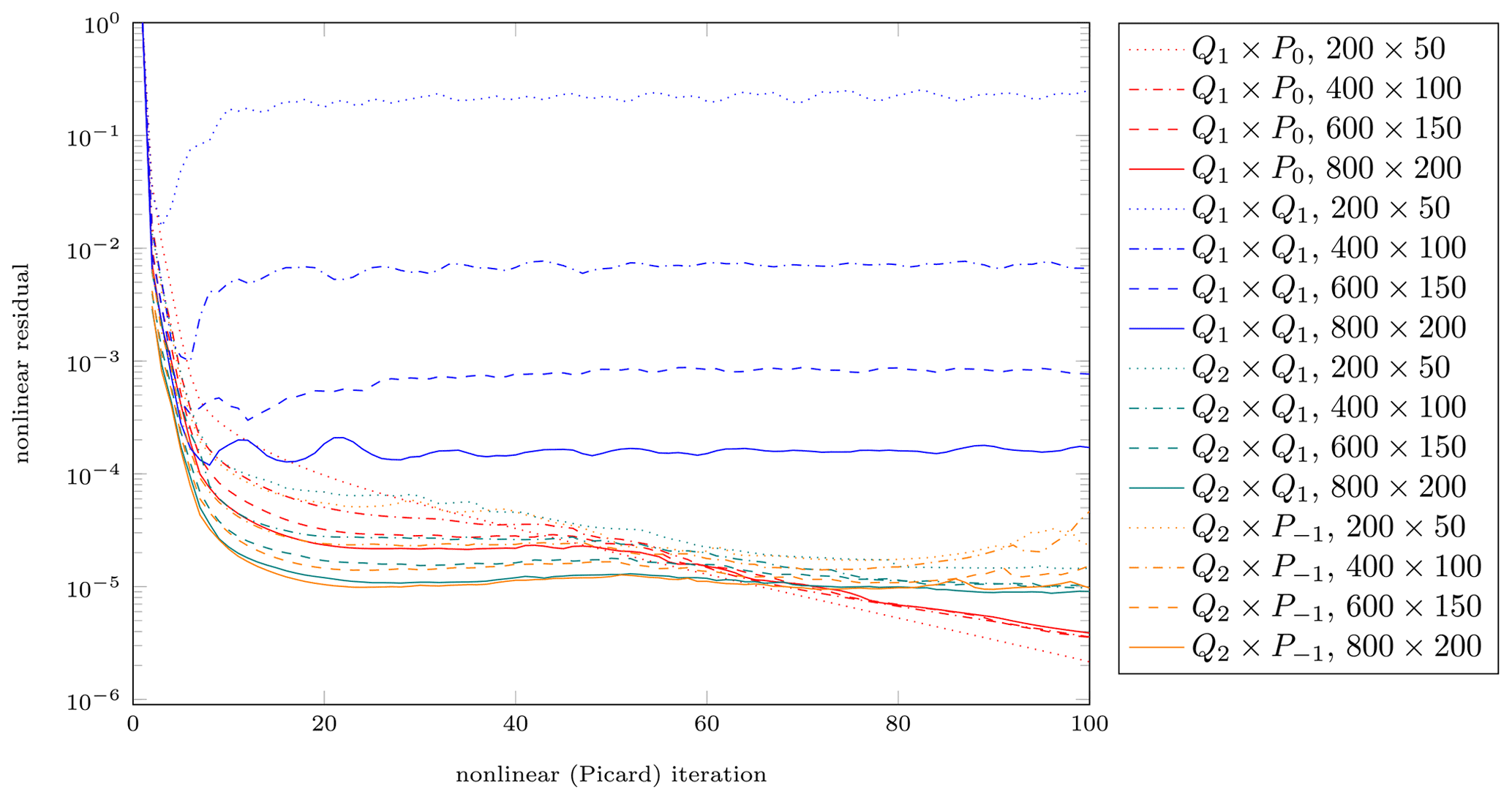
Figure 16 Application example. Nonlinear residual as a function of nonlinear iteration step for all four elements and for different mesh resolutions.

Our interpretation of this experiment is that the inability of the Q₁×Q₁ element to generate accurate pressure fields leads to values for the pressure-dependent rheology that are so far away from their correct values – and, indeed, from the values on nearby cells – that they greatly increase the condition number of the linear systems that have to be solved in each nonlinear iteration. The resulting difficulty of solving these Picard steps accurately then affects the speed with which the nonlinear residual is reduced by the Picard iteration to the point at which the condition number is so large that convergence can no longer be achieved. Only mesh refinement, with the attendant increased accuracy of the pressure solution (and, consequently, a more accurate viscosity), helps to restore the ability to actually solve this problem to small nonlinear residuals.

7 Conclusions

In this contribution, we have provided a side-by-side comparison of the most widely used quadrilateral finite elements. As outlined in the Introduction, most finite-element solvers used in the geodynamics community rely on one or the other of these. At the same time, we are not aware of a comprehensive comparison of their relative strengths – or their weaknesses, as they may be.

Using the artificial linear benchmarks discussed in Sect. 5, we can infer that when the solution is smooth, the Taylor–Hood variations Q₂×Q₁ and $Q_{\mathrm{2}}\times P_{-\mathrm{1}}$ provide far better accuracy than the lower-order elements Q₁×P₀ and the stabilized Q₁×Q₁. This advantage is largely lost when one considers problems in which the viscosity is discontinuous. Since we believe that the real Earth has relatively narrow phase transition zones where the viscosity may jump by large factors, benchmarks like the SolVi one in Sect. 5.3 are relevant and illuminate important aspects.

From these considerations, one may conclude that the Taylor–Hood variations are too expensive – in terms of their number of degrees of freedom and the attendant memory and CPU time cost. However, we believe that this is not so.

• For buoyancy-driven flows such as the sinking block benchmark in Sect. 5.4, the stabilized Q₁×Q₁ element is largely unable to reproduce the correct solution and, furthermore, depends on using a formulation in which one subtracts a reference density from the actual density; this is equivalent to defining a hydrostatic pressure profile and only attempting to solve for the “dynamic” component of the pressure. Crucially, however, there are many ways of defining such a reference density, neither of which is canonical and “obviously right” in complex mantle convection simulations. Since the solution obtained with the stabilized Q₁×Q₁ element strongly depends on the specific choice of reference density, we conclude that the element cannot be made robust for the kinds of flows we encounter in real mantle convection situations. We have also verified this assertion using an application in which we consider continental extension (Sect. 6) and in which the inability to produce accurate pressure solutions also greatly affects the convergence of the nonlinear solver to the point at which the computed solution must be considered unusable. We have shown that these errors can be reduced when choosing very fine meshes, but the attendant cost is unacceptable when compared with that of using other elements on far coarser meshes.

  There are other considerations to believing that the procedure of trying to subtract a reference density (or a hydrostatic pressure) cannot be a successful strategy. For example, simulations of free or deformable surfaces (at the Earth's surface as well as at the core–mantle boundary) require accurate knowledge of the total pressure. This is true for coupled formulations of flow and surface deformation (Rose et al., 2017) as well as approaches such as the “sticky air” method (Crameri et al., 2012). But similar considerations also apply to nonlinear material laws in which the pressure enters the viscosity or, more commonly, phase computations that determine the density and other thermodynamic material properties from the pressure and the temperature. Indeed, one could conjecture that the stabilized Q₁×Q₁ element would also fail for compressible Stokes simulations, though we have not verified this here.

  We conclude from these thoughts that the stabilized Q₁×Q₁ element is not a viable choice for mantle convection simulations. It is important to point out that the cases we consider to be crucial here – buoyancy-driven flows, large hydrostatic pressures, and pressure-dependent rheologies – are uncommon in most of the engineering applications for which the Q₁×Q₁ was originally developed; as a consequence, it is not surprising that what we find here contradicts substantial parts of the engineering literature wherein the element remains widely used.

• We believe that the Q₁×P₀ element is also not a viable choice. As shown by several of the analytical benchmarks, the errors that result from using this element can be orders of magnitude larger than the corresponding errors that result from the Taylor–Hood-type elements. This is no longer the case once we consider discontinuous viscosity profiles (see Sect. 5.3), but this element is also unable to accurately solve the buoyancy-driven case discussed in Sect. 5.4. Furthermore, as pointed out before, this element is not LBB-stable, which, despite considerable efforts in the past decades, has limited its use in combination with iterative methods: because of the corresponding condition number increase, the number of iterations is found to grow in a somewhat unpredictable manner with an increase in resolution. This may explain why, despite the Citcom codes' success over 2 decades with studies based on models counting up to ∼ 100 million elements on several hundred processors (e.g., Jadamec and Billen, 2012), the current generation of massively parallel codes relies on either stable (Kronbichler et al., 2012; May et al., 2015) or stabilized elements (Burstedde et al., 2013), or they use the finite-difference method (Kaus et al., 2016).

In summary, we think that the Taylor–Hood variations Q₂×Q₁ and $Q_{\mathrm{2}}\times P_{-\mathrm{1}}$ present the best compromise for robust mantle convection and crustal dynamics simulations based on the finite-element method. This is not because these elements are “obviously better” than the others but due more to a “last man standing” argument: the other choices simply disqualified themselves by failing to provide adequate accuracy in one situation or another. At the same time, the lack of regularity one expects of typical scenarios also implies that we should not expect higher-order Taylor–Hood elements $Q_{k+\mathrm{1}}\times Q_k$ or $Q_{k+\mathrm{1}}\times P_{-k}$ with k>2 to provide substantially better accuracy compared to their much higher computational cost. Although we have only shown results for two-dimensional simulations, experience – including the experience with the Aspect code used here that solves two- and three-dimensional problems within the same framework – suggests that all of these considerations would also apply to the three-dimensional (hexahedral) analogs of the ones we have used.

The experiments we have shown do not provide clear guidance on whether one should use the Q₂×Q₁ or $Q_{\mathrm{2}}\times P_{-\mathrm{1}}$ element. But other considerations can provide such guidance. Most notably, the elements with discontinuous pressure elements (namely, the $Q_{\mathrm{2}}\times P_{-\mathrm{1}}$ but also the Q₁×P₀ elements) have the “local conservation” property for which the velocity satisfies

$${\displaystyle }\underset{K}{\int }\mathrm{\nabla }\cdot {\mathit{u}}_h=\underset{\partial K}{\int }\mathit{n}\cdot {\mathit{u}}_h=\mathrm{0}$$

on every cell K of the mesh, a property also satisfied by the exact solution. Local conservation is useful when considering that the velocity computed in geodynamics models is often used in a second step to advect both the temperature field and chemical compositions (see, for example, Schubert et al., 2001). A comprehensive investigation of the interplay of local conservation and transport can be found in Dawson et al. (2004).

Of course, the choices we have considered here are not the only ones. One could, for example, consider “simplicial” (triangular and tetrahedral) elements instead of the quadrilateral and hexahedral ones we have used here. Indeed, some existing mantle convection codes use this strategy. One successful example is the TERRA-NEO code that uses equal-order linear tetrahedra (Gmeiner et al., 2015; Weismüller et al., 2015) stabilized by means of a pressure-stabilization approach based on the addition of linear least-squares terms (the “PSPG” approach, see Brezzi and Douglas, 1988; Elman et al., 2014); other examples include Fluidity (Davies et al., 2011), MILAMIN (Dabrowski et al., 2008), and LaCoDe (de Montserrat et al., 2019). While we have not evaluated simplicial elements, one might conjecture that many of the same conclusions would also hold: the unstable P₁×P₀ provides low accuracy and is unstable, the stabilized P₁×P₁ has difficulties with buoyancy-driven flows and large hydrostatic pressures, and the Taylor–Hood element P₂×P₁ is expensive but robust.

Finally, there are other more exotic elements one could work with. Examples include the Rannacher–Turek element (Rannacher and Turek, 1992), the Crouzeix–Raviart element (Crouzeix and Raviart, 1973; Dabrowski et al., 2008), or the DSSY element (Douglas et al., 1999). We have not investigated these kinds of choices for four reasons: (i) the paper at hand is long enough as it stands; (ii) these elements are not widely used, both within and outside our community; (iii) many of these elements are difficult to implement in one regard or another, including complications with boundary conditions and with dealing with unstructured and possibly curvilinear cells; and finally, (iv) the elements mentioned above are not as widely available or completely implemented in common software frameworks, and their use thus requires substantial additional implementation work.

While we have not investigated these two possible directions for alternatives to the elements we have considered, we think that such studies would be interesting. We hope that our careful choice of test cases might also be useful to such studies.