Detailed investigation of multi-scale fracture networks in glacially abraded crystalline bedrock at Åland Islands, Finland

Using multiple scales of observation in studying the fractures of the bedrock increases the reliability and representativeness of the respective studies. This is because the discontinuities, i.e. the fractures, in the bedrock lack any characteristic length and instead occur within a large range of scales of approximately 10 orders of magnitude. Consequently, fracture models need to be constructed based on representative multi-scale datasets.

In this paper, we combine a detailed bedrock fracture study from an extensive bedrock outcrop area with lineament interpretation using light detection and ranging (lidar) and geophysical data. Our study offers lineament data in an intermediary length range (100–500 m) missing from discrete fracture network modelling conducted at Olkiluoto, a nuclear spent-fuel facility in Finland. Our analysis provides insights into multi-scale length distributions of lineaments and fractures and into the effect of glaciations on lineament and fracture data. A common power-law model was fit to the lineament and fracture lengths with an exponent of −1.13. However, the fractures and lineaments might follow distinct power laws or other statistical distributions rather than a common one. When categorising data by orientation, we can highlight differences in length distributions possibly related to glaciations. Our analysis further includes the topological, scale-independent fracture network characteristics. For example, we noticed a trend of decreasing apparent connectivity of fracture networks as the scale of observation increases.

1 Introduction

1.1 Multi-scale study of fracture networks

Multi-scale fracture studies have mainly focused on sedimentary rock environments due to, for example, the significance of fracture properties on hydrocarbon exploration (Nelson, 1985). More recently, the needs of geothermal reservoir characterisation (e.g. Piipponen et al., 2022; Frey et al., 2022) and contaminant transport modelling (e.g. Hartley et al., 2018) have increased the number of studies conducted in crystalline environments (e.g. Chabani et al., 2021; Bertrand et al., 2015; Bossennec et al., 2021). In crystalline rocks, where the matrix is largely impermeable, fracture networks form the main pathways for fluid flow (Nelson, 1985; Davy et al., 2006). Understanding the fluid flow in such a system is challenging, since fractures typically lack a characteristic length (Heffer and Bevan, 1990) and since fractures of all sizes may contribute to the fluid flow (Davy et al., 2006). Fracture lengths and the collective fracture network sizes span approximately 10 orders of magnitude (Marrett et al., 1999) from microfractures within individual mineral grains to continental-scale tectonic structures (Bonnet et al., 2001). Modern methods of fracture and lineament interpretation, used in multi-scale studies, typically include outcrop-based fracture digitisation and digital elevation model and geophysics-based lineament interpretation (Bertrand et al., 2015; Hardebol et al., 2015; Dichiarante et al., 2020; Loza Espejel et al., 2020; Chabani et al., 2021; Palamakumbura et al., 2020).

Characteristics of the fracture and lineament networks, such as length and orientation distributions, typically have similarities across the whole scale range (see Heffer and Bevan, 1990; Bonnet et al., 2001, and references within), and in such cases, the properties are said to be scalable. However, establishing robust scaling laws with the capacity to predict fracture characteristics across multiple scales of observation requires collecting fracture and lineament data using a combination of methods and preferably from multiple scales of observation. Firstly, this approach will resolve if the fractures and lineaments have fractal or self-similar properties. Secondly, the multi-scale approach will increase the overall applicability and reduce the uncertainty associated with fracture network investigations (Bonnet et al., 2001; Bour et al., 2002; Davy et al., 2010; Bertrand et al., 2015; Heffer and Bevan, 1990; Odling, 1997; Marrett et al., 1999; Chabani et al., 2021; Palamakumbura et al., 2020). For a given fracture network, scalability may apply to either all the characteristics or a limited set of specific characteristics of the network, such as the commonly studied lengths (e.g. Bertrand et al., 2015; Dichiarante et al., 2020) or azimuth distributions (e.g. Odling, 1997), while other properties appear to be scale dependent. Comparisons between multiple scales often include the lengths, intensities and azimuths (e.g. Bertrand et al., 2015; Hardebol et al., 2015), but recent interest has developed in using multi-scale data to evaluate the scalability of topological fracture network characteristics (e.g. Loza Espejel et al., 2020; Dichiarante et al., 2020), as the topological characteristics are scale independent by definition. However, in reality, recent studies (e.g. Ovaskainen, 2020; Nixon et al., 2012) have shown that e.g. the inherent differences in source rasters used in lineament or fracture interpretation (e.g. digital elevation model for lineaments vs. RGB image for fractures) could influence the resulting topological network parameters.

Other uncertainties within the multi-scale investigations may relate to the method, the geological character of the site or the scale of the study. The chosen survey method within a site-specific study will limit the scale of observation, including e.g. the observed minimum and maximum fracture lengths (Bonnet et al., 2001; Heffer and Bevan, 1990) or filtering of the smallest fractures, due to the limited resolution of aerial images (Prabhakaran et al., 2019). Similar issues regarding the uncertainty occur across studies, and consequently, systematic data gaps occur across fracture datasets (Marrett, 1996; Loza Espejel et al., 2020; Chabani et al., 2021). The character of the investigation site may affect the selection of the study method but may also cause uncertainty in the continuity and extent of the observation. For field surveys conducted in areas of glacial drift, such as Finland, it is typically impossible to map structures longer than a couple of tens of metres due to masking by quaternary deposits and a consequent lack of continuous outcrops. Furthermore, different geological phenomena operate at different scales with different intensities, such as glacial erosion, which preferentially erodes intensely fractured deformation zones (Glasser et al., 2020; Dühnforth et al., 2010; Skyttä et al., 2015). In contrast, polishing and abrasion dominate in more intact parts of the bedrock (Dühnforth et al., 2010; Woodard et al., 2019) where individual fractures play an insignificant role in channelling the erosion. The possibility that brittle structures from different scales have variance in their fractal nature (Davy et al., 2010) further emphasises the importance of multi-scale studies. An example regarding the absence of fractures in a specific scale of observation is provided from Olkiluoto, a nuclear-waste-disposal facility in Finland, where there is a lack of data on intermediate-length fractures (100–500 m; Fox et al., 2012). This is an issue in the discrete fracture network (DFN) modelling because without published data from the intermediate-length gap, the determination of common power-law exponents for fracture and lineament length data suffers from a significant uncertainty. The significance of data from this gap is highlighted, as fractures of these lengths are considered to be potentially hazardous to the integrity of spent-fuel containers at nuclear-waste repositories due to potential for reactivation (Cottrell, 2022) and due to the DFN model affecting the subsequent contaminant transport modelling (Hartley et al., 2018).

1.2 Agenda of our study

By conducting a multi-scale lineament and fracture network investigation at the mesoscopically isotropic rapakivi granites at the Åland Islands, Finland, we provide a significant addition in terms of data and modelling to the currently limited pool of multi-scale studies conducted in crystalline rocks. This dataset, and the subsequent multi-scale analysis of it, will answer research questions on whether the fractures and lineaments follow common trends (e.g. a power law) in their lengths across multiple scales. Furthermore, it is of specific interest whether we can fill the gap of brittle structures with intermediate lengths (100–500 m) recognised to be missing in the Olkiluoto fracture dataset. The geologic setting of the Åland Islands provides unique benefits for a multi-scale study, as it lacks ductile features. The absence of ductile features enhances the recognition of the effects of glacial flow on the fracture and lineament characteristics, such as intensity, as our results enable the cross-validation of lineament characteristics with those of fractures without the interference from ductile control. Further insight is also gained regarding comparisons of topological network characteristics from fracture networks extracted from multiple scales which are not commonly included in multi-scale studies, although they are crucial for realistic discrete fracture network modelling (Maillot et al., 2016; Libby et al., 2019).

We mapped brittle bedrock structures in three different scales of observation, outcrop (1:10), semi-regional (1:20 000) and regional (1:200 000), and used a combination of comparable remote-sensing methods to digitise fractures and interpret lineaments. We characterised the fracture network properties of all three scales using geometric and topological characteristics, including intensity (fracture intensity P21 and dimensionless intensity P22/B22; Sanderson and Nixon, 2015), azimuth, length distributions (e.g. power-law fit attributes including exponent; Clauset et al., 2009) and connectivity (e.g. connections per trace/branch; Sanderson and Nixon, 2015).

The results of this paper highlight that scalability studies using multiple methods and data from multiple scales of the fracture networks increase the reliability of the fracture network models as compared to ones conducted in a fixed scale. For example, we highlight a possibility of N–S-oriented lineaments being remains of glacial flow rather than bedrock structures. Also, our results for the topological connections-per-branch parameter (Sanderson and Nixon, 2015) show a trend of increasing values as the scale of observation decreases from the outcrop fractures to lineaments, though the cause might be related to methods rather than natural phenomena. The presented methods and results will be useful in geothermal bedrock construction and nuclear-waste-disposal projects, and they further provide a useful framework for further field analogue and characterisation studies of local brittle structures.

2 Geological setting

The bedrock of the main island of Åland is comprised of the 1.58 Ga Åland batholith (Laitakari et al., 1996; Rämö and Haapala, 2005; Kosunen, 1999), which is a crystalline rapakivi granite consisting mainly of wiborgite and pyterlite (Geological Survey of Finland, 2017). In comparison to other complex, polydeformed, crystalline bedrock in southwestern Finland, the rapakivi batholith is overall homogeneous in character. The emplacement of the rapakivi batholiths has been generally attributed to crustal extension (Korja and Heikkinen, 1995; Nironen, 1997), associated with an upward bulging of the mantle (Haapala and Rämö, 1992; Luosto et al., 1990). The mesoscopic texture of the rocks is isotropic (unfoliated), as these rocks were not subjected to significant tectonic ductile events associated with major orogenies. Some authors have associated the emplacement of rapakivi granites with pre-existing fault and shear zones (Karell et al., 2014; Kosunen, 1999) within a strike–slip regime (Vigneresse, 2005). The largest deformation zone within the vicinity of the Åland batholith is the South Finland shear zone (Torvela and Annersten, 2005; Väisänen and Skyttä, 2007), which is a 200 km long E–W- to NW–SE-trending zone that experienced localised ductile deformation at the end of the Svecofennian orogeny between 1.85–1.79 Ga (Torvela et al., 2008). The shear zone ends at the boundary of the batholith, at least at the current erosional level (Torvela et al., 2008).

The fracture traces that represent the outcrop scale data within this study are from the northern shoreline of Getaberget (Fig. 1), where recent contributions have revealed that the Åland batholith was subjected to brittle faulting and generation of associated fracture systems (Ovaskainen et al., 2022; Skyttä et al., 2023). The observed fractures comprise joints, extension fractures, veins and faults, which display a range of lengths from a few centimetres to 200 m. Outside larger fault zones, joints are arranged in three mutually orthogonal sets with roughly N–S and E–W sub-vertical and sub-horizontal orientation. Smaller faults are oriented mostly roughly in E–W and N–S trends but with variation. The E–W faults have both dextral and sinistral kinematics and are parallel to subparallel with the E–W joints. The sinistral E–W faults are associated with kinematically coupled NE–SW extension fractures in their damage zones, whereas the N–S faults have limited damage zones (Skyttä et al., 2023).

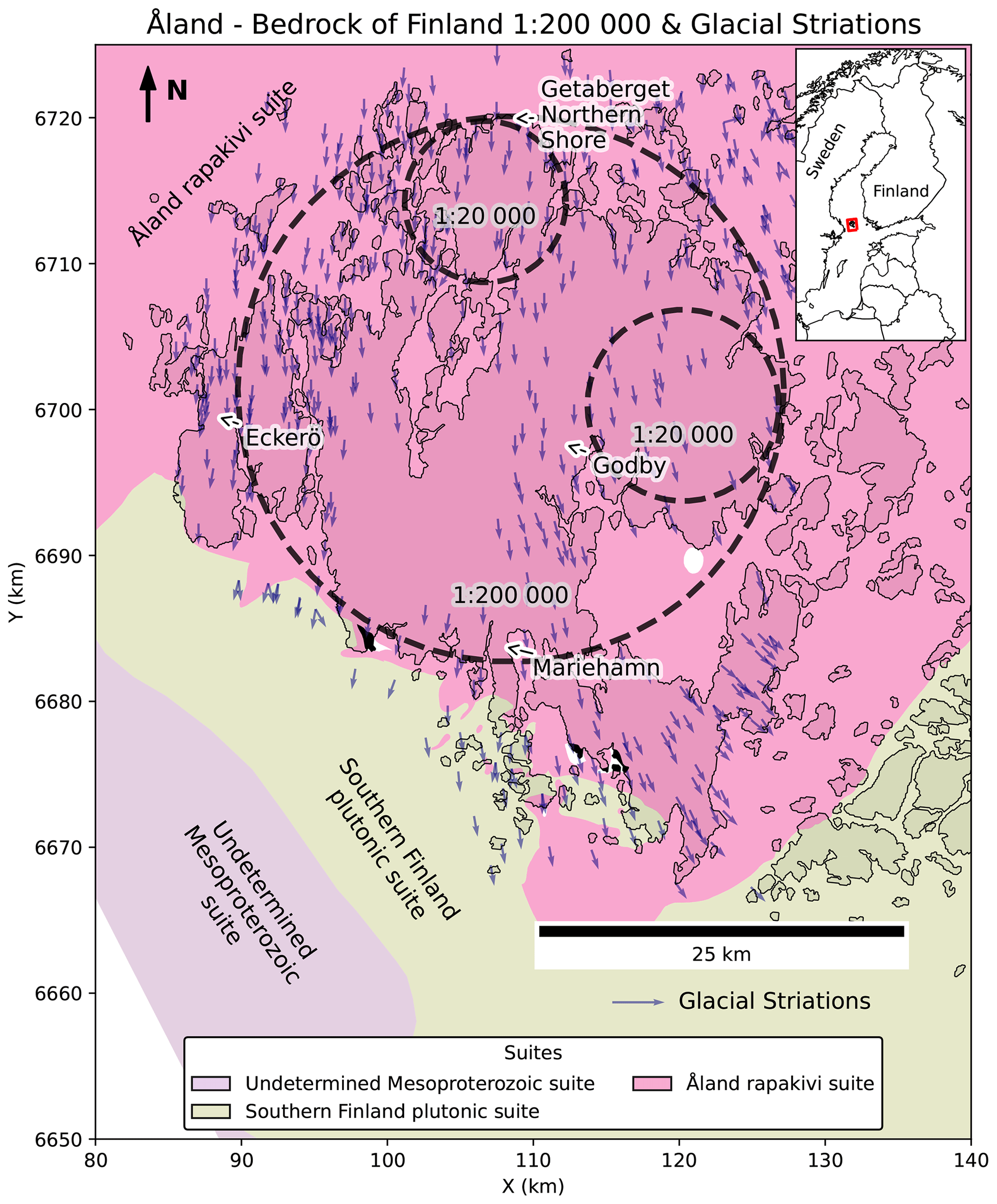
Figure 1 Lithological suites (Geological Survey of Finland, 2017), target areas for lineament extraction (1:200 000 covers most of the main island, while 1:20 000 areas only cover the northern and eastern parts) and glacial striations mapped by the Geological Survey of Finland (Geological Survey of Finland, 2014).

The topography and quaternary deposits on the Åland Islands are shaped by several glaciation cycles during the Pleistocene. Glacial striations (Fig. 1) and distinct glacial landforms such as flutings, typically visible in digital elevation models (e.g. Ojala and Sarala, 2017), indicate that the glacier moved in approximately N–S directions during the latest glacial periods. Besides the smooth-abrasion-related glacial erosion (see above), the fracture systems within the bedrock contributed towards glacial quarrying, which was particularly intense within individual larger faults (Skyttä et al., 2023).

3 Data & methods

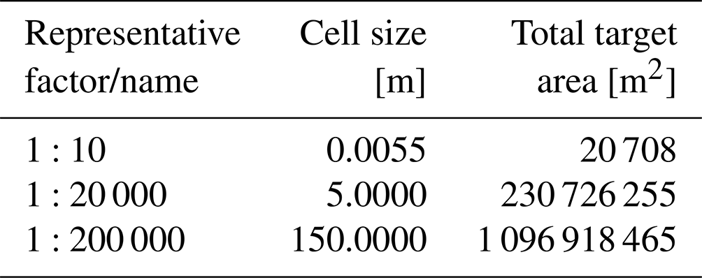
We identify the different scales of observation used for fracture and lineament interpretation by the representative factor, i.e. the ratio between a distance on a map and the distance on the ground (Goodchild, 2011). As an example, 1:10 states that 1 m on the map represents 10 m in nature. However, the representative factor used for representing the scale of digital data displayed on a computer screen is not well defined. This is due to various factors, such as differences in software and display hardware (Goodchild, 2011). To better specify the scale of observation, the use of areal extent and resolution of data are preferred (Goodchild, 2011, 2001), and we display these characteristics in Table 1, with resolution given as the cell size of the raster and the areal extent given as the total target area. The used representative factors should only be considered to be a convenient naming schema, as the resolution better defines the scale of observation. Generation of traces at all the involved scales is conducted remotely from aerial datasets, which allows comparisons between the well-represented sub-vertical features, while the sub-horizontal ones are underrepresented and hence not further discussed in this paper.

Table 1 Definitions of scales of observation used in this study. The name of each scale comes from the representative factor that roughly represents the resolution of the raster used as the base map. The resolution of each named scale is given as the cell size of the raster. Areal extent is given as the total target area of the target areas used in the digitisation of fractures or the interpretation of lineaments.

3.1 Data

Brittle bedrock discontinuities can be classified based on several characteristics, including fracture filling, kinematics and geometry, resulting in a number of terms that can be used to refer to the different types (e.g. joint, vein, fault and fracture; Odling et al., 1999). We use the most general term fracture when referring to brittle discontinuities in general, as we do not discriminate between different types in the analysis. Categorisation of the outcrop fractures digitised from orthomosaics could be done in the field, but to gather representative data on circa 40 000 fractures would require significant resource and time investment. In addition, the results would be difficult to integrate with the remotely digitised data, as the scale of observation would likely be different. Furthermore, field verification of lineaments is much more difficult due to quaternary cover and preferential erosion of the depressions. We consequently attempt to analyse the data without specific prior knowledge of the types of features the fractures and lineaments represent. We refer to the networks of both fractures and lineaments as fracture networks and use it as a general term for the collections of fracture or lineament traces.

We used existing fracture trace data published by Ovaskainen et al. (2022) from the northern shore of the Åland Islands as the outcrop-scale 1:10 dataset (Fig. 2). The data contain fractures with lengths from centimetres to roughly 30 m. The available trace data were originally digitised from orthomosaics spanning an area of circa 20 700 m² using 13 circular two-dimensional target areas along the E–W-trending Getaberget shoreline. The circle diameters ranged from 20 to 50 m, and the number of digitised traces within the circles varied from 358 to 7319. The dataset requires no modifications for the purposes of this study. However, rather than investigating each target area individually, we merge the trace data (n=42 499) into a single dataset of traces that are cropped specifically to the associated target areas, resulting in a trace count of 41 544. There are significant variations in fracture network properties between the target areas but without apparent spatial trends that could be used to correlate the characteristics with their location (Ovaskainen et al., 2022). Therefore, the merging of the data produces an aggregated dataset of the fracture characteristics, representative for the entire Getaberget shoreline study area.

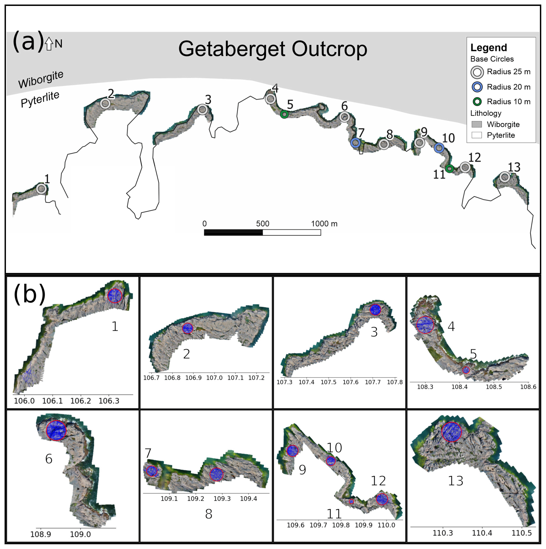
Figure 2 (a) Overview of the Getaberget outcrop with local lithology (Geological Survey of Finland, 2017). Figure from Ovaskainen et al. (2022). (b) Drone-imaged orthomosaics superpositioned with fracture digitisation target areas and digitised fracture traces. Data from Ovaskainen et al. (2022).

Lineaments in this paper are defined as sub-linear lines on the surface of the Earth (see e.g. Tyrén, 2011; Nur, 1982) which are visible in one or more datasets, such as in a digital elevation model or in a geophysical raster. All lineaments digitised for this paper are interpreted remotely by three operators working collaboratively, and cross-verification of interpretations between operators was done to try to minimise subjective bias (see e.g. Andrews et al., 2019; Bond et al., 2007, for further discussion on subjective biases). The lineaments have not been geologically verified in the field. We used the publicly available airborne light detection and ranging (lidar) point data published by the National Land Survey of Finland (2010) to create a digital elevation model (DEM) for the purposes of lineament interpretation in the 1:200 000 and 1:20 000 scales. The used point data have a point cloud density of 0.5 points m⁻², and the mean altitude error is 0.3 m. Specifically, a cell size of 150 m is used for the 1:200 000 scale, and a cell size of 5 m is used for the 1:20 000 scale interpretation. We visualise the DEM using a multi-directional oblique hillshade on top of the DEM raster to highlight the topographical valleys and slopes (Palmu et al., 2015). The hillshade has a z factor of 1, the used altitude of light is 45^∘, and the illumination azimuths are 225, 270, 315 and 360 in degrees. We overlaid the transparent (alpha value 0.3) white-to-black hillshade upon the blue-to-red DEM raster to allow the optimal recognition of linear structures with variable trends. Furthermore, we calculated the colour scales of both rasters from the current extent of the canvas; i.e. the colouring is recalculated dynamically as the interpreter pans or zooms the map. In the 1:20 000 scale, we interpreted topographical lineaments from target areas of ca. 231 km².

In addition to the lidar DEM topographical raster, we interpreted geophysical lineaments in the 1:200 000 scale using regional low-altitude magnetic and electromagnetic aerogeophysical rasters (Hautaniemi et al., 2005). The flight altitude and flight line spacing during the acquisition of magnetic data were 30 and 200 m, respectively, and the acquired raw data were further processed into various rasters with a 50 m cell size. We resampled all the geophysical rasters we used for the 1:200 000 scale interpretation to a cell size of 150 m to match the resolution of the resampled 1:200 000-scale lidar DEM. The target area for the 1:200 000 lineament interpretation covers an area of ca. 1097 km².

We used the following three magnetic rasters: (i) total definitive geomagnetic reference field 65 (DGRF-65) greyscale, (ii) sharp-filtered total field DGRF-65 greyscale and (iii) tilt derivative (Verduzco et al., 2004). Based on these three magnetic raster maps, we interpret lineaments along the recognised linear magnetic maxima and minima, which ideally correlate with deformation zones characterised by metamorphically generated magnetite or pyrrhotite or fluid-induced alteration and leeching, respectively (see Paananen and Posiva Oy, 2013; Middleton et al., 2015, and references within both).

We used one electromagnetic raster from the same national surveying programme, a 3 kHz quadrature component greyscale map, which we used to interpret electromagnetic lineaments. Lineaments from this map are interpreted along the local minima which correspond to either (i) electrically conductive brittle damage zones (with water and/or conductive minerals) or (ii) linear topographic depressions caused by the preferential erosion of brittle damage zones and containing conductive soils with clay minerals and peat alongside rainwater (see Paananen and Posiva Oy, 2013; Middleton et al., 2015, and references within both).

After the interpretation of lineaments from each source (the lidar DEM, the magnetic maps and the electromagnetic map), we integrated the lineaments into a single dataset where lineaments interpreted from different sources were merged based on their superposition following (Engström et al., 2023). Overlapping lineaments were merged along the overlapping parts, while the deviating segments such as splays were preserved. This integrated lineament dataset is the representative dataset used for the 1:200 000 scale in all analyses. We use QGIS 3.14 (QGIS Development Team 2020) and ArcMAP 10.6.1 to digitise the lineaments as georeferenced polylines. Similarly to Ovaskainen et al. (2022), we used the snapping functionality present in both software packages in order to honour the true abutment relationship between the traces and consequently to document realistic topological relationships of the network (Nyberg et al., 2018). To verify the topological consistency of the lineaments, the traces are validated with a Python package, fractopo, which provides a validation utility to find e.g. V nodes and overlapping lineament sections (Ovaskainen, 2022). The 1:200 000-scale lineaments were digitised by three persons, including the main author, while the 1:20 000-scale lineaments were digitised solely by the main author. The interpretations were done in circular target areas to remove the uncertainty related to the shape of the interpretation area (Mauldon et al., 2001; Rohrbaugh et al., 2002; Ovaskainen et al., 2022).

3.2 Lineament and fracture network characterisation and comparison

The interpreted lineament dataset is comparable to the used fracture trace data because it has been digitised and validated similarly and is therefore analysable using the same tool used by Ovaskainen et al. (2022), fractopo. All functionality required for the multi-scale analysis of the lineament and fracture trace data of this paper are implemented in the main fractopo software repository (Ovaskainen, 2022). The fractopo software itself is based on a number of open-source Python packages which enable the specialised geospatial analysis and plotting within this paper. Most prominently, matplotlib (Hunter, 2007), geopandas (Jordahl et al., 2022), numpy (Harris et al., 2020), shapely (Gillies et al., 2022) and powerlaw (Alstott et al., 2014) were used. To allow easier reproducibility of the results of this study, including most figures and tables, the methods and associated code are presented in a separate open repository (Ovaskainen, 2023).

For each scale of observation, 1:10, 1:20 000 and 1:200 000, we present a set of network characterisation results. Fracture intensity P21 is calculated from the total trace length that occurs within an area. The derivatives of it, dimensionless intensity P22 and B22, are calculated by multiplying the value of fracture intensity P21 by the characteristic trace or branch length, respectively (Sanderson and Nixon, 2015). As these two derivative parameters have no units (i.e. they are dimensionless), they are well suited for intensity comparisons between scales. We used equal-area length-weighted rose plots to visualise the azimuth distributions (Ovaskainen et al., 2022; Sanderson and Peacock, 2020) and further subdivided them into sets that occur in all or in at least two of the scales. To analyse network topology and to present topological network characteristics, we determined the topological branches and nodes (Manzocchi, 2002; Mäkel, 2007; Sanderson and Nixon, 2015; Nyberg et al., 2018) of the network using fractopo. Nodes represent interactions between traces or trace abutments in isolation. Specifically, Y nodes represent trace abutments to each other, X nodes represent traces cutting through each other, and I nodes represent non-connected nodes (Manzocchi, 2002; Mäkel, 2007; Sanderson and Nixon, 2015). The node types can be generalised to be connected or unconnected where the X and Y nodes are connected (C) and where I nodes are unconnected (I). Using this generalisation, the branches, which are the trace segments between the nodes, can be given types of C–C, C–I and I–I, where the type is determined by the end nodes of each segment (Sanderson and Nixon, 2015). The branches and nodes were analysed for scale-independent estimates of network connectivity by plotting the relative proportions of different types of nodes and branches into ternary plots (Manzocchi, 2002; Sanderson and Nixon, 2015) and by calculating the parameters of connections per trace and connections per branch (Sanderson and Nixon, 2015).

Regarding the fracture and lineament lengths, we determined power-law, lognormal and exponential distribution fits to trace length data using fractopo, which in turn uses the powerlaw package (Alstott et al., 2014) for maximum likelihood estimation of the fits using the probability density function Clauset et al. (2009). Following Bonnet et al. (2001) and Clauset et al. (2009), the power-law-modelled distribution of lengths n(l) is represented as a function of the power-law exponent a and a constant A as follows:

$$\begin{array}{}\text{(1)}& n\left(l\right)=A\times l^a.\end{array}$$

Along with the length distribution fits, the powerlaw package automatically determines the cut-off value for the length data below which lengths do not seemingly fit the same power-law exponent. This truncation cut-off at the tail end of the distribution is attributed to the fixed scale of observation (see e.g. Bonnet et al., 2001; Pickering et al., 1995, for a discussion on the truncation and censoring of sampling issues for fractures). For fracture trace data, the need for a truncation cut-off is attributed to the insufficient ability to digitise the smallest fractures visible in the images due to insufficient resolution (Pickering et al., 1995; Bonnet et al., 2001). To visualise the length distributions, we plotted the lengths on the x axis and the complementary cumulative number of the length distribution on the y axis. Both axes, x and y, are logarithmically scaled. Cumulative number in this study means a running integer number starting from 1 (the shortest fracture), then counting upwards and ending at the longest. The prefix “complementary” means that the cumulative number is then inversed so that the longest fracture has the smallest value. If the data are power-law distributed, the scatter data on the plot will follow a sub-linear trend with an expected deviation from the trend at some cut-off value. We tested the goodness of fit of a power-law trend by comparing the fit to the fit of a lognormal distribution. We display the log-likelihood ratio R and ratio significance p values of the likelihood comparisons (Alstott et al., 2014). The log-likelihood ratio R is positive when the power-law trend is more likely, and it is negative when the lognormal trend is more likely. High statistical significance of the comparison is described by low p values, where a p value of less than 0.1 is considered to be statistically very significant (Clauset et al., 2009). Because the power-law fit typically requires a cut-off when comparing the different distributions, all comparisons are made to the cut-off-truncated (i.e. cut) data rather than to the full-length data to enable the comparison of the fits as recommended by Clauset et al. (2009). Furthermore, we analysed the lengths of the network branches and used the same determination method as used for the traces to fit different potential distributions to the branch length data. The lengths of topological branches are less subject to subjective bias related to the interpreter (Sanderson and Nixon, 2015; Loza Espejel et al., 2020; Sanderson and Nixon, 2018). Consequently, the results of the length distribution analysis of branches are potentially better suited to comparisons between scales of observation in this study or to comparisons to other studies of branch length distributions (Sanderson and Nixon, 2015; Loza Espejel et al., 2020; Sanderson and Nixon, 2018; Lahiri, 2021). In the Appendix, we also display power-law, lognormal and exponential fits to the full-length data for both traces and branches along with their associated statistical characteristics (Fig. B1 and Table B1 in Appendix B, respectively). This analysis is included in the Appendix due to the inability to compare the fits statistically to fits to data with the applied cut-offs. Figure B1 in Appendix B shows that the power law cannot model the lengths without a cut-off for small lengths, as it disproportionately follows the horizontal trend of the tail lengths.

In addition to the truncation effect, our trace data are probably also affected by censoring, i.e. the inability to sample the longest traces due to limited target areas (Bonnet et al., 2001; Pickering et al., 1995). To investigate the effects of censoring on trace length data, we plot the power-law exponent, the truncation cut-off and the total cut-off proportion as a function of censoring cut-offs. The visual inspection of these plots can be used to compare the different scales regarding the effect of censoring. However, these plots cannot be used to statistically determine the censoring cut-off. However, they can provide alternative power-law exponent values for all scales if censoring is interpreted or assumed to affect the data. Although this analysis could be expanded with the addition of lognormal and exponential fit characteristics and comparisons to the power law, further analysis is out of scope of this study, as the power law is the basis for multi-scale length analysis. The effect of censoring on branch lengths has not been widely studied and is probably of less significance than for traces (Sanderson and Nixon, 2015). Thus, it is not examined in this study.

As we had trace length data of structures from multiple scales of observation, we could investigate the potential fractal nature of the lengths by plotting all trace length data onto a single plot and fitting a power-law function to the data (Sornette et al., 1990; Davy, 1993; Bonnet et al., 2001; Davy et al., 2010). We conducted this analysis as there is physical rationale for brittle structure trace lengths to follow power-law distributions across different scales of observation (Bonnet et al., 2001). To normalise the scale of observation we divided the complementary cumulative numbers (CCMs) of each scale dataset by the total area of the target area to get the area-normalised complementary cumulative numbers (ANCCMs) following Bonnet et al. (2001). Rather than using all the trace length data, we used the truncation cut-offs, determined from individual length distributions, to remove the tails (lowest trace lengths) from the distributions before fitting the multi-scale trend. The trace length data might also be affected by censoring, which might skew the multi-scale length distribution. No method is known to the authors that could reproducibly determine both the truncation and censoring cut-offs simultaneously for all scales in multi-scale length analysis. Therefore, we refrained from using a censoring cut-off. We base this decision both on the lack of a reproducible method and due to our fitting procedure using the complementary cumulative number. The use of the cumulative number causes the number of data points to affect the weighting of the fit. Subsequently, the tail lengths would disproportionately affect the trend of the fit due to the high quantity of low lengths compared to the head lengths, which have a negligible effect on the trend. Consequently, using truncation cut-off for the tail lengths is more important than using a censoring cut-off for the head lengths. The truncation cut-offs can also be reproduced, although our procedure only determines them from the single-scale length data. To fit the power-law trend, we could not use the powerlaw package, as it does not support automatic fitting to multiple, separate distributions simultaneously. Rather, we used a least-squares polynomial-fit function, polyfit from the numpy Python package (Harris et al., 2020), and assessed the multi-scale goodness of it with the mean squared logarithmic error (MSLE). The fit is done to the logarithm of the length and ANCCM data, as implemented in fractopo (Ovaskainen, 2022). This is in contrast to using the probability density function, as was done for single-scale length distributions. However, the resulting exponents are still comparable. Using multi-scale azimuth sets determined from a visual inspection of rose plots of the scales of observation, we could further investigate the possibility of fitting multi-scale power-law trends to multi-scale length data that are categorised by azimuth set. The approach has the potential to reveal differences between the length distributions of fractures and lineaments in different azimuths (e.g. Skyttä et al., 2021; Ceccato et al., 2022). Of particular interest is whether the effect of glacial erosion has caused differences in the length distributions of features in different azimuths.

4 Results

4.1 Lineament interpretation

Lineament interpretation and subsequent integration of topographic and geophysical lineaments in the Åland Islands resulted in 201 integrated lineaments in the 1:200 000 scale. The number of lineaments from each different interpretation source in the 1:200 000 scale is displayed in Table 2. The addition of geophysical rasters to complement lidar DEM-based interpretation resulted in a significant number of additional lineaments. Specifically, a significant number of geophysical lineaments with a NW–SE-trending azimuth were added (Fig. 3). The effect of glacial erosion in the N–S direction is apparent in the lidar raster but is not visible in any of the geophysical rasters. Practically, no N–S-oriented lineaments were interpreted from the geophysical rasters, whereas in the lidar raster, a significant number of such lineaments were digitised in the 1:200 000 scale. Lineament digitisation in the scale 1:20 000 was limited to the lidar DEM raster, as the geophysical rasters lacked the resolution for the more accurate extraction possible in the 1:20 000 scale. The digitisation resulted in 609 lineaments, which are visualised in Fig. 4a. The northern target area for 1:20 000 lineament interpretation covers the Getaberget hill area and the surrounding terrain (Fig. 1). Because the hill area is distinctly better exposed than the neighbouring terrain, the interpreted lineament density is higher in this more exposed and elevated area (Fig. 4a)

Table 2 Counts of digitised fractures and lineaments from each source that intersect their respective target areas.

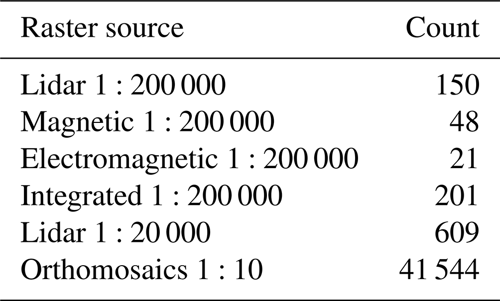
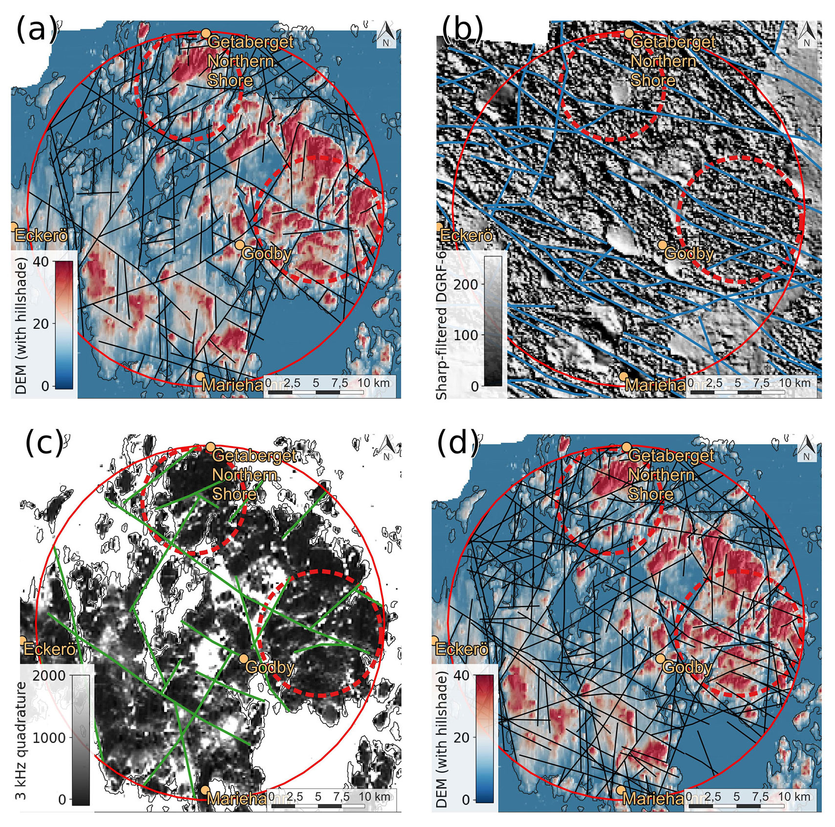
Figure 3 All panels (a–c) contain the 1:200 000-scale lineaments that were interpreted using the displayed raster. In the case of panel (b) two other magnetic maps were used (total field DGRF-65 and tilt derivative DGRF-65) to interpret the displayed lineaments (see Appendix A). (a) Map of a light detection and ranging (lidar)-based digital elevation model (DEM) with a hillshade overlay. (b) Map with greyscale-visualised sharp-filtered DGRF-65 magnetic data. (c) Map with greyscale-visualised 3 kHz quadrature component electromagnetic data. (d) Same map as panel (a) but with the integrated lineaments overlaid on top.

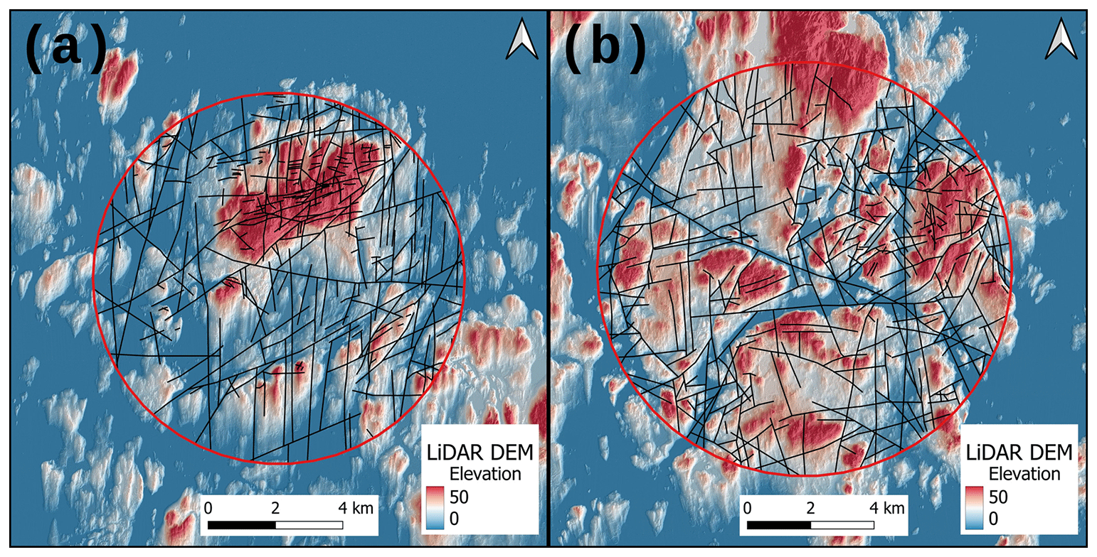
Figure 4 Lidar DEM overlaid with digitised 1:20 000-scale lineaments and the two separate target areas. (a) Northern area of Getaberget. (b) Eastern area near Godby.

4.2 Multi-scale network characterisation

Scalar network characteristics of each scale dataset are collected in Table 3. The characterisation consists of geometric and topological parameters which can be used to compare the scales. Of special interest are the dimensionless parameters (dimensionless intensity P22 and B22, connections per trace, connections per branch, and trace and branch power-law exponents), as these are especially suited for comparisons between scales of observation (Sanderson and Nixon, 2015; Goodchild, 2001). The scale-dependent fracture intensity P21 has an expected trend of higher intensity with higher scale, with the 1:10 scale having the highest value and the 1:200 000 scale having the lowest. The trend is opposite for dimensionless intensity B22, with the 1:200 000 scale having the lowest value. Connections per trace and connections per branch display a trend with values decreasing as the scale increases, with the 1:10 scale having the lowest value. While the values of connections per branch are quite similar for the 1:20 000 and 1:200 000 scales (1.75 and 1.85, respectively), the difference is amplified by the limited range of values for connections per branch (0.0–2.0; Sanderson and Nixon, 2015).

Table 3 Basic network descriptions of all scales of observation, with units displayed when applicable. EM – electromagnetic 3 kHz quadrature. Mag – magnetic rasters.

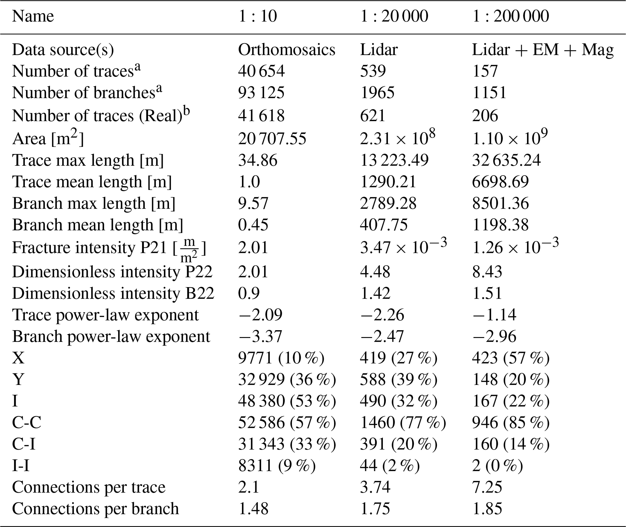
^a Based on node counting (Sanderson and Nixon, 2015). ^b The absolute (i.e. the real) count of trace geometries.

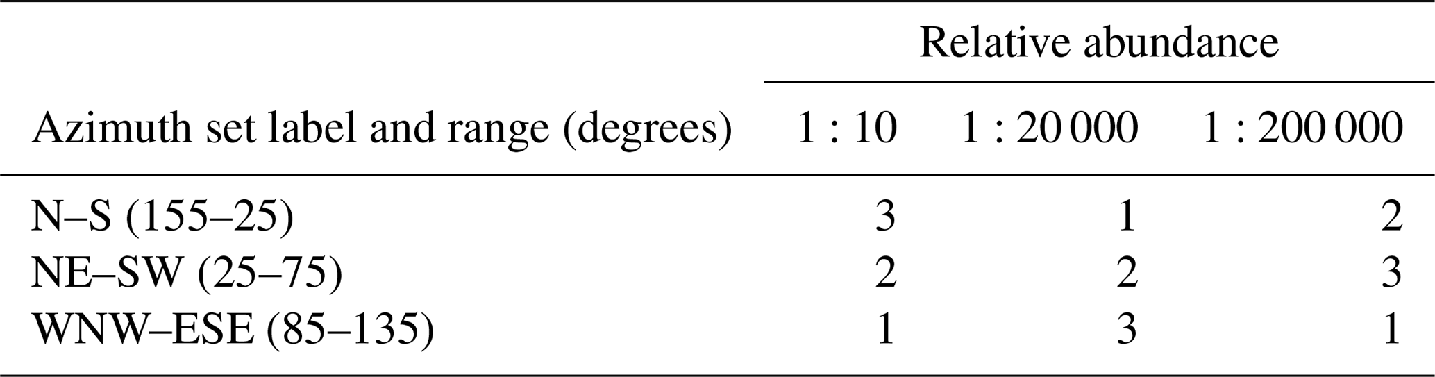
The individual azimuth and length analysis results for each scale are visualised in Fig. 5, where trace azimuths are represented with equal-area length-weighted rose plots (Sanderson and Peacock, 2020) and where trace and branch lengths are modelled with power-law, lognormal and exponential fits. Based on the displayed rose plots (Fig. 5a), three distinct azimuth sets occur in all scale datasets (Table 4). The sets occur with different intensities in different scales, which is recorded in Table 4 with the following numbering: 1 equals the most abundant set, and 3 equals the least abundant set. Relative abundance is based on the displayed percentages of the total trace length of each set in Fig. 5a. The relative abundance of the sets differs greatly between the scales, and when the set is labelled as the least abundant (3), the occurrence of it in the scale is vague. For example, the N–S set is barely visible in the 1:10-scale rose plot (Fig. 5a), with only a minor local maximum detectable at around 175^∘. Similarly, the WNW–ESE set is barely detectable in the 1:20 000-scale rose plot without any detectable local maximum.

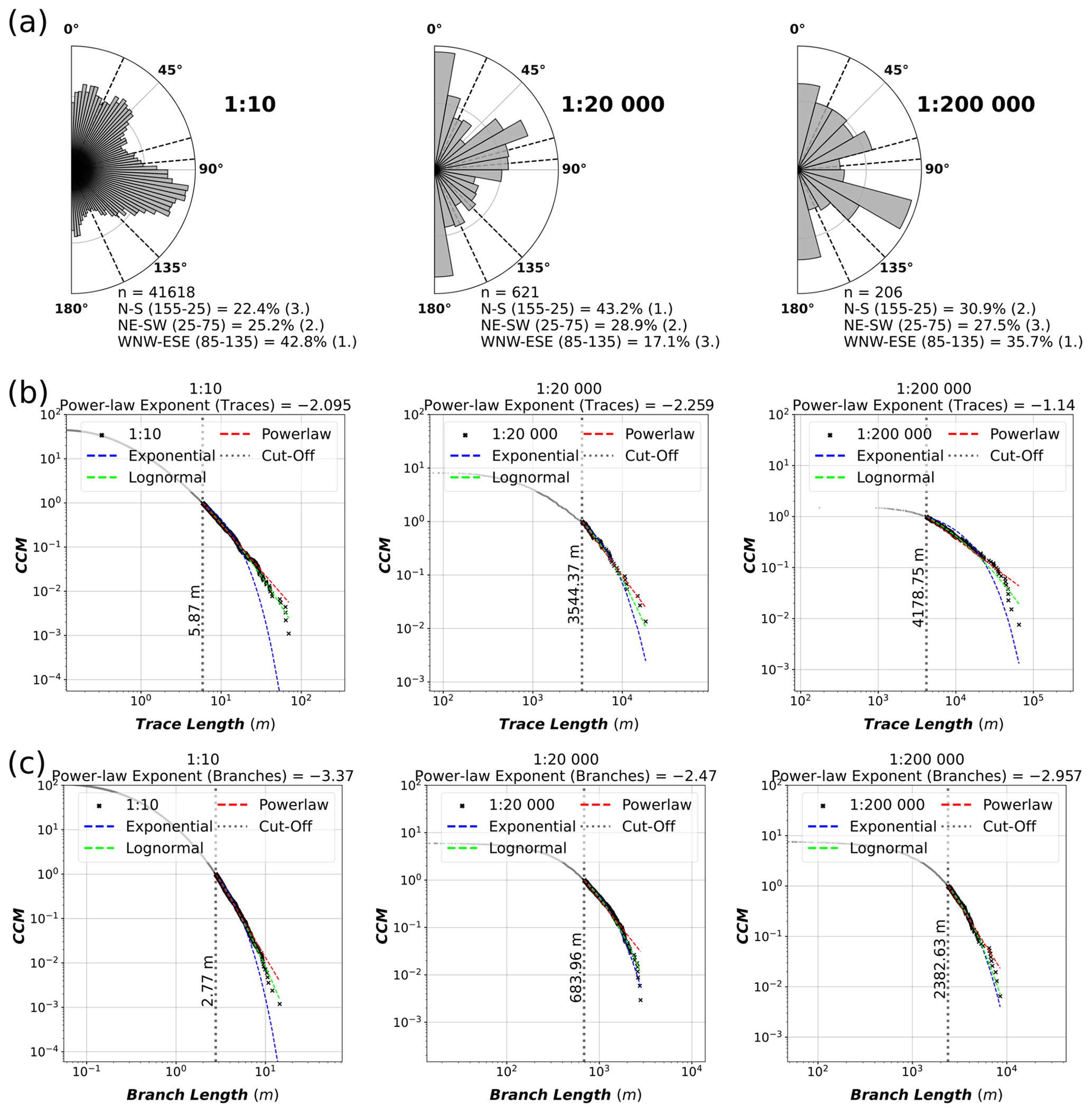
Figure 5 (a) Equal-area length-weighted rose plots of trace azimuths of each scale along with the percentage of the total length that each set contains. The determined sets do not cover all azimuths, and therefore, the percentages do not add up to 100 %. (b) Length distributions of traces of each scale on plots with complementary cumulative number (CCM) on the y axis and trace length on the x axis. The distributions are fitted with power-law, lognormal and exponential fits, and the automatically determined power-law truncation cut-off is indicated with the vertical dashed line and text. (c) Length distributions of branches with the same setup as subfigure (b), except for the x axis, which has branch lengths rather than trace lengths.

Table 4 Visually determined multi-scale trace azimuth sets along with the relative abundance in each scale, where 1 equals the most abundant of the sets and equals 3 the least abundant.

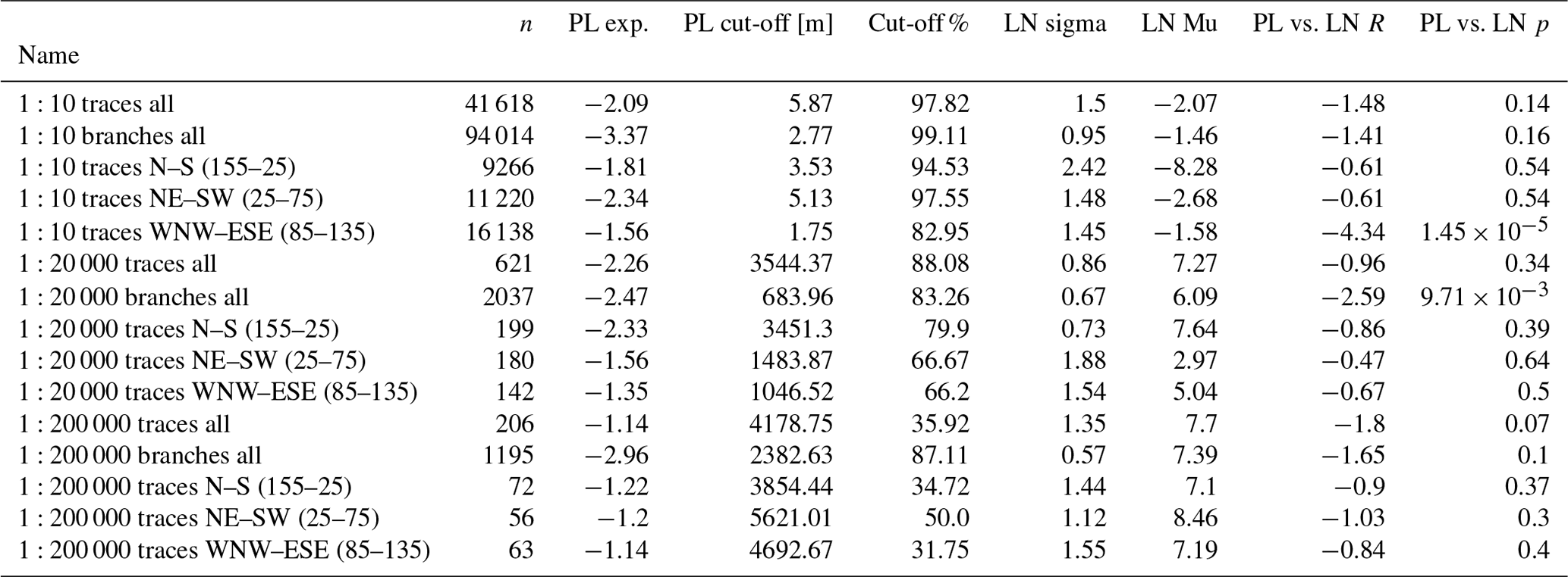
The exponents of the fitted power-law trends for trace lengths vary drastically when comparing fractures and lineament scales: the 1:10- and 1:20 000-scale fracture traces have fitted trace power-law exponents of −2.095 and −2.259, respectively, whereas the 1:200 000 traces have an exponent of −1.14 (Fig. 5b). However, 1:10- and 1:200 000-scale branch lengths have relatively similar exponents of −3.37 and −2.96, respectively, whereas the 1:20 000-scale branch lengths have an exponent of −2.47. Further characterisation of the trace length distributions is displayed in Table 5, where the power-law fit is compared to the lognormal fit (see rows with “All”) and the cut-off proportions are displayed. Comparisons to exponential fits are not displayed, as even visual inspection shows that it does not model the cut length distributions well (Fig. 5b). For all scales, the lognormal fit is more probable according to the R values. However, based on the p values, the lognormal fit is significantly more probable than the power-law fit for the 1:200 000 scale (p value less than 0.1), while the power law remains a possible alternative for both the 1:10- and 1:20 000-scale datasets. The cut-off proportion (i.e. the amount of data removed by the application of the cut-off) for the 1:10 scale is very high, with 97.82 % of data being cut off. The proportion is similarly high for the 1:20 000 traces, with a value of 88.08 %, and is significantly lower for the 1:200 000 traces, with a value of 35.92 %.

Table 5 also contains fit results to azimuth set-wise-categorised trace lengths for each scale. For all scales, the set-wise fits do not drastically differ from the fits to all traces in terms of power-law exponents. The power-law fits for 1:10-scale azimuth set lengths remain candidate fits, expect for the WNW–ESE set, where the lognormal fit is significantly more probable with a p value of $\mathrm{1.45}\times {\mathrm{10}}^{-\mathrm{5}}$. For both the 1:20 000 and 1:200 000 scales, all azimuth set-wise fits have p values of over 0.1, indicating that the power-law fit cannot be ruled out as a candidate model for the trace lengths of each set. However, for these comparisons, it should be kept in mind that the azimuth sets occur with very different intensities across the scales of observation (Table 4). Furthermore, as the traces are subdivided into sets, the sample count within each set decreases, which lowers the reliability of the results, especially for the 1:200 000-scale lineaments (Table 4). Regardless of these uncertainties, a common trend is noticeable where the WNW–ESE set traces have the highest power-law exponents in all scales.

Table 5 Parameters of length distribution fits for traces and branches for all scales, along with set-wise fits of traces for all scales. PL – power law. LN – lognormal. The R value is the log-likelihood ratio, where a positive value indicates that the power-law fit is more likely and a negative value indicates that the lognormal fit is more likely. The p value represents the significance of the likelihood where low values (<0.1) correspond to high statistical significance.

The effect of censoring on individual-scale trace data is visualised in Fig. 6, where the power-law exponent (Fig. 6a, d and g), cut-off (Fig. 6b, e and h) and cut-off proportion (Fig. 6c, f and i) are plotted as a function of censoring cut-offs ranging from the minimum trace length to the maximum. For 1:10-scale fracture trace data, the application of a censoring cut-off of approximately 25 m seems to cause the automatic truncation cut-off determination to dramatically lower the truncation cut-off and simultaneously decrease the proportion of data that is removed by the cut-offs for the power-law fit from the original proportion of circa 98 % (Table 5) to circa 84 % (Fig. 6b and c). Simultaneously, the power-law exponent increases to a value in the range of −1.6 to −1.5 (Fig. 6a). For the 1:20 000-scale data, the cut-off proportion is dramatically lower (circa 62 %), with a censoring cut-off of circa 10 000 m, but the proportion then increases as the censoring cut-off is lowered more (Fig. 6f). The trends for 1:20 000-scale data have similarities with the 1:10 data, as the exponent with the censoring cut-off of circa 10 000 m is also in the range of −1.6 to −1.5 (Fig. 6d). Both 1:10 and 1:20 000 results are in contrast to the 1:200 000-scale data, where the application of a censoring cut-off somewhat consistently increases the proportion of data removed by the cut-offs in power-law fitting (Fig. 6i) and decreases the value of the power-law exponent (Fig. 6g).

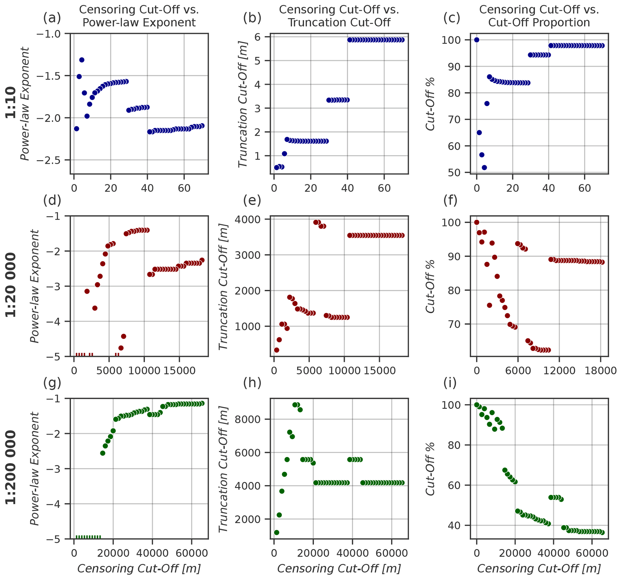
Figure 6 Plots of power-law characteristics as a function of a range of censoring cut-offs from the maximum trace length to the minimum. The relationships are shown for the trace lengths of the three scales. (a, d, g) Power-law exponent as a function of censoring cut-offs. Exponents below −5.0 are included as ticks at the bottom of the plot. (b, e, h) Automatically determined power-law truncation cut-off as a function of censoring cut-offs. (c, f, i) The total proportion of data cut-off by both censoring and truncation cut-offs as percents as a function of censoring cut-offs.

The multi-scale power-law fit to all traces is visualised in Fig. 7a along with fits to trace lengths categorised by the previously determined azimuth sets in Fig. 7b–c. Based on visual inspection of the plot with all trace data (Fig. 7a), the 1:10-scale fractures and the 1:200 000-scale lineaments seem to follow a common power-law trend, while the 1:20 000 lineaments deviate from it. However, the tail cut-offs majorly affect the distributions and the resulting fits. Also, the largest length traces (head) within each scale deviate from the common trend. When comparing the azimuth set-categorised multi-scale length distributions (Fig. 7b and c), the WNW–ESE set is somewhat anomalous compared to the rest. Due to having lower cut-offs, determined from individual distributions (Table 5), a higher proportion of length data is used with the WNW–ESE data, which increases the mean squared logarithmic error (MSLE), but, based on visual inspection, a common trend seems more likely for 1:10-scale fractures with intermediate lengths (length data around the cut-off value of 1.75 m) rather than the higher-length fractures at the head of the distribution (Fig. 7d). The exponent values of the power-law trends are quite similar across the different arrangements (Fig. 7). The NE–SW set has the highest exponent of −1.12, closely followed by the exponent of all traces (Fig. 7a–d) and the exponent of the N–S set trace lengths (−1.19). The WNW–ESE-trending traces have the lowest exponent of −1.30, which deviates slightly from the other exponents (Fig. 7d) and is in contrast to the set having the highest exponents when analysing the length distributions individually (Table 5). The trend of the individual 1:10 fracture and 1:20 000 lineament distributions in Fig. 7a and b seems to indicate a power-law exponent lower than the trends of the lineaments, as is also evidenced by fits to the individual distributions where the exponent is −2.095 for the 1:10-scale fractures and −2.26 for the 1:20 000-scale lineaments (Fig. 5).

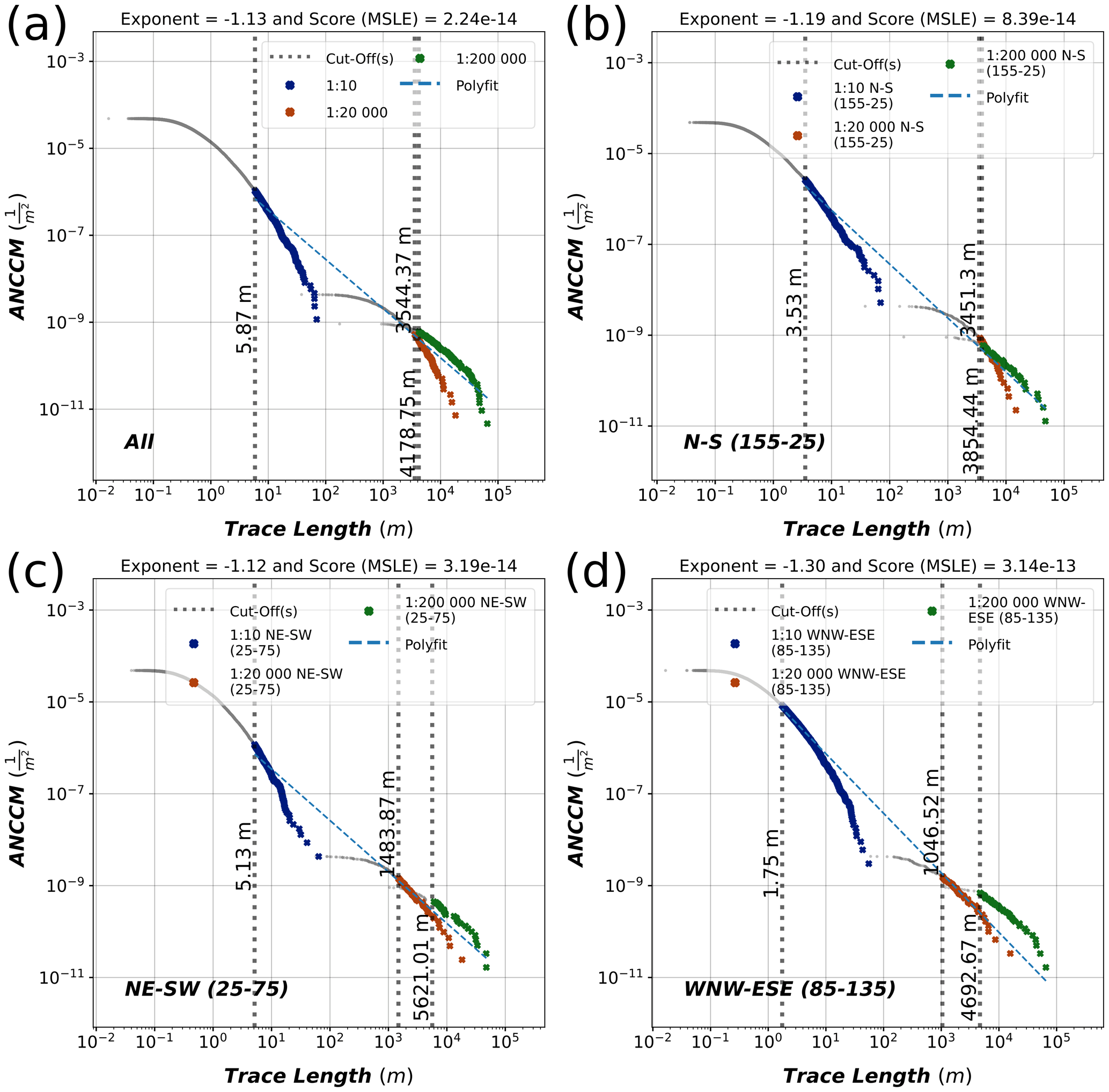
Figure 7 Plots of multi-scale length distributions with similar plot arrangement to panels (b) and (c) of Fig. 5. However, instead of complementary cumulative number, we use the area-normalised complementary cumulative number (ANCCM). The goodness of fit is estimated using the mean squared logarithmic error (MSLE). The fit is done on the part of the trace length data that is above the truncation cut-off determined from each individual scale (Fig. 5b; Table 5). (a) Multi-scale power-law fit to all trace length data. (b–d) Fits to trace length data categorised by defined azimuth sets (Table 4).

The proportions of topological node types (X, Y and I) and branch types (C–C, C–I and I-I) from Table 3 are visualised in Fig. 8 with ternary plots (Manzocchi, 2002; Mäkel, 2007; Sanderson and Nixon, 2015). From both the node ternary plot (Fig. 8a) and the branch ternary plot (Fig. 8b), a trend can be observed where the apparent connectivity of the network increases as the scale of observation becomes smaller; i.e. the resolution used for interpretation is poorer. Specifically, both the proportion of X nodes and C–C branches increases as the scale becomes smaller, and this is the highest for the 1:200 000-scale network. The trend is also observable from the values of connections per branch and connections per trace (Table 3).

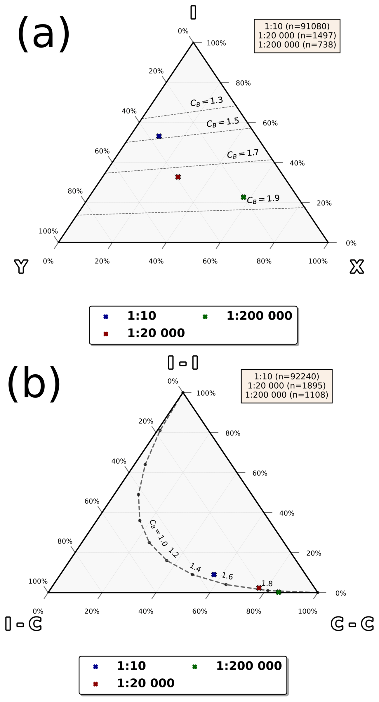
Figure 8 (a) Ternary plot of topological XYI node proportions for each scale. (b) Ternary plot of topological (C–C, C–I and I–I) branch proportions.

5 Discussion

5.1 Gap between outcrop and lineament data

Our use of the 1:20 000 scale of observation in digitising topographical lineaments has the potential to reduce the uncertainty related to the brittle structures of intermediate length (100–500 m) which are commonly missing from studies based on outcrop digitisation and lineament interpretations (Marrett et al., 1999; Strijker et al., 2012; Loza Espejel et al., 2020; Fox et al., 2012). These missing length data were found to be a problem during the creation of a DFN model for the Olkiluoto spent-fuel-disposal facility where fracture or lineament data could not be empirically collected with these lengths (Fox et al., 2012). The DFN model required the creation of fractures of all sizes using a common scaling law (or laws), including ones in this missing length range. Without empirically detected fractures within this size range, an uncertainty remained regarding the validity of generating fractures of these sizes. The generation was done using a length distribution model derived from outcrop fracture data or alternatively from lineament data (or both). All three options required the extrapolation or interpolation into the unknown intermediate length range (Fox et al., 2012). In our study, although we produce lineament length data in the 100–500 m length range (Fig. 5b), the optimisation of the power-law fit to all of the 1:20 000-scale length data resulted in a truncation cut-off of 3544 m (Fig. 5; Table 5). With the use of a censoring cut-off of 10 000 m that was visually optimised for the lowest cut-off proportion, the truncation cut-off could be lowered to circa 1300 m (Fig. 6e and f). These cut-offs, 3544 and circa 1300 m, can be estimated to be the lowest length lineaments which we can consistently interpret without truncation effects caused by the resolution of the lidar DEM in this scale when assuming that the lineament trace lengths follow a power law without or with taking into account the possible censoring of lengths, respectively. In the statistical comparison between the lognormal and power-law fits to the 1:20 000 length data, the lognormal is favoured (Table 5), but the power law is not ruled out due to the p value being above 0.1. If this assumption is challenged and lineaments are assumed to instead follow scale-dependent distributions, such as the lognormal, the problem of missing data in the 100–500 m length range is solved. However, all possibility to interpolate length distributions to any other gaps is ruled out, as the interpolation depends on the lengths following a scale-independent distribution, such as the power law. Consequently, uncertainty remains around the length data gap between the 1:10 outcrop scale and the 1:20 000-scale lineament scale (Fig. 5). The resolution of the lidar DEM could enable the interpretation of lineaments within this length gap by using a larger scale of observation (e.g. 1:10 000). However, in the vast majority of the 1:20 000 area, based on visual observation of the lidar DEM (Figs. 3 and 4), the landforms would become less sub-linear and more uncertain with regard to whether or not they reflect the structures of the underlying bedrock. In contrast, where quaternary deposits do not overlay the bedrock, such as at the Getaberget shoreline outcrops, the bedrock features are directly observable from the DEM. These areas are, however, limited when considering both their shape and areal extent and are better surveyed with drone photography, as the photos have a significantly higher resolution than the DEM. An alternative to drone photography is the use of satellite images (e.g. Bertrand et al., 2015; Mercuri et al., 2023). However, they generally have lower resolution than drone images and do not provide any penetration through vegetation, which limits the area in which they are useful to the same area as the drone images. Digitisation of fractures longer than the diameter of the circular target areas used at Getaberget (50 m) could be possible, but they could not be sampled using circular target areas, as the width of the polished part of the outcrops is limited to not much higher than the diameter of 50 m (Ovaskainen et al., 2022). Using non-circular, irregularly shaped target areas would add uncertainty to the orientation distributions we sample from the target area, which would consequently decrease the significance of the results (Mauldon et al., 2001; Rohrbaugh et al., 2002; Ovaskainen et al., 2022). This limits the use of creating lower-resolution drone images for the purpose of creating lower-scale interpretations from the same drone-imaged areas as we have done with the lidar lineament interpretations where we used resampled resolutions of 5 and 150 m. We could digitise traces from scales such as 1:20, but the maximum length of fracture traces would still be limited to roughly 50 m regardless of the image data used as the source (drone or satellite).

5.2 Factors affecting analysis

A distinct difference in the data between the three scales is the significantly higher number of traces within the 1:10 scale compared to either of the lineament trace datasets (Table 3). Previous studies on the representative trace count required for trace length distribution analysis have suggested minimum trace counts of 150 to 300 (Priest, 1993) and below (Bonnet et al., 2001; Zeeb et al., 2013). The 1:200 000-scale lineament trace count of 201 (Table 5) is lower than the upper threshold by (Priest, 1993) but is higher than the minimum recommendations of 200 and 110 by Bonnet et al. (2001) and Zeeb et al. (2013), respectively. The study by Ovaskainen et al. (2022) on the Getaberget trace dataset, which we use as the 1:10-scale data, suggested that the sample area (and simultaneously, the trace count) could be significantly reduced to still result in the same characterisation results for the Getaberget area. But we cannot rule out the possible effect of low lineament trace counts on the analysis of trace lengths for the 1:200 000 scale. The effect of lower counts of lineaments might also cause the subjective bias related to the interpreters of the lineaments to have more effect, as each individual choice in the lineament interpretation has more weight.

The lineament interpretation in scale 1:20 000 is solely based on the lidar DEM, whereas interpretation in scale 1:200 000 uses geophysical rasters in addition to the DEM to enhance the detection of bedrock structures. This could cause the interpreted structures to differ between the scales, where the structures with high geophysical but low topographical signals would be more likely to be detected in the 1:200 000-scale interpretation. This could explain the lack of a detectable WNW–ESE set in the 1:20 000-scale lineaments (Fig. 5; Table 4), which is detected in the geophysical rasters (albeit as mostly NW–SE-trending lineaments) in the 1:200 000 scale (Fig. 3) and corresponds, azimuth-wise, to the major South Finland shear zone (SFSZ) that seemingly abuts next to the main Åland island (Torvela et al., 2008). The WNW–ESE set is represented by a single long lineament that cuts through the entire eastern 1:20 000 target area (Fig. 3b). However, because it cuts the target area from both ends, it is removed from any further analysis due to the boundary-weighting methodology implemented in fractopo (Fig. 5 by Ovaskainen et al., 2022). The set is otherwise represented by only very few small lineaments (Fig. 5a) The similar azimuth trend compared to that of the SFSZ could indicate that the structures of the Åland rapakivi batholith might inherit a structural trend from the SFSZ, which would, consequently, increase the geological significance of the WNW–ESE-oriented lineaments. The set is more detectable in the 1:10-scale fracture traces, of which some correspond to field-surveyed faults (Skyttä et al., 2023; Ovaskainen et al., 2022). Based on these observations, we suspect that the lack of geophysical data in the 1:20 000 scale could result in a lack of structures that have relatively low topographical signals in that scale, with only the largest WNW–ESE structures being detectable (Fig. 4b). Consequently, we recommend the supplementation of the 1:20 000-scale interpretation with high-resolution geophysical data, as it would increase the certainty of lineament interpretation in that scale. These uncertainties limit the possibility of using the full resolution of the lidar DEM to map lineaments with intermediary lengths (100–500 m; continued discussion from Sect. 5.1). However, geological differences in the quaternary cover and glacial erosion might make the use of the 1:20 000 scale more successful in other study areas and other geological bedrock settings.

The bedrock within the 1:200 000-scale target area lacks precursor fabrics caused by tectonic deformation, as the batholith was emplaced after the Svecofennian orogeny (Rämö and Haapala, 2005). Consequently, we do not expect the fracture or lineament pattern to be controlled by local ductile anisotropies, such as foliations and folds. This simplifies the multi-scale analysis of the fractures and lineaments, as investigating the controlling effect of such structures is not required. We do not expect the 1:10-scale fracture lengths to be strata bound, as the lithology is homogeneous crystalline rock within the entire 1:200 000-scale target area (Fig. 1). However, we cannot have the same expectation for lineaments, especially digitised in the 1:200 000 scale, as their interpreted lengths can span tens of kilometres (Table 3) and they are therefore comparable in size to the sheet-like bodies of rapakivi granite with estimated thicknesses of circa 5–10 km (Rämö and Haapala, 2005). The possible partly strata-bound nature of lineaments might be noticeable in their length distributions, where the lognormal distribution fit to the 1:200 000-scale trace length distribution is better, with a p value of less than 0.1 in the comparison of power-law and lognormal fits indicating high statistical significance of the lognormal preference (Table 5; Fig. 3).

We expect that the digitised lineaments which are oriented roughly N–S are partly affected by the glacial landforms, e.g. in the form of enhancing their length, as discussed in a similar study by Ovaskainen (2020). The N–S-oriented lineaments are, based on visual observation of Figs. 3a and 4, quite continuous, and the effect of glacial erosion is apparent from the lidar raster maps in the form of visible linear quaternary land features such as possible roches moutonnées. Inspection of the length distributions of the N–S-oriented lineaments using power-law modelling (Table 5) shows that the N–S-striking lineaments have the lowest exponents compared to other sets or to all lineaments within both the 1:20 000 and 1:200 000 scales, with values of −2.33 and −1.22, respectively. However, the difference is small compared to other sets for the 1:200 000 scale, and the sample counts of lengths within each set are low enough to possibly affect the reliability of the results. Some evidence of a bedrock-related nature of N–S-trending lineaments is present as local fracture azimuth maxima in individual Getaberget target areas and in previously surveyed fault data (Figs. 6 and 9 by Ovaskainen et al., 2022). In contrast, there is a lack of a dominant N–S set of fractures in the aggregated Getaberget trace data (Fig. 5a; Table 4) The N–S trend is not visible in the geophysical magnetic or electromagnetic rasters either (Fig. 3b and c). In conclusion, through our multi-scale cross-validation, the inclusion of the N–S-striking lineament characteristics in e.g. DFN modelling should be done with caution, and the verification of the existence of N–S-striking bedrock structures should be done in further studies. However, the existence of dextral faults trending N–S (Fig. 9 by Ovaskainen et al., 2022) provides some evidence of N–S-striking bedrock structures.

5.3 Multi-scale analysis

Within all panels of Fig. 7, the length distributions seem to follow the trend of the fitted power law to some degree, although both the slope and location (below or above the power-law trend) of individual distributions vary. The differences in slope compared to the fitted multi-scale power law can be explained for the 1:10 and 1:20 000 scales by the individual power-law exponents of circa −2.0 that deviate clearly from the 1:200 000-scale exponents of circa −1.2. The difference in location could indicate problems with the normalisation of the trace length distributions in the multi-scale plot. On closer inspection of the 1:10 length distributions in Fig. 7, the trend that has been fitted to the lineament trace lengths could fit the centre part (which has lengths below the cut-off) of the 1:10 length distributions. If the cut-off was around 1 m, that part would be included in the fitting, and the trend would have a better continuation, at least visually. However, the head (highest length traces) of the 1:10 distribution would still not fit the multi-scale power law, possibly indicating the need for both a tail (i.e. truncation) and a head i.e. (censoring cut-off). The heads of both 1:20 000- and 1:200 000-scale distributions similarly deviate from the trend. Using a censoring cut-off of circa 25 m for 1:10 fracture trace data would result in an exponent of circa −1.6 (Fig. 6a), which is closer to the 1:200 000-scale exponent of −1.14, further showing the possible need for cut-offs at both ends of the distribution. The use of a global optimisation algorithm that considers all distributions and chooses cut-offs, possibly for both head and tail, to fit a single multi-scale power-law trend rather than determining only the tail-end cut-off from the individual length distributions could majorly improve the process while still allowing the full reproducibility of the fitting process. However, the option also remains that the fractures and lineaments have scaling properties that correlate with the scale of observation rather than having common ones (Kruhl, 2013; Davy et al., 2010). The possibility of using normalisation methods other than area normalisation should also be simultaneously investigated (Bonnet et al., 2001), and the use of the probability density function in place of the complementary cumulative number might have more merit when analysing multi-scale length data (Bour et al., 2002). The occurrence of partly scale-independent azimuth sets (Fig. 5; Table 4) within our data might be indicators of hierarchical organisation of the fracture network, where the different sets cause differences in the scaling laws between scales of observation, similarly to a study by Ceccato et al. (2022), where this option was discussed for their multi-scale fracture and lineament dataset with scale-variant azimuth sets.

The topological characteristics of the multiple scales follow a set trend where the connections-per-branch values decrease when the scale increases from 1:200 000 to 1:10 (Fig. 8; Table 3). A very similar trend was observed in a multi-scale study done in the Loviisa region, southeast Finland, within a crystalline rapakivi batholith (Ovaskainen, 2020). The trend could be the result of e.g. source raster differences (Nixon et al., 2012) or possible differences in the actual topological characteristics between fractures and lineaments of different scales. Another option related to the raster differences is the possible difficulty or subjective bias in identifying two Y nodes in cases where they are close to each other and instead labelling the intersection as a single X node (Andrews et al., 2019). In any case, the possibility of this kind of trend should be kept in mind when determining topological characteristics from only a single scale of observation, as the value might only represent features within that observation scale. This has implications for DFN modelling if topological characteristics are included as input parameters (Libby et al., 2019). Based on the high proportion of X nodes for the 1:200 000-scale lineaments, the connectivity of the fracture network would be estimated to be higher than the estimated connectivity from the 1:10-scale fractures, at least based on this strictly two-dimensional analysis. Future studies could include the estimation of the sub-horizontal fracturing, detected in field surveys (Skyttä et al., 2023), on the connectivity to extend the analysis to the third dimension.

6 Conclusions

• Based on azimuth analysis of our study area, which covers most of the main island of Åland, the regional fracture pattern is dominated by WNW–ESE- and N–S-oriented lineaments. In particular, the WNW–ESE-oriented lineaments can be expected to correspond to large brittle bedrock structures that cut the Åland rapakivi batholith, as they are prominent in geophysical rasters, whereas N–S-trending lineaments might mostly represent glacial deposits rather than bedrock structures.

• Using the scale of observation of 1:20 000, we generated lineament data within the 10 to 500 m interval from which brittle structure data are lacking in past studies. However, the lineament data we collected did not fit a common power-law trend for fractures digitised from the 1:10 scale and lineaments interpreted from the 1:200 000 scale. Further method development on how to address this length gap is therefore still required.

• The length distribution analysis of traces of each scale results in power-law exponents of −2.09, −2.26 and −1.14 for the 1:10, 1:20 000 and 1:200 000 scales, respectively. However, lognormal trends are statistically more likely for all three scales, and the effects of censoring are not taken into account for these values, which causes high uncertainty in whether these power-law exponent results are significant for individual-scale length distributions. A common power-law exponent fitted to all scale length distributions simultaneously has an exponent of −1.13, but the individual distributions might follow distinct power laws better than a common one.

• Investigation of possible censoring of long traces shows that 1:10-scale fracture and 1:20 000-scale lineament traces might be better modelled with a power law when using a censoring cut-off in addition to a truncation cut-off. A power law with an exponent of circa −1.6 was found to fit both scales individually, with censoring cut-offs of circa 25 m and 10 000 m, respectively.

• A trend is observed where the 1:10-scale outcrop fractures show a lower degree of X nodes and values of connections per branch compared to lineaments from scales 1:20 000 and 1:200 000. Furthermore, the 1:200 000-scale lineaments have the highest degree of X nodes and values of connections per branch. This kind of trend in a theoretically scale-independent characteristic should be kept in mind in future studies, especially when restricted to a single scale of observation. The trend might be related to specific methods of digitisation or data rather than natural phenomena.

• The lineament data interpreted for the purposes of this paper are openly available. The data can be used in any applications where the brittle characteristics of the local bedrock are of interest in the Åland Islands, including for geothermal-site characterisation purposes or tectonic brittle geological studies.

• The methodological development related to multi-scale fracture network characterisation displayed in this paper is freely available as part of the open-source fractopo package. As a recommendation for future method development, the methodology around multi-scale length distributions requires further development and e.g. the development of an algorithm for the purpose of automatic cut-off optimisation. We welcome all contributions and discussion related to our open and freely available code and methods on GitHub.

Appendix A: Other magnetic rasters

The total field DGRF-65 greyscale and tilt derivative DGRF-65 greyscale magnetic maps are displayed in Fig. A1.

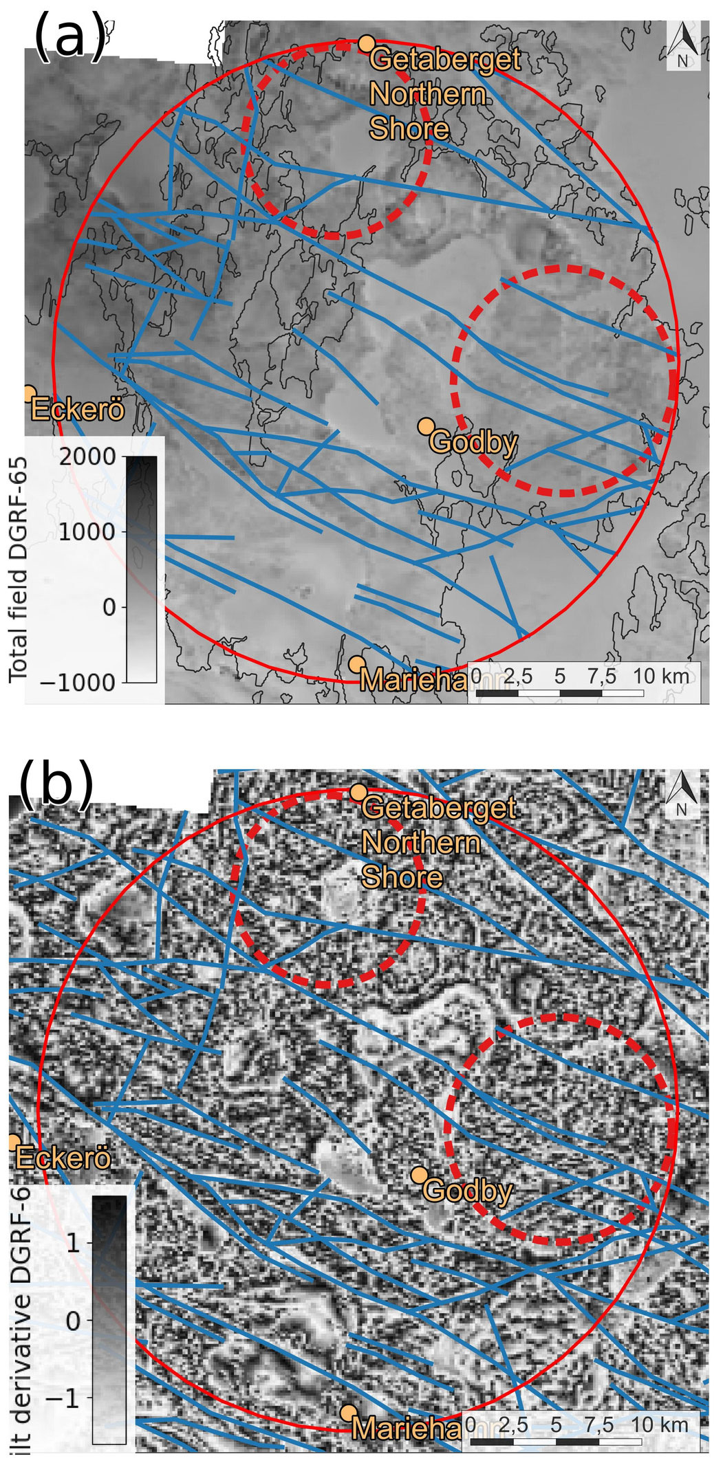
Figure A1 Magnetic lineaments that were interpreted using all three magnetic maps (sharp-filtered DGRF-65, total field DGRF-65 and tilt derivative DGRF-65) overlay both of the panels. (a) Total field DGRF-65 greyscale magnetic map used in magnetic lineament interpretation. (b)  Tilt derivative DGRF-65 greyscale magnetic map used in magnetic lineament interpretation.

Appendix B: Lognormal and exponential fits to full-length data

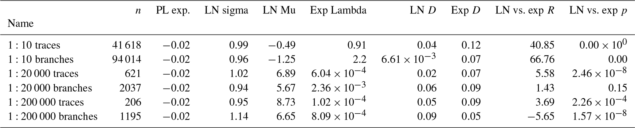
Full-length distributions of traces and branches for all scales are presented in Fig. B1, and the associated statistical characteristics are presented in Table B1. The lognormal fit is more probable than the exponential fit for all traces and branches, with the exception of 1:200 000-scale branch lengths, where the exponential fit is more probable with high statistical significance. The p values for the comparisons between lognormal and exponential fits are statistically significant (<0.1), with the exception of 1:20 000-scale branch lengths with a value of 0.15.

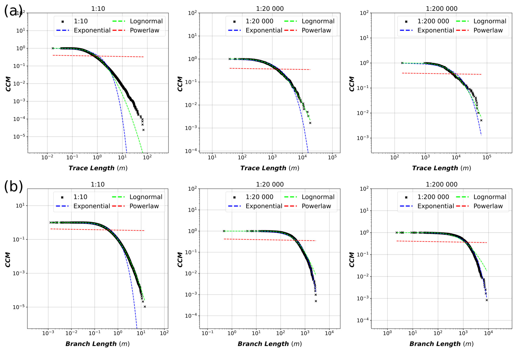
Figure B1 (a) Length distributions of traces of each scale on plots with complementary cumulative number (CCM) on the y axis and trace length on the x axis. The distributions are fitted with power-law, lognormal and exponential fits. (b) Length distributions of branches with the same setup as subfigure (a), except for the x axis, which has branch lengths rather than trace lengths.

Table B1 Parameters of power-law, lognormal and exponential length distribution fits for traces and branches for all scales without cut-offs. PL – power law. LN – lognormal. Exp – exponential. D – Kolmogorov–Smirnov distance. The R value is the log-likelihood ratio, where a positive value indicates that the lognormal fit is more likely and a negative value indicates that the exponential fit is more likely. The p value represents the significance of the likelihood where low values (<0.1) correspond to high statistical significance. Since the power law fails to model the lengths without cut-offs (Fig. B1), it is not compared statistically to the lognormal and exponential distributions.