the Creative Commons Attribution 4.0 License.
the Creative Commons Attribution 4.0 License.
 | 17 Jan 2024
Modeling liquid transport in the Earth's mantle as two-phase flow: effect of an enforced positive porosity on liquid flow and mass conservation
Changyeol Lee
Nestor G. Cerpa
Dongwoo Han
Ikuko Wada
Fluid and melt transport in the solid mantle can be modeled as a two-phase flow in which the liquid flow is resisted by the compaction of the viscously deforming solid mantle. Given the wide impact of liquid transport on the geodynamical and geochemical evolution of the Earth, the so-called “compaction equations” are increasingly being incorporated into geodynamical modeling studies. When implementing these equations, it is common to use a regularization technique to handle the porosity singularity in the dry mantle. Moreover, it is also common to enforce a positive porosity (liquid fraction) to avoid unphysical negative values of porosity. However, the effects of this “capped” porosity on the liquid flow and mass conservation have not been quantitatively evaluated. Here, we investigate these effects using a series of 1- and 2-dimensional numerical models implemented using the commercial finite-element package COMSOL Multiphysics®. The results of benchmarking experiments against a semi-analytical solution for 1- and 2-D solitary waves illustrate the successful implementation of the compaction equations. We show that the solutions are accurate when the element size is smaller than half of the compaction length. Furthermore, in time-evolving experiments where the solid is stationary (immobile), we show that the mass balance errors are similarly low for both the capped and uncapped (i.e., allowing negative porosity) experiments. When Couette flow, convective flow, or subduction corner flow of the solid mantle is assumed, the capped porosity leads to overestimations of the mass of liquid in the model domain and the mass flux of liquid across the model boundaries, resulting in intrinsic errors in mass conservation even if a high mesh resolution is used. Despite the errors in mass balance, however, the distributions of the positive porosity and peaks (largest positive liquid fractions) in both the uncapped and capped experiments are similar. Hence, the capping of porosity in the compaction equations can be reasonably used to assess the main pathways and first-order distribution of fluids and melts in the mantle.
- Article
(4579 KB) - Full-text XML
- BibTeX
- EndNote


The fluid and melt within the Earth's mantle, as well as their transport from depth to surface, play a key role in the geodynamical and geochemical evolution of our planet. At depth, the presence of small fluid and melt fractions (up to 1 %–10 %) affects the bulk physical properties of mantle rocks (Mei et al., 2002; Zimmerman and Kohlstedt, 2004; Dohmen and Schmeling, 2021). This effect partly influences the vigor of mantle convection (e.g., Ogawa and Nakamura, 1998) and potentially assists the localization of deformations (Holtzman et al., 2003; Zimmerman and Kohlstedt, 2004; Katz et al., 2006) and may thus be a key ingredient for the functioning of plate tectonics. At the depths at which they are generated and through their journey to the surface, fluid and melt extract incompatible and fluid-mobile elements from the mantle rocks, thereby controlling planetary differentiation and contributing to the growth of the continental crust (Gerya and Meilick, 2011; Jagoutz and Kelemen, 2015). The ascent and eruption of magmas lead to the formation of volcanoes over and between tectonic plates, linking the evolution of the solid Earth to the evolution of the atmosphere (Lopez et al., 2023).
Because of the wide impact that fluid and melt have on the Earth system, it is crucial to constrain their migration pathways and spatial distribution. These can be inferred on the basis of geophysical imaging (e.g., magnetotellurics and seismic tomography). However, such methods lead to interpretations that are often non-unique given the dependence of the observables on multiple factors. Further, they are only present-day static images of a dynamic process. Forward modeling of liquid transport is a tool that can help to quantify the fluid and melt migration and their spatial distribution in the mantle and to study the coupled fluid/melt-mantle dynamics at a geodynamic scale (from 1 to 100s of kilometers).
One of the pioneering studies on liquid (aqueous fluid and melt) transport in the solid Earth was that of McKenzie (1984) (see also Scott and Stevenson, 1984; Fowler, 1985), who derived a two-phase flow theory based on continuum mechanics for a liquid in a viscously deforming porous solid matrix (mantle rocks). In this theory, a buoyant liquid phase percolates through the solid phase, where the liquid viscosity is many orders of magnitude lower than that of the permeable mantle matrix. The liquid flow follows Darcy's law but experiences resistance due to the compaction of the solid matrix. Using this theory, liquid flow was evaluated in various geodynamic settings, including mid-ocean ridges (Katz, 2008; Keller and Katz, 2016; Cerpa et al., 2018; Sim et al., 2020; Pusok et al., 2022), subduction zones (Dymkova and Gerya, 2013; Wilson et al., 2014; Cerpa et al., 2017, 2018; Rees Jones et al., 2018; Wang et al., 2019), continental rifts (Schmeling, 2010; Li et al., 2023), and an intraplate context (Keller et al., 2013; Dannberg and Heister, 2016).
The mantle away from the vicinity of the plate boundaries is generally thought to be relatively dry except in the specific regions where the presence of volatiles and melts has been suggested, e.g., in the shallow asthenospheric mantle (Chantel et al., 2016; Cerpa et al., 2019; Debayle et al., 2020) and near the 410 and 660 km discontinuities (Bercovici and Karato, 2003). However, in the application of the two-phase flow equations to the mantle, the near-zero porosity limit leads to a singularity, and it is therefore difficult to handle numerically (Arbogast et al., 2017; Dannberg et al., 2019). Thus, the equations are commonly regularized by imposing a small porosity across the entire model domain (e.g., Wilson et al., 2014; Cerpa et al., 2017). Along with an assumption of small porosity, it is also necessary to “cap” the porosity field to avoid the development of negative porosity values, which naturally arises from the governing equations. However, despite the widespread use of a capped porosity in numerical models, its impacts on the liquid flow and mass conservation have not been quantitatively evaluated.
In the present study, we investigate the effect of regularization with the capped porosity on the liquid flow and mass conservation in the two-phase flow model for the Earth's mantle using the commercial finite-element package COMSOL Multiphysics® (COMSOL hereafter). COMSOL was used previously in the context of mantle convection and successfully benchmarked (e.g., Lee, 2013; Yu and Lee, 2018; Trim et al., 2021). For example, it was used to study the liquid transport in the mantle wedges of subduction zones when considering a simplified porous flow model that did not incorporate the effect of matrix compaction (e.g., Wada and Behn, 2015; Lee et al., 2021; Lee and Kim, 2021). It was also used to investigate compaction-driven segregation of porosity in shear bands (Butler, 2017). Here, we implement the governing equations that account for the compaction of the mantle matrix in COMSOL and validate the implementation by benchmarking the model solution against a semi-analytical solution for 1- and 2-dimensional (1- and 2-D) solitary waves. We then evaluate the effects of a capped porosity on liquid flow and mass conservation by comparing the mass balance between the capped and uncapped experiments using four different flow fields for the solid matrix: stagnant, Couette flow, convective flow, and subduction corner flow. One of the advantages of COMSOL is that it has the potential to perform coupling between different physics. Thus, the results of the present study can provide the basis for future applications of COMSOL for coupling the two-phase flow equations with other solid Earth processes, such as chemical reactions and heat transfer by liquids.
We follow the reformulation of the physics of two-phase flow in the mantle in which only the solid-state mantle flow (solid flow) influences the porous flow (i.e., one-way coupling) under the small-porosity approximation (e.g., Spiegelman, 1993; Katz et al., 2007; Katz, 2022). Such a formulation has been described in detail for previous studies which provided the derivation of the non-dimensionalized governing equations for the solid and liquid flow (Wilson et al., 2014; Cerpa et al., 2017). Below, we briefly describe the equations.
The governing equations for solid flow are the non-dimensionalized incompressible Stokes equations and the heat equation in a non-dimensionalized form (Wilson et al., 2014; Cerpa et al., 2017; Lee et al., 2021):
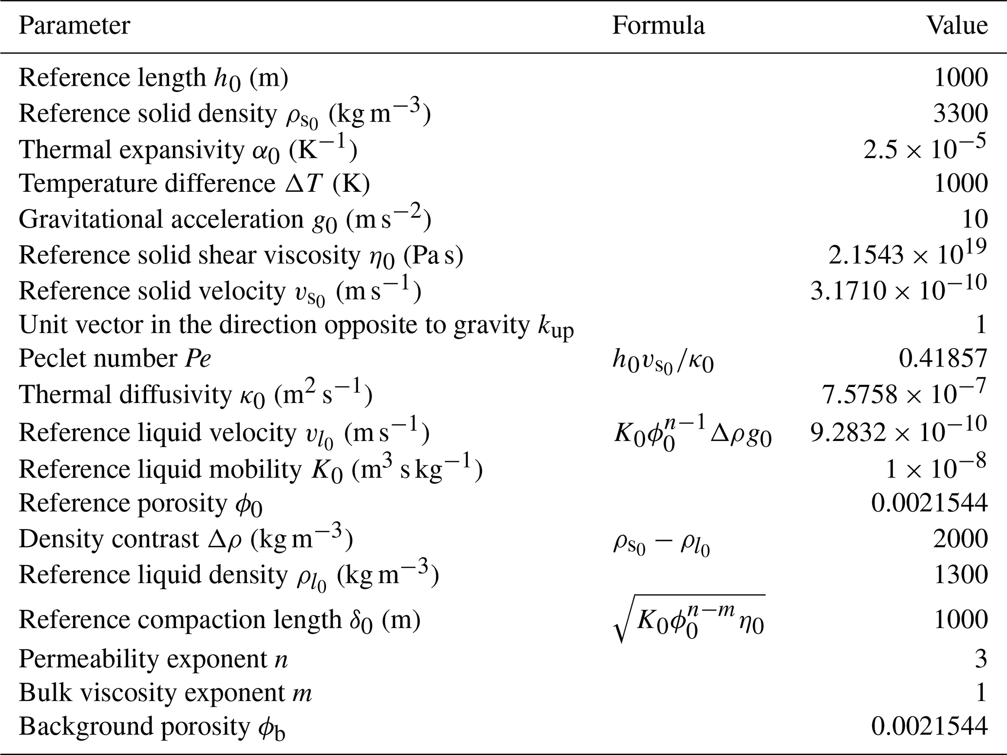
where vs is the solid velocity, η is the solid shear viscosity, is strain rate tensor, p is the dynamic pressure, h0 is the reference length, is the reference solid density, α0 is the thermal expansivity, ΔT is the temperature difference, g0 is the gravitational acceleration, η0 is the reference solid shear viscosity, is a reference solid velocity, T is the temperature, kup is the unit vector in the direction opposite to gravity, and Pe is the Peclet number (, where κ0 is the thermal diffusivity). In the heat equation, we neglect radiogenic heating and latent heat.
In what follows, we neglect the effect of the gradients of dynamic pressure term on the fluid flow since they are expected to be negligibly small compared to those of the compaction pressure in most of the regions of the convective mantle which we focus on (see discussion in Cerpa et al., 2017). Given this assumption, the non-dimensionalized governing equations for liquid flow are
where ϕ is the porosity, 𝒫 is the compaction pressure, ζ and K are the bulk viscosity and permeability, respectively, and Γ is the rate of mass transfer between the solid and liquid phases. The density contrast between the solid and liquid phases is denoted as (e.g., Wilson et al., 2014; Cerpa et al., 2017).
The reference compaction length δ0 is given by
where K0 is the reference liquid mobility (defined as the ratio of a reference permeability to a reference liquid viscosity), ϕ0 is the reference porosity, n is the permeability exponent, and m is the bulk viscosity exponent (Spiegelman, 1993). The reference liquid velocity is defined as
The non-dimensional bulk viscosity ζ, the permeability K, and the compaction length δ are, respectively,
Given the relationships shown in Eqs. (8) and (9), Eqs. (4) and (5) become singular if ϕ→0. In most geodynamic applications, the initial porosity field is close to zero away from the liquid pathways, so various approaches are employed to prevent a singularity (e.g., Wilson et al., 2014; Butler, 2017; Sim et al., 2020). Here, we use a regularized bulk viscosity and a regularized permeability defined as follows: and , where ϕϵ is a user-defined “small” porosity which can be chosen based on the choice of a minimum compaction length δϵ that presents the relationship (Wilson et al., 2014; Cerpa et al., 2017, 2018). Note that the regularized permeability is only applied to the term related to the gradients of the compaction pressure in Eq. (5). Finally, a negative porosity (ϕ<0) is physically unrealistic and thus a non-negative porosity field is commonly imposed as a constraint when solving the equations (e.g., Wilson et al., 2014; Cerpa et al., 2017, 2018). To evaluate the impact of such a treatment of the porosity field on liquid flow and mass conservation, we perform experiments with and without an enforced positive porosity (i.e., imposing ϕ = max (0, ϕ)). Hereafter, these experiments are referred to as “capped” and “uncapped” experiments, respectively.
For the Stokes equations (Eqs. 1 and 2), we use the Creeping Flow (CF) module in COMSOL with quadratic and linear elements for the velocity and pressure, respectively. For the heat equation (Eq. 3), we use the Heat Transfer in Fluids (HT) module with quadratic and continuous Galerkin finite elements. The standard stabilization methods for the streamline and crosswind diffusions are used for both the CF and HT modules. To solve the time-dependent equations (Eqs. 1–3), we use the generalized-alpha method, adopting second-order accuracy of time integration with the direct, fully coupled PARDISO solver.
Equation (4) is solved using the Transport of Diluted Species (TDS) module with the stabilization method for the streamline diffusion. Equation (5) is solved using the TDS module for a benchmarking experiment against a semi-analytical solution for 1- and 2-D solitary waves (Sect. 3), and the generalized Coefficient Form of PDE (CFPDE) module is used for all the other experiments (Sect. 4) because the CFPDE module is more flexible with the boundary conditions that can be applied (e.g., the Weak Contribution option). We applied the CFPDE module to solve Eq. (5) to test its consistency with the TDS module, and the porosity differences were found to be smaller than 10−9 (models not shown). We use the quadratic and continuous Galerkin finite elements for the spatial discretization of Eqs. (4) and (5). To solve the equations, the generalized-alpha method with second-order accuracy of time integration and the direct segregated PARDISO solver are used. The Jacobian is updated every time step. The Lower Limit option in the segregated solver in COMSOL is used to cap the porosity (ϕ = max (0, ϕ)).
3.1 Model setup
Simpson and Spiegelman (2011) derived a semi-analytical solution for a solitary wave which travels in the direction opposite to gravity (upward) at a fixed speed (c) without changing its shape. The solitary wave is kept stationary under an enforced downward solid velocity of c. We first benchmark our implementation of the equations against the semi-analytical solution for 1- and 2-D solitary waves. This benchmark allows us to verify the successful implementation of the equations in the steady-state limit before conducting time-evolving model experiments for which no analytical solution exists.
The governing equations for the solitary waves are as shown in Eqs. (4) and (5) with Γ=0. As in Simpson and Spiegelman (2011), we use and in both equations. The latter is based on a domain height that is 64 times the compaction length and is large enough to resolve the solitary waves without significant boundary effects. A structured mesh consisting of square elements is used to discretize the model domain. A pseudo-1-D model domain has a non-dimensionalized height of 1 and a width of two square element sizes, and the 2-D model domain is a square with a non-dimensionalized length of 1 in both dimensions. To solve the compaction pressure accurately, three or more nodes per compaction length should be used (Dohmen and Schmeling, 2021). We use an element size that is a quarter of the compaction length (i.e., ) unless otherwise stated. This is equivalent to a non-dimensionalized length of , which provides 9 nodes per compaction length and 513 nodes over the domain height. Since the initial non-dimensionalized porosity field is sufficiently large throughout the model domain (≥1), we set ϕϵ to 0 (i.e., no regularization). We prescribe unit non-dimensionalized porosity (ϕ=1) and zero compaction pressure (𝒫=0) at the top boundary as well as zero porosity gradient () and zero gradient of the compaction pressure () at the other boundaries.
The semi-analytic solution for a solitary wave defined for a particular choice of the triplet (c, n, m), where c, n, and m represent the non-dimensionalized speed of the solitary wave, the permeability exponent, and the bulk viscosity exponent, respectively, is imposed as an initial porosity field (e.g., Fig. 1b). We calculate the initial solution using the Python codes provided in the cookbook (TerraFERMA Cookbook; https://doi.org/10.6084/m9.figshare.1466786.v4, last access: 12 January 2024) of the open-source finite-element code TerraFERMA (Wilson et al., 2017). For accuracy, the solution is calculated at 513 evenly distributed nodes over the domain height, and the peak porosity is placed at the center of the model domain. Thus, all the nodes of the 1-D model have the exact values of the solution. For the nodes of the 2-D model domain, the solution is calculated at the nodes along the horizontal and vertical lines that pass through the center of the model domain, and the initial values at the other nodes are approximated by using a cubic spline interpolation. The solutions described on the model domain show hump- and cone-like shapes for one and two dimensions, respectively. Note that the initial compaction pressure is zero across the entire domain. Finally, a constant non-dimensionalized time step is set using a Courant number of 0.5 for the solid velocity, which in this case is identical to the velocity of the solitary wave. We run the model until a non-dimensionalized time of 0.5. In what follows, until stated otherwise, we provide non-dimensional parameter values (porosity, compaction pressure, time, etc.).
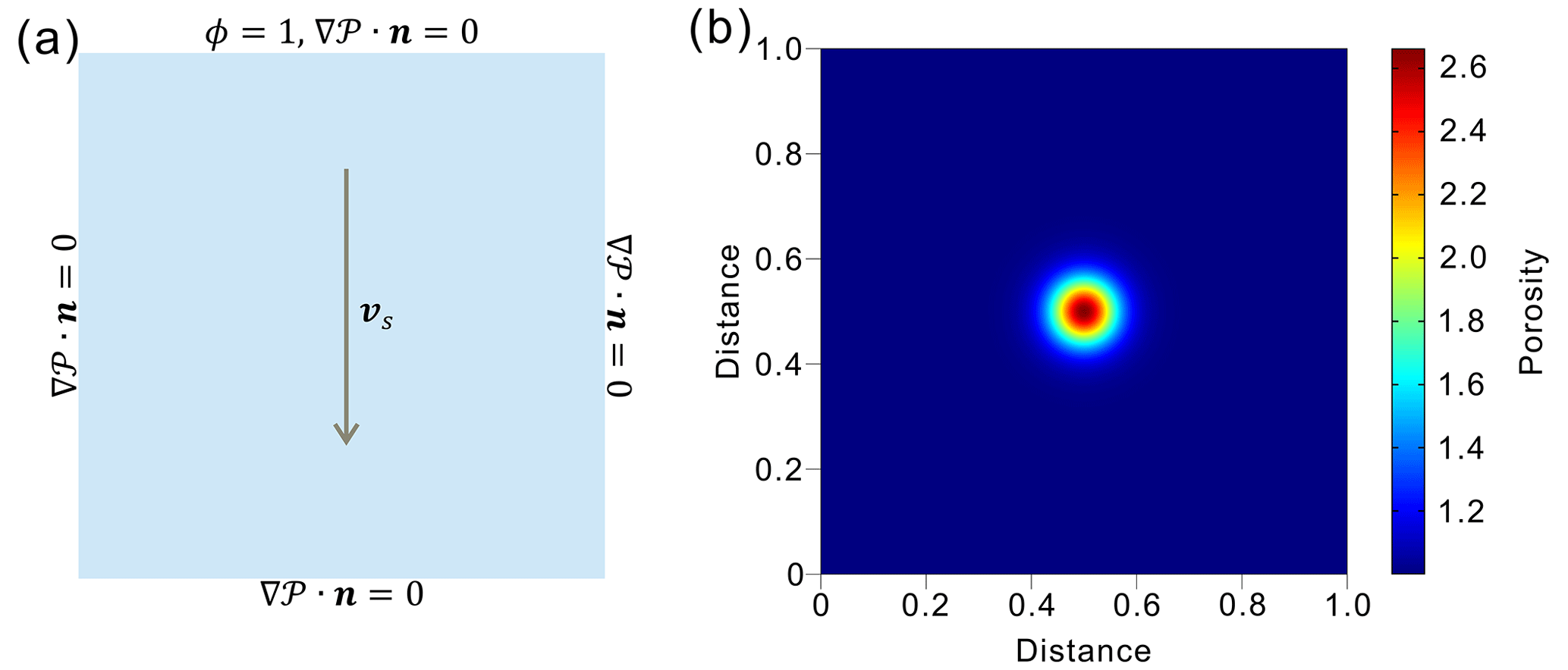
Figure 1(a) Model boundary conditions used for both the 1- and 2-D experiments. (b) Initial porosity from the 2-D experiment when the triplet (5, 3, 1) is chosen.
3.2 Benchmarking results
To quantify the growing error in the solitary wave with time, we calculate the phase shift and phase error of the wave relative to the semi-analytical solution along the vertical line that passes through the center of the model domain (e.g., Simpson and Spiegelman, 2011). The phase shift is estimated by tracking the location of the peak porosity value of the solitary wave relative to the central node (at a distance of 0.5) by fitting a second-order polynomial to the values at the central node and the nodes above and below it. The calculation of the phase error consists of two steps. First, the calculated porosity values at the nodes are interpolated using a piecewise cubic spline to obtain the waveform; then, the waveform is migrated back by the phase shift and the phase error is calculated over the nodes as follows:
where ∅calc,k is the value of the migrated waveform at the kth node, ∅anal,k is the corresponding value of the semi-analytical solution at the kth node, and l is the total number of nodes.
3.2.1 Effect of the choice of the triplet (c, n, m)
We benchmark the model solutions using three solitary wave solutions for different choices of the triplet (c, n, m): (4, 2, 1), (5, 3, 1), and (7, 3, 1). All the experiments show that the solitary wave undergoes a sudden downward migration after the first time step, yielding a negative phase shift on the order of (Fig. 2a) owing to the initial zero compaction pressure distribution. Then, it slowly migrates upwards with time. The experiments with the triplet (7, 3, 1) show the largest phase shifts: and for the 1- and 2-D experiments at a model time of 0.5, respectively; the phase shifts of the other experiments with triplets of (4, 2, 1) and (5, 3, 1) are smaller than 10−6 after a model time of 0.5. As observed in the phase shift, a sudden large phase error occurs after the first time step (on the order of 10−6 or smaller) and linearly increases with time (Fig. 2b). The linear increase in the phase error is likely due to numerical diffusion of the porosity field, which tends to smooth out the solitary wave.
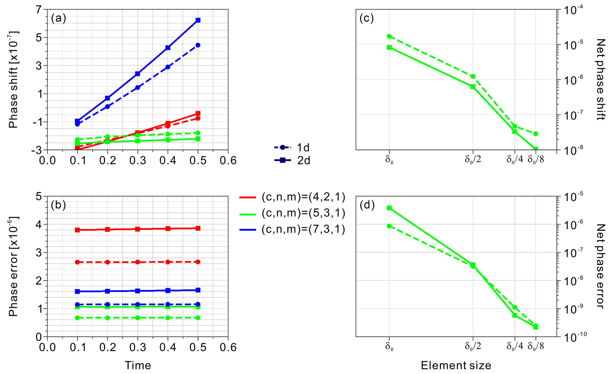
Figure 2(a, b) Time evolutions of the phase shifts and phase errors for the solitary waves calculated for three choices of the triplet (c, n, m) in the 1- and 2-D experiments. (c, d) Absolute net phase shifts and phase errors of the solitary waves calculated with the triplet (5, 3, 1) for element sizes of δ0, , , and in the 1- and 2-D experiments. These were calculated over a model time period of 0.4 (from a model time of 0.1 to 0.5).
3.2.2 Effect of the element size
We evaluate the effect of the element size on the solitary waves with the triplet (5, 3, 1). In addition to the reference experiment with an element size of mentioned above, we consider element sizes of δ0, , and (lengths of , , and , respectively). All other model parameters are the same as in the reference experiment.
The 1-D experiment using an element size of δ0 and both the 1- and 2-D experiments using an element size of show large phase shifts that grow with time (results not shown). This is because, in these experiments, a solitary wave originating from the top boundary passes the model domain toward the bottom boundary, which results in a substantial change in the shape of the existing solitary wave and forces the wave to migrate upward faster than in the other experiments. To minimize this “passing solitary wave” effect in these specific models, we used an initial condition field calculated at the evenly distributed 1025 nodes over the model height instead of 513 nodes. Using such a refined initial condition, the passing solitary wave does not occur in either 1- or 2-D experiments except in the 1-D experiment that uses the coarsest element size of δ0.
Overall, with the refined initial condition, the absolute net phase shift is relatively small () for all the element sizes that were tested except for δ0, which shows a much larger net phase shift () for the reason detailed above (Fig. 2c). As in the previous experiments, the phase error slowly grows with time, likely due to numerical diffusion of the porosity field (Fig. 2d). Moreover, an increase in mesh resolution leads to a decrease in the error. These experiments confirm that the higher the mesh resolution we use, the smaller the phase shift and phase error we observe.
Although the benchmark experiment is not designed for a specific spatiotemporal scale of geological interest, it is worth noting that the solution remains accurate up to a dimensional time of 0.05 Myr (the dimensional time using the model parameters shown in Table 1). The time-evolving problems described below consider longer timescales relevant to geological applications.
Although the benchmarking models described above verify the successful implementation of the compaction equations, the effects of the capped porosity on the liquid flow and mass conservation should be quantitatively evaluated. In the evaluation, we start with the simplest case – where the solid does not flow (a stagnant solid) – and then apply three solid-flow patterns that are applicable to Earth's mantle: Couette flow, convective flow, and subduction corner flow. Although no analytical solution exists for the modeling schemes, the relatively simple flow patterns that are applied in the models allow reasonable quantification of the sensitivity of liquid flow and mass conservation to the use of a capped porosity.
To monitor the accuracy of our computations over time, we evaluate the mass balance of the liquid (e.g., Lee et al., 2021). Since we assume a constant liquid density, this is equivalent to evaluating the volume balance of the liquid. The latter evaluation involves two steps. First, we evaluate the accumulated volume of liquid (Φacc) over the model domain by removing the initial total volume of liquid from the calculated total volume of liquid at a given time t. Second, we evaluate the net volume flux of liquid (Φflux) through the model liquid boundaries over a given time t. Both evaluations are conducted by assuming a unit thickness of the model domain (i.e., normal to the model domain) (e.g., Lee et al., 2021) as follows:
where ![]() is the volume integral over the model domain, while ϕ(t) and ϕ(0) are the porosity at a certain time t and at the initial model time t=0, respectively.
is the volume integral over the model domain, while ϕ(t) and ϕ(0) are the porosity at a certain time t and at the initial model time t=0, respectively. ![]() is the surface integral over the model boundaries. Note that positive and negative values of Φflux in Eq. (13) indicate a net volume outflux and a net volume influx, respectively. We use the trapezoidal rule with a constant time step for the time integration of the net volume flux of liquid.
is the surface integral over the model boundaries. Note that positive and negative values of Φflux in Eq. (13) indicate a net volume outflux and a net volume influx, respectively. We use the trapezoidal rule with a constant time step for the time integration of the net volume flux of liquid.
Theoretically, assuming that the time-integration scheme is accurate, the sum Φacc+Φflux should be equal to zero. In practice, a numerical error is expected to occur owing to the classical finite-element method itself and numerical integration of the liquid volume. Hence, we evaluate this relative volume-balance error as
In the subduction corner flow experiment, a liquid source is introduced within the uppermost slab layer. Thus, taking the liquid source into account, the relative volume-balance error is evaluated as
where Φsource is the liquid volume created within the uppermost slab layer over the model time, which is also calculated using the trapezoidal rule with a constant time step.
4.1 Liquid flow through a stagnant porous solid
4.1.1 Model setup
Firstly, we consider a 2-D time-evolving problem with a prescribed porosity at the bottom boundary of a square domain (the height and width are 50, equivalent to 50 km in dimensional units) of a stagnant (immobile) porous solid (Fig. 3a). We solve Eqs. (4) and (5) with Γ=0 using the model parameters described in Table 1 and the parameters that are specified below.
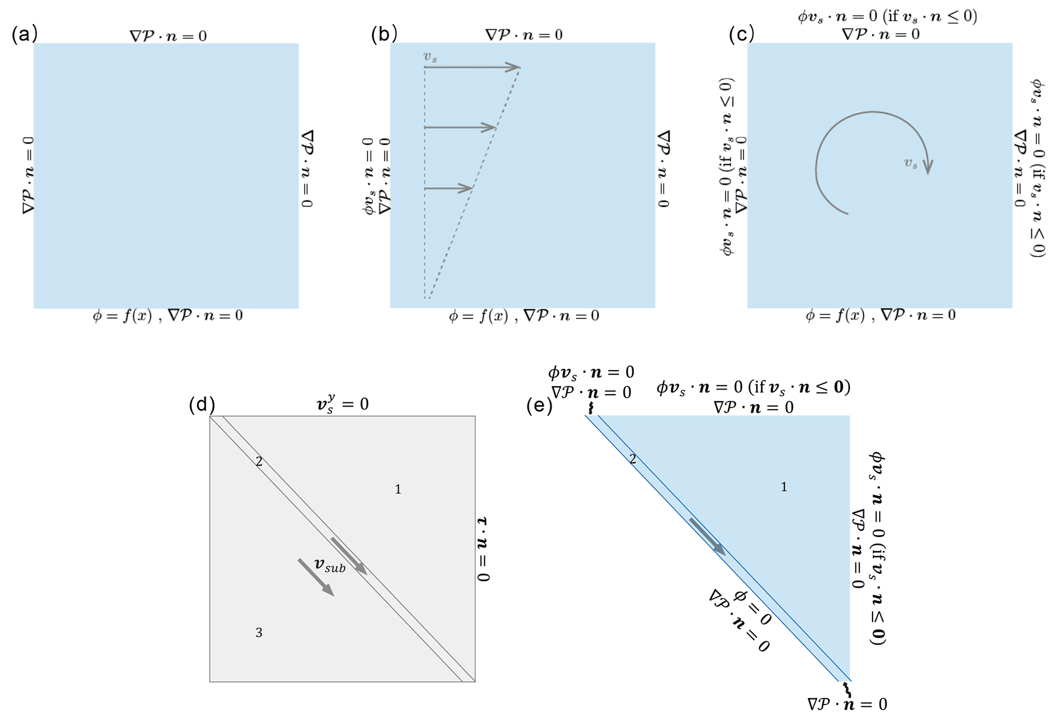
Figure 3Model boundary conditions used for the 2-D models of two-phase flow with four different solid flow patterns: (a) stagnant, (b) Couette flow, (c) convective flow, and (d, e) subduction corner flow.
The Dirichlet liquid boundary condition at the bottom boundary is specified using a Gaussian function:
where xc=25 (25 km) is the location of the maximum liquid and σ is the standard deviation, set equal to 1 (1 km). A zero compaction pressure gradient (i.e., a zero liquid flux condition) is prescribed at all the boundaries. The initial porosity field is set to zero over the entire domain.
A constant time step of 0.02 (2000 years) is used to satisfy the Courant criterion. The liquid flow is calculated for a model time of 300 (30 Myr). We use square elements of size (i.e., a length of ) to aid the accuracy of the solution (Dohmen and Schmeling, 2021).
4.1.2 Result
In both the capped and uncapped experiments, the solitary waves ascend vertically from the bottom boundary. With time, the waves tend to become vertically elongated, eventually merging into a channel with periodic highs and lows of porosity (Fig. 4a and b). In the uncapped experiment, negative porosity values down to occur near the ascending wave in the lower model domain. The negative porosity values tend to disappear as the wave passes through the upper model domain, and the entire porosity field is positive after a model time of ∼150. With time, the porosity fields in both experiments do not reach a steady state but instead exhibit a periodic behavior, resulting in a periodic integrated volume flux at the top wall boundary (Φflux, top) (Fig. 4c). Overall, the evolution of solitary waves is similar in both experiments.
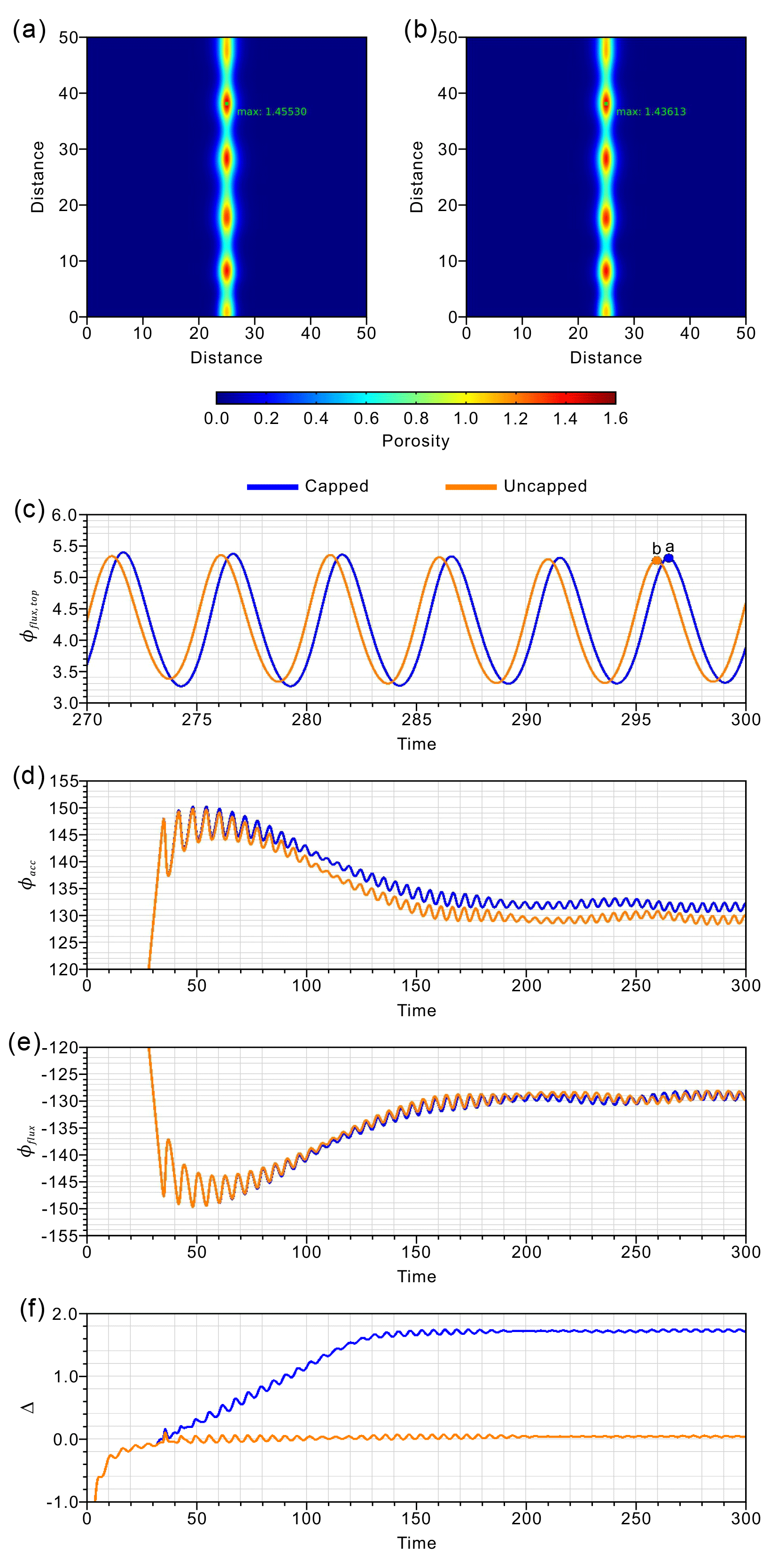
Figure 4(a, b) Snapshots of the porosity fields from the capped and uncapped experiments at model times of 296.50 and 295.96, respectively. The maximum porosities are depicted. (c) Evolution of the integrated volume flux through the top boundary (Φflux, top) in both experiments from a model time of 270 to a model time of 300. (d) The net accumulated volume of liquid (Φacc) over the model domain in both experiments from a model time of 0 to 300. (e) The net volume flux of liquid (Φflux) through the model liquid boundaries in both experiments from a model time of 0 to 300. (f) The relative volume-balance error (Δ) in both experiments from a model time of 0 to 300.
In the capped experiment, the accumulated volume of liquid (Φacc) first increases until a model time of 50 and then decreases to a stable value at a model time of ∼150 (Fig. 4d). The accumulated volume of liquid in the uncapped experiment follows a similar trend but is lower than that in the capped experiment after a model time of 50. The small difference in the stable value of Φacc between the experiments is solely due to the capping, which leads to a small overestimation of the integrated porosity over the model domain at each time step. The capped and uncapped experiments show a similar evolution of the net volume flux of liquid (Φflux) through the model boundaries (Fig. 4e). The negative sign of net volume flux indicates that the amount of liquid which enters through the bottom model boundary is larger than the amount which leaves the top boundary. The net volume flux also stabilizes after a model time of ∼150, indicating that the integrated volume influx of liquid is balanced by the integrated volume outflux of liquid through the model boundaries.
The evolution of the relative volume-balance error (Fig. 4f) illustrates the influence of the enforced positive porosity in the capped experiment. The enforcement results in an overestimation of the net accumulated volume of liquid until a model time of ∼150, yielding an increase in volume relative to that in the uncapped experiment (Fig. 4d). The negative porosity that is allowed in the uncapped experiment leads to a smaller accumulated volume of liquid and a more accurate volume balance. By a model time of 300, the relative errors in the capped and uncapped experiments are 1.71 % and of the order of 10−2 %, respectively.
4.2 Liquid flow through a Couette flow of a porous solid
4.2.1 Model setup
Here, we consider the evolution of a liquid flow through a Couette flow of a porous solid from left to right (maximum solid velocity: 3, equal to 3 cm yr−1) using the same model domain, boundary conditions, and methods shown in Sect. 4.1.1 (Fig. 3b). No porosity is brought in by the Couette flow across the left boundary.
4.2.2 Result
Due to the Couette flow, the solitary waves originating from the bottom boundary are diverted rightwards in both the capped and uncapped experiments (Fig. 5a and b). With time, the solitary waves tend to form channels displaying periodic highs and lows of porosity in both experiments, leading to very similar peak volume outfluxes of liquid at the right boundary (Fig. 5c). However, the uncapped experiment additionally develops two negative-porosity channels under the positive-porosity channel, yielding negative-volume outfluxes of liquid at the right boundary (at y coordinates ranging from 29.62 to 45.52 and from 47.46 to 48.85).
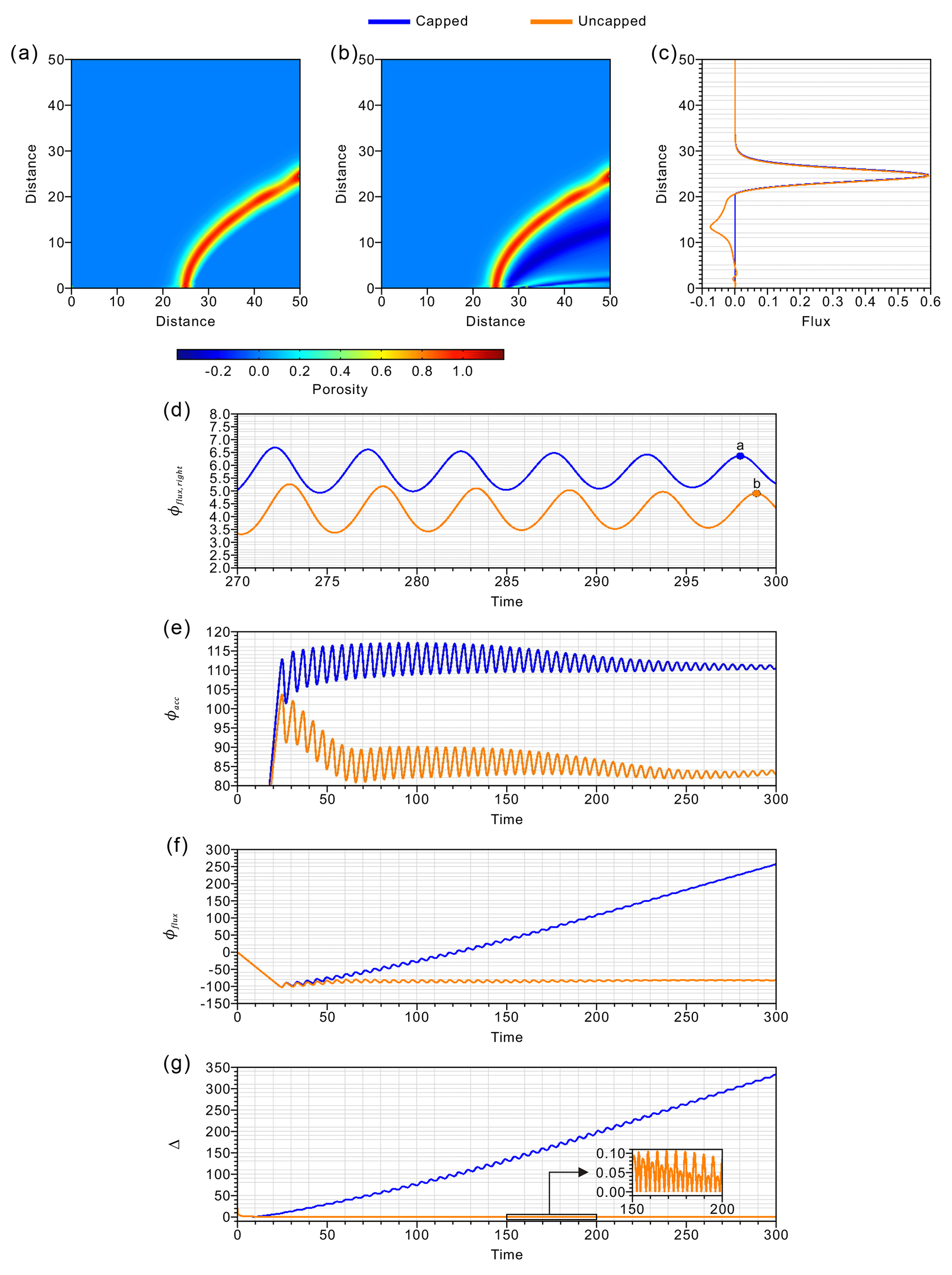
Figure 5(a, b) Snapshots of the non-dimensional porosity fields from the capped and uncapped experiments at model times of 298.02 and 298.92, respectively. The maximum and minimum porosities are depicted. (c) Volume fluxes over the right boundary from both experiments at the model times shown in panels (a) and (b). (d) Evolution of the integrated volume flux through the right boundary (Φflux, right) from both experiments at model times from 270 to 300. (e) The net accumulated volume of liquid (Φacc) over the model domain from both experiments. (f) The net volume flux of liquid (Φflux) through the model liquid boundaries from both experiments. (g) The relative volume-balance error (Δ) in both experiments from a model time of 0 to 300.
The time evolutions of the integrated volume outfluxes of liquid at the right boundary (Φflux, right) show that the fluxes slowly and asymptotically converge (Fig. 5d). Additional experiments were performed for a longer model time of 1000, and those reached a steady state (not shown). The capped experiment shows a larger Φacc than the uncapped experiment from the early stages to the end of the modeling period (Fig. 5e). In particular, the asymptotic value of Φacc in the capped experiment remains approximately 30 % higher than that in the uncapped experiment. The net volume fluxes of liquid in the two experiments show a pronounced divergence in behavior after a modeling time of ∼25 (Fig. 5f). While Φflux in the capped experiment increases with time from negative values (indicating an influx) in the early stages to positive values (indicating an outflux) in the later stages, Φflux stabilizes to an apparent steady state in the uncapped experiment. This indicates that the integrated volume outflux exceeds the integrated volume influx through the model boundaries in the capped experiment. On the contrary, the stable value of Φflux in the uncapped experiment indicates that the integrated volume influx of liquid is balanced by the integrated volume outflux of liquid through the model boundaries. Both Φacc and Φflux are well balanced in the uncapped experiment, and the relative volume-balance error remains very small (0.09 % at a model time of 300). Similar to the behavior of Φflux, the relative volume-balance error in the capped experiment greatly and continuously increases with model time (reaching 332 % at a model time of 300) even after the model starts to reach a steady state, whereas the error in the uncapped experiment diminishes with time (Fig. 5g).
The enforced positive porosity in the capped experiment leads to a larger net accumulated volume of liquid compared to that in the uncapped experiment, in which the accumulated volume is counterbalanced by negative porosity. Thus, Φacc is overestimated in the capped experiment relative to the uncapped experiment, and the higher accumulated porosity leads to an overestimation of the integrated volume outflux through the right boundary, as seen in the distribution of volume flux (Fig. 5c) and the integrated value over time (Fig. 5d). The increase in the outflux is not sufficient to completely offset the increase in the accumulated porosity. As a consequence, the accumulated porosity, the net volume (out)flux of liquid through the model boundaries, and the relative volume-balance error continuously increase (Fig. 5e and f).
4.3 Liquid flow through a convective porous solid
4.3.1 Model setup
Here, we consider the evolution of the liquid flow through a convective porous solid using the same model domain, boundary conditions, and methods shown in Sect. 4.1.1 (Fig. 3c). We apply free slip to all four boundaries to solve the solid flow. To solve the heat equation, the top and bottom temperatures are fixed at 0 and 1 (0 and 1000 ∘C), respectively, and the left and right walls are prescribed as having a zero heat-flux boundary condition. The quasi-steady state convective flow is first calculated by solving Eqs. (1)–(3) for a model time of 500 (50 Myr). Then, the liquid flow is calculated for a model time of 300 (30 Myr). No porosity influx by solid advection is allowed across any of the four boundaries, whereas porosity outflux is allowed (i.e., there are free-outflux and zero-influx boundary conditions).
4.3.2 Results
Due to the clockwise solid convection, the solitary waves ascending from the bottom boundary are diverted leftwards and rightwards in the lower and upper model domains, respectively, in both the capped and uncapped experiments (Fig. 6a and b). Most of the ascending liquid leaves the domain through the top boundary, but a fraction of it continues to be entrained in the convective solid and remains within the domain. The entrained liquid then merges with newly ascending liquid from the bottom boundary. With time, the waves tend to form a quasi-steady-state channel in the capped experiment, which leads to a quasi-steady-state integrated volume outflux of liquid (which slowly increases) through the top boundary (Φflux, top) (Fig. 6c). On the contrary, the porosity field in the uncapped experiment does not converge to a steady state by the end of the modeling period. This also leads to an unsteady integrated volume outflux of liquid through the top boundary. Negative porosity values occur near the liquid pathway by the end of the modeling period, decreasing the integrated volume outflux of liquid at the top boundary.
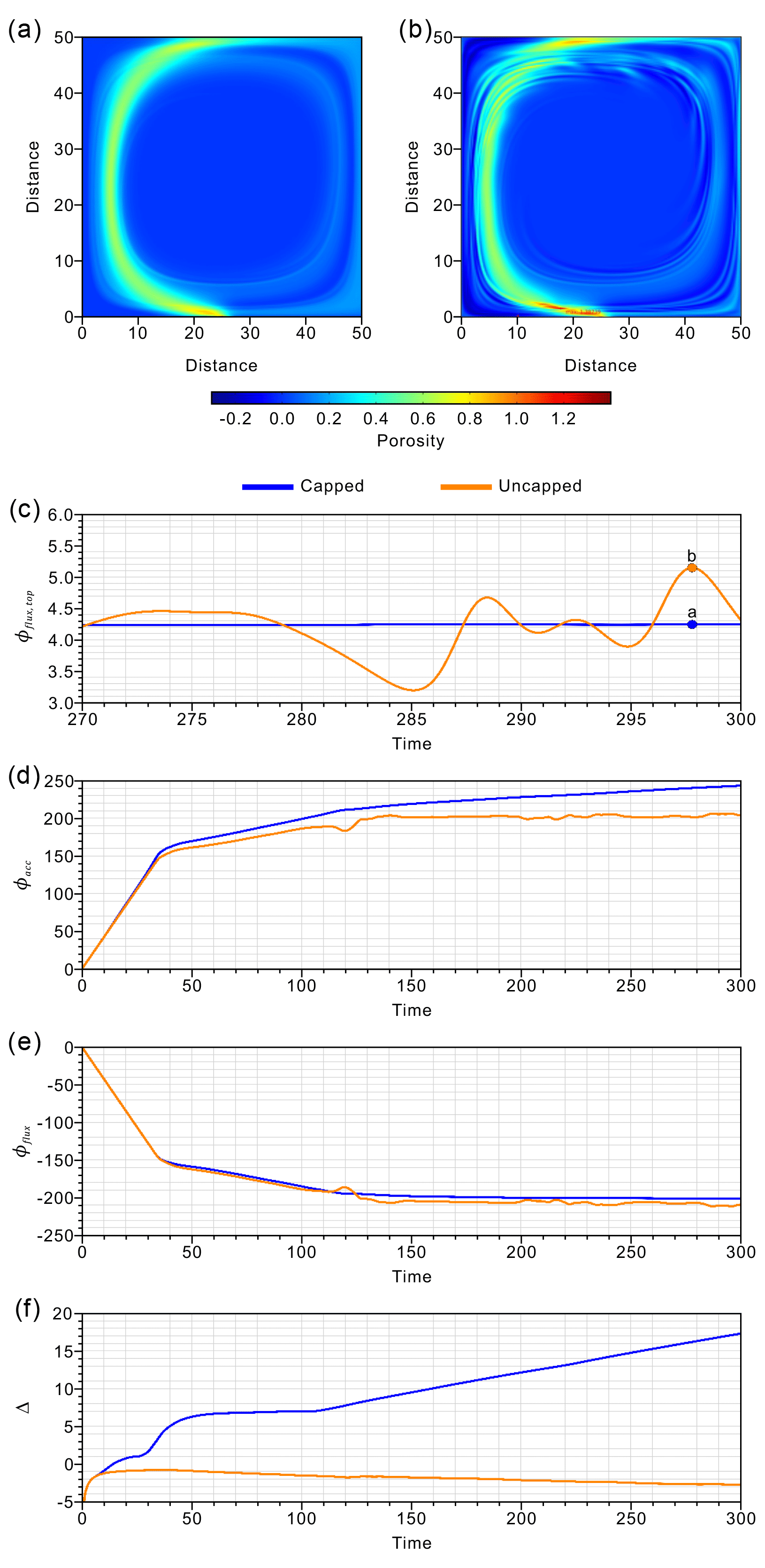
Figure 6(a, b) Snapshots of the non-dimensional porosity fields from the capped and uncapped experiments at a model time of 297.80. The maximum and minimum porosities are depicted. (c) Evolution of the integrated volume flux through the top boundary (Φflux, top) in both experiments from a model time of 270 to 300. (d) The accumulated volume of liquid (Φacc) over the model domain from both experiments. (e) The net volume flux of liquid (Φflux) through the model liquid boundaries from both experiments. (f) The relative volume-balance error (Δ) in both experiments from a model time of 0 to 300.
In both the capped and uncapped experiments, the evolution of Φacc can be divided into three stages (Fig. 6d). First, there is a transient stage (0 to ∼40) corresponding to the time taken for the first solitary wave to ascend through the model domain and reach the top boundary. A second transient stage (∼40 to ∼120) corresponds to the time taken for a fraction of the liquid of the first solitary wave to be advected downwards by the convective cell and merge with solitary waves that have entered the domain and ascended from the bottom boundary. The second stage ends when these merged solitary waves reach the top domain. A third stage (∼120 to the end) corresponds to the period in which the entrained liquid continues to merge with the solitary waves that ascend from the bottom boundary and the rotating porosity channel reaches a semi-steady state. The capped experiment shows an increasing Φacc during all of these stages, even in the third stage, whereas the uncapped experiment shows a stable value during the third stage. On the contrary, the net volume fluxes of liquid (Φflux) are equally stable (they very slowly decrease) in both experiments after a model time of ∼150 in the third stage (Fig. 6e). The relative volume-balance error (Δ) in the capped experiment displays a net increase with time and reaches 17.3 % at a model time of 300. However, in the uncapped experiment, it slowly decreases with time and reaches −2.8 % at the same time (Fig. 6f).
As in Sects. 4.1 and 4.2, the enforced positive porosity in the capped experiment results in an overestimation of Φacc. The overestimation is relatively small until a model time of ∼30 but becomes significantly larger when the first porosity wave reaches the top boundary at a model time between ∼30 and ∼40. Between model times of ∼30 and ∼40, we also observe a slightly higher Φflux in the capped experiment, which indicates that the outflux is slightly larger than that in the uncapped experiment owing to the enforced positive porosity. The relative volume-balance error also undergoes a fast increase between model times of ∼30 and ∼40 in the capped experiment, which is not observed in the uncapped experiment. During the second stage, the impact of the enforced positive porosity on Φacc is relatively small, as illustrated by the similar evolution of Φacc in the two experiments before a model time of ∼120. Thus, both experiments show stable relative volume-balance errors, though a slight decrease in the relative volume-balance error with time is observed in the uncapped experiment. During the third stage, however, large divergences between the experiments are seen in Φacc and the relative volume-balance error. The enforced positive porosity mostly impacts Φacc, which undergoes a substantial increase with time in the capped experiment. This is because the overestimated Φacc progressively impacts newly ascending liquid volumes. On the contrary, although Φflux is always slightly larger in the capped experiment, the difference in Φflux between the experiments remains stable throughout the third stage. This shows that the continuous increase in relative volume-balance error recorded in the capped experiment is solely due to the overestimation of Φacc. As observed for the previous models (Sects. 4.1 and 4.2), the volume balance is better maintained in the uncapped experiment.
4.4 Liquid flow through a subduction corner flow
4.4.1 Model setup
Lastly, we consider the evolution of the liquid flow through a subduction corner flow in which the solid-state flow in the corner wedge is kinematically driven by the subducting slab. The height and width of the model are 50 and 52.8 (equal to 50 and 52.8 km), respectively (Fig. 3d). The subducting slab has a dip of 45∘ and a subduction rate of 5 (5 cm yr−1).
To solve the solid flow, free-slip and open-boundary conditions are prescribed for the top and right boundaries of the mantle wedge, respectively (Fig. 3d). To reach steady-state corner flow in the mantle wedge, Eqs. (1) and (2) without the buoyancy term in Eq. (2) are solved for a modeling period of 500 (50 Myr) (e.g., Yu and Lee, 2018).
To solve the liquid flow, free-outflux and zero-influx boundary conditions are prescribed for all the boundaries except for the base of the uppermost slab layer, which is prescribed as having zero porosity (Fig. 3e). A zero gradient of compaction pressure is prescribed for all the boundaries. A Gaussian source term (the same function as in Eq. 16) for Γ in Eqs. (4) and (5) is applied within the uppermost slab layer over a thickness of 2 (2 km). The source term is a simplified proxy for a dehydration reaction that would produce some liquid within the uppermost slab layer. To discretize the slab and wedge geometry, we use an unstructured mesh consisting of triangular elements that are slightly smaller than a quarter of the compaction length. The liquid flow is calculated by solving Eqs. (4) and (5) for a model time of 300 (30 Myr) with a constant time step of 0.004 (400 years).
4.4.2 Results
The general trends for the liquid flow in the wedge are similar in both the capped and uncapped experiments, both of which tend toward stable dynamics after a model time of 50. Due to the downdip solid flow, the solitary waves originating from the top layer tend to be diverted slightly rightwards as they ascend through the bottom half of the wedge. In the top half of the wedge, the inward (leftward) corner flow causes leftward advection of the ascending waves before they reach the top boundary (Fig. 7a and b). Although most of the liquid passes upward through the wedge, a fraction of it is entrained by the corner flow and leaves the model domain across the right boundary.
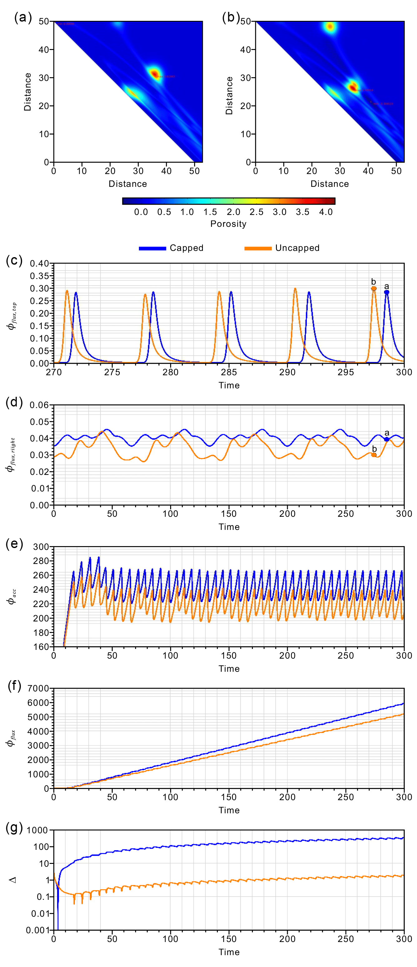
Figure 7(a, b) Snapshots of the non-dimensional porosity fields from the capped and uncapped experiments at model times of 298.52 and 297.42, respectively. The maximum and minimum porosities are depicted. (c, d) Evolution of the integrated volume flux through the top and right boundaries (Φflux, top and Φflux, right) in both experiments from a model time of 270 to 300. (e) The accumulated volume of liquid (Φacc) over the model domain from both experiments. (f) The net volume flux of liquid (Φflux) through the model liquid boundaries from both experiments. (g) The absolute volume-balance relative error (Δ) in both experiments from a model time of 0 to 300.
Both the capped and uncapped experiments yield periodic high and low volume fluxes at the top and right boundaries (Φflux, top and Φflux, right). These fluxes correspond to solitary waves reaching the top boundary after their ascent from the top of the subducting slab and to the downdip advection of a fraction of them, respectively (Fig. 7c and d). The amplitudes and periods of the volume fluxes at the top boundary remain very similar in both experiments. At the right boundary, the periods of the volume fluxes are also very similar, but the amplitude at the right boundary is larger in the capped experiment.
Compared to that in the capped experiment, the uncapped experiment shows a lower Φacc due to the negative porosity field in the model domain. Similarly, Φflux is lower, due to the lower outflux at the right boundary (Fig. 7e and f). As a result, the difference in Φflux between the experiments increases with time. The capped experiment yields a relative volume-balance error of 337.17 % at a model time of 300, whereas it is only −1.85 % in the uncapped experiment. (Fig. 7g). Thus, a better balance between Φacc and Φflux is maintained when negative porosity is allowed in the uncapped experiment.
4.5 Effect of element size on the relative error in time-dependent problems
To check the sensitivity of our results to the choice of element size, we run additional experiments with square element sizes of , , and (lengths of , , and , respectively), which provide 5, 17, and 33 nodes per compaction length, respectively, for the stagnant solid, Couette flow, and convective flow experiments. For the subduction corner flow experiment, triangular elements with sizes that are slightly smaller than , , and are additionally considered. We run all the experiments up to a model time of 300.
All the stagnant porous solid experiments show similar porosity evolutions regardless of the element size chosen. It is important to note that the uncapped and capped experiments converge towards different minimum errors. A significant decrease in the relative volume-balance error is observed with increasing mesh resolution in the uncapped experiments; the error diminishes to % in the experiment using the finest mesh resolution (Fig. 8a). The error in the capped experiments slightly decreases with increasing mesh resolution (from ∼1.83 % to ∼1.69 % over the range of mesh resolutions), but a relatively large error remains regardless of the mesh resolution. This indicates that enforced positive porosity results in intrinsic errors due to overestimations of the porosity in the model domain and the outflux at the top boundary.
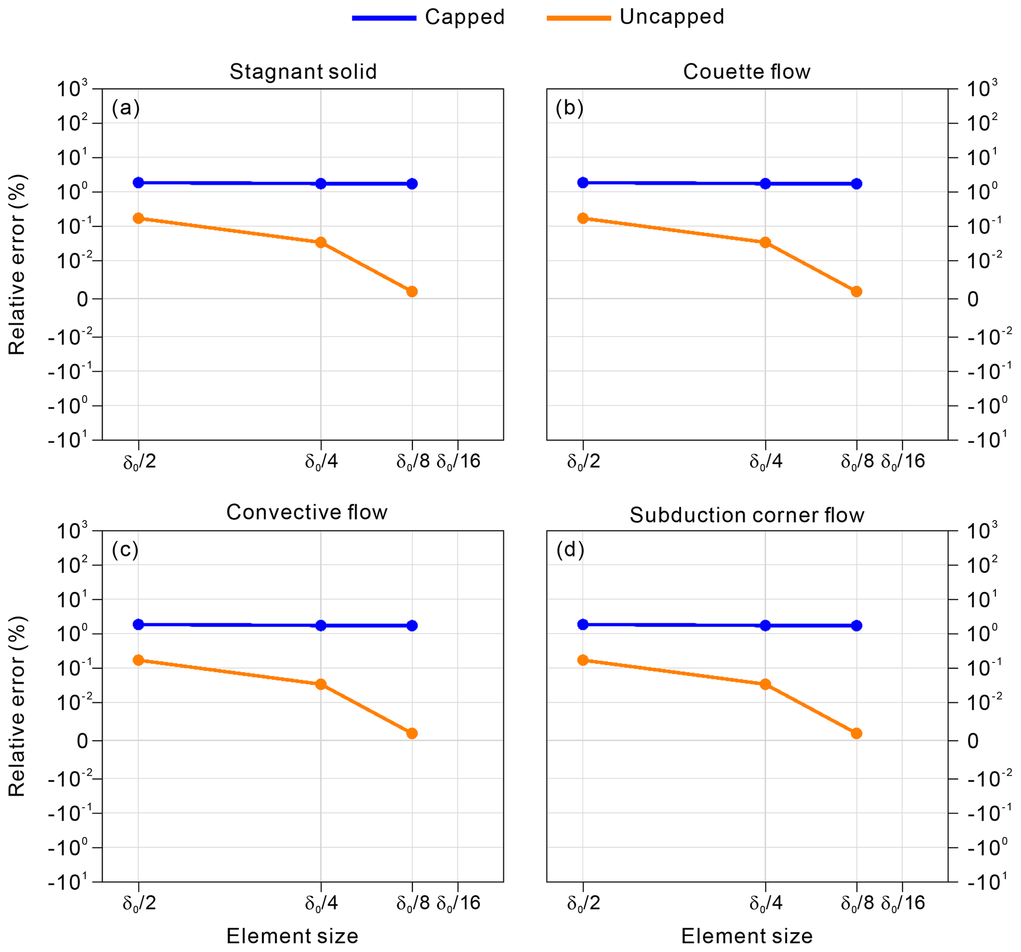
Figure 8Relative volume-balance error calculated from capped and uncapped experiments with various element sizes ranging between and : (a) stagnant solid, (b) Couette flow, (c) convective flow, and (d) subduction corner flow.
All the other experiments (those for Couette flow, convective flow, and subduction corner flow) show similar porosity evolutions regardless of the element size chosen. In all cases, the uncapped experiment always shows better liquid volume conservation (i.e., smaller absolute error values) with the increase in mesh resolution because the outflux at the boundaries is more accurately calculated at increased mesh resolution (Fig. 8b–d). The increase in mesh resolution in the capped experiments does not remove the intrinsic error that results from the overestimated porosity in the model domain and the subsequent overestimation of the outflux at the boundaries, though the outflux at the boundaries is more accurately calculated at increased mesh resolution.
In this study, we first conducted a series of benchmarking experiments against a semi-analytical solution for solitary waves (Simpson and Spiegelman, 2011). Although the specifics of the numerical approach used in the study (nonlinear solvers, finite element order, continuous Galerkin finite elements, etc.) differ from those used in previous studies (e.g., Simpson and Spiegelman, 2011; Wilson et al., 2017; Wang et al., 2019), we obtain a relatively accurate solution when the element size is or smaller (i.e., five or more nodes per compaction length). The impact of element size on the solution accuracy is consistent with previous studies (Dohmen and Schmeling, 2021), and, as expected, increasing the mesh resolution (decreasing the element size) significantly improves the solution accuracy, partly owing to a reduced numerical diffusion of porosity.
Next, we performed time-evolving experiments. Our capped experiments show that the best accuracy for mass conservation occurs in models where the background mantle is stationary (Figs. 4a and 8a) after those models have passed their early stages. In other experiments where the solid flows (Couette flow, convective flow, and subduction corner flow), the error in the mass balance is not negligible owing to the overestimation of porosity induced by the capped porosity and the subsequent overestimation of the mass flux across the model boundaries. Because the overestimation in the capped experiments is intrinsic, increasing the mesh resolution does not significantly reduce the relative volume-balance error (Fig. 8). Thus, the estimated volume of liquid in the model domain and the volume flux of liquid through the model boundaries (e.g., the amount of magma in the mantle and the migration of magma through the overlying lithosphere) should be carefully interpreted when the solid phase is deforming. We thus emphasize that, in future applications, caution should be taken when using the melt and flux estimations. However, the distributions of the positive porosity and peaks (the largest positive liquid fractions) in the model domain and boundaries, respectively, are quite similar in both the capped and uncapped experiments. Hence, it is reasonable to use a capped porosity in the compaction equations for assessing the main fluid pathways and the first-order distribution of fluids and melts in the mantle. Models of liquid transport in the mantle with a capped porosity field may be compared to geophysical imaging (e.g., magnetotellurics and seismic tomography) of the asthenosphere, which illuminates the first-order distribution of fluids and melts in, for example, the sub-arc mantle wedges of subduction zones (Mcgary et al., 2014; Cordell et al., 2019; Bie et al., 2022).
The models were run with the commercial finite-element package COMSOL Multiphysics® (https://www.COMSOL.com, COMSOL, 2023).
The data used to generate the figures are shared at https://doi.org/10.5281/zenodo.8179527 (Lee et al., 2023).
CL and NC conceived the study. CL and NC designed and ran the models, analyzed the results, and wrote the article. DH revised the Python code for the benchmarking experiments and produced the figures. IW wrote the article. All authors discussed the results and their consequences and contributed to the writing of the final article.
The contact author has declared that none of the authors has any competing interests.
Publisher’s note: Copernicus Publications remains neutral with regard to jurisdictional claims made in the text, published maps, institutional affiliations, or any other geographical representation in this paper. While Copernicus Publications makes every effort to include appropriate place names, the final responsibility lies with the authors.
We thank the editor Juliane Dannberg, the reviewer Samuel Butler, an anonymous reviewer, and Chenyu Tian for their constructive comments which have improved our manuscript.
This research has been supported by the National Research Foundation of Korea (grant no. 2022R1A2C1004592 for CL and DH) and the National Science Foundation (grants no. EAR-2246804 for IW).
This paper was edited by Juliane Dannberg and reviewed by Samuel Butler and one anonymous referee.
Arbogast, T., Hesse, M. A., and Taicher, A. L.: Mixed Methods for Two-Phase Darcy–Stokes Mixtures of Partially Melted Materials with Regions of Zero Porosity, SIAM J. Sci. Comput., 39, B375–B402, https://doi.org/10.1137/16m1091095, 2017.
Bercovici, D. and Karato, S.-i.: Whole-mantle convection and the transition-zone water filter, Nature, 425, 39–44, https://doi.org/10.1038/nature01918, 2003.
Bie, L., Hicks, S., Rietbrock, A., Goes, S., Collier, J., Rychert, C., Harmon, N., and Maunder, B.: Imaging slab-transported fluids and their deep dehydration from seismic velocity tomography in the Lesser Antilles subduction zone, Earth Planet. Sci. Lett., 586, 117535, https://doi.org/10.1016/j.epsl.2022.117535, 2022.
Butler, S. L.: Shear-induced porosity bands in a compacting porous medium with damage rheology, Phys. Earth Planet. In., 264, 7–17, https://doi.org/10.1016/j.pepi.2016.12.006, 2017.
Cerpa, N. G., Rees Jones, D. W., and Katz, R. F.: Consequences of glacial cycles for magmatism and carbon transport at mid-ocean ridges, Earth Planet. Sci. Lett., 528, 115845, https://doi.org/10.1016/j.epsl.2019.115845, 2019.
Cerpa, N. G., Wada, I., and Wilson, C. R.: Fluid migration in the mantle wedge: Influence of mineral grain size and mantle compaction, J. Geophys. Res.-Sol. Ea., 122, 6247–6268, https://doi.org/10.1002/2017jb014046, 2017.
Cerpa, N. G., Wada, I., and Wilson, C. R.: Effects of fluid influx, fluid viscosity, and fluid density on fluid migration in the mantle wedge and their implications for hydrous melting, Geosphere, 15, 1–23, https://doi.org/10.1130/ges01660.1, 2018.
Chantel, J., Manthilake, G., Andrault, D., Novella, D., Yu, T., and Wang, Y.: Experimental evidence supports mantle partial melting in the asthenosphere, Sci. Adv., 2, e1600246, https://doi.org/10.1126/sciadv.1600246, 2016.
COMSOL: Commercial finite-element package, COMSOL Multiphysics® [ver. 5.6], https://www.COMSOL.com, 2023.
Cordell, D., Unsworth, M. J., Diaz, D., Reyes-Wagner, V., Currie, C. A., and Hicks, S. P.: Fluid and Melt Pathways in the Central Chilean Subduction Zone Near the 2010 Maule Earthquake (35–36∘ S) as Inferred From Magnetotelluric Data, Geochem. Geophy. Geosy., 20, 1818–1835, https://doi.org/10.1029/2018GC008167, 2019.
Dannberg, J. and Heister, T.: Compressible magma/mantle dynamics: 3-D, adaptive simulations in ASPECT, Geophys. J. Int., 207, 1343–1366, https://doi.org/10.1093/gji/ggw329, 2016.
Dannberg, J., Gassmöller, R., Grove, R., and Heister, T.: A new formulation for coupled magma/mantle dynamics, Geophys. J. Int., 219, 94–107, https://doi.org/10.1093/gji/ggz190, 2019.
Debayle, E., Bodin, T., Durand, S., and Ricard, Y.: Seismic evidence for partial melt below tectonic plates, Nature, 586, 555–559, https://doi.org/10.1038/s41586-020-2809-4, 2020.
Dohmen, J. and Schmeling, H.: Magma ascent mechanisms in the transition regime from solitary porosity waves to diapirism, Solid Earth, 12, 1549–1561, https://doi.org/10.5194/se-12-1549-2021, 2021.
Dymkova, D. and Gerya, T.: Porous fluid flow enables oceanic subduction initiation on Earth, Geophys. Res. Lett., 40, 5671–5676, https://doi.org/10.1002/2013gl057798, 2013.
Fowler, A. C.: A mathematical model of magma transport in the asthenosphere, Geophys. Astro. Fluid, 33, 63–96, https://doi.org/10.1080/03091928508245423, 1985.
Gerya, T. V. and Meilick, F. I.: Geodynamic regimes of subduction under an active margin: effects of rheological weakening by fluids and melts, J. Metamorph. Geol., 29, 7–31, https://doi.org/10.1111/j.1525-1314.2010.00904.x, 2011.
Holtzman, B. K., Groebner, N. J., Zimmerman, M. E., Ginsberg, S. B., and Kohlstedt, D. L.: Stress-driven melt segregation in partially molten rocks, Geochem. Geophy. Geosy., 4, 8607, https://doi.org/10.1029/2001GC000258, 2003.
Jagoutz, O. and Kelemen, P. B.: Role of Arc Processes in the Formation of Continental Crust, Annu. Rev. Earth Pl. Sc., 43, 363–404, https://doi.org/10.1146/annurev-earth-040809-152345, 2015.
Katz, R. F.: Magma Dynamics with the Enthalpy Method: Benchmark Solutions and Magmatic Focusing at Mid-ocean Ridges, J. Petrol., 49, 2099–2121, https://doi.org/10.1093/petrology/egn058, 2008.
Katz, R. F.: The Dynamics of Partially Molten Rock, Princeton University Press, ISBN 9780691176567, 2022.
Katz, R. F., Spiegelman, M., and Holtzman, B.: The dynamics of melt and shear localization in partially molten aggregates, Nature, 442, 676–679, https://doi.org/10.1038/nature05039, 2006.
Katz, R. F., Knepley, M. G., Smith, B., Spiegelman, M., and Coon, E. T.: Numerical simulation of geodynamic processes with the Portable Extensible Toolkit for Scientific Computation, Phys. Earth Planet. In., 163, 52–68, https://doi.org/10.1016/j.pepi.2007.04.016, 2007.
Keller, T. and Katz, R. F.: The Role of Volatiles in Reactive Melt Transport in the Asthenosphere, J. Petrol., 57, 1073–1108, https://doi.org/10.1093/petrology/egw030, 2016.
Keller, T., May, D. A., and Kaus, B. J. P.: Numerical modelling of magma dynamics coupled to tectonic deformation of lithosphere and crust, Geophys. J. Int., 195, 1406–1442, https://doi.org/10.1093/gji/ggt306, 2013.
Lee, C.: A Benchmark for 2-Dimensional Incompressible and Compressible Mantle Convection Using COMSOL Multiphysics®, Journal of the Geological Society of Korea, 49, 245–265, 2013.
Lee, C. and Kim, Y.: Role of warm subduction in the seismological properties of the forearc mantle: An example from southwest Japan, Sci. Adv., 7, https://doi.org/10.1126/sciadv.abf8934, 2021.
Lee, C., Seoung, D., and Cerpa, N. G.: Effect of water solubilities on dehydration and hydration in subduction zones and water transport to the deep mantle: Implications for natural subduction zones, Gondwana Res., 89, 287–305, https://doi.org/10.1016/j.gr.2020.10.012, 2021.
Lee, C., Cerpa, N. G., Han, D., and Wada, I.: Modeling liquid transport in the Earth's mantle as two-phase flow: Effect of an enforced positive porosity on liquid flow and mass conservation, Zenodo [data set], https://doi.org/10.5281/zenodo.8179527, 2023.
Li, Y., Pusok, A. E., Davis, T., May, D. A., and Katz, R. F.: Continuum approximation of dyking with a theory for poro-viscoelastic–viscoplastic deformation, Geophys. J. Int., 234, 2007–2031, https://doi.org/10.1093/gji/ggad173, 2023.
Lopez, T., Fischer, T. P., Plank, T., Malinverno, A., Rizzo, A. L., Rasmussen, D. J., Cottrell, E., Werner, C., Kern, C., Bergfeld, D., Ilanko, T., Andrys, J. L., and Kelley, K. A.: Tracking carbon from subduction to outgassing along the Aleutian-Alaska Volcanic Arc, Sci Adv, 9, eadf3024, https://doi.org/10.1126/sciadv.adf3024, 2023.
McGary, R. S., Evans, R. L., Wannamaker, P. E., Elsenbeck, J., and Rondenay, S.: Pathway from subducting slab to surface for melt and fluids beneath Mount Rainier, Nature, 511, 338–340, https://doi.org/10.1038/nature13493, 2014.
McKenzie, D.: The Generation and Compaction of Partially Molten Rock, J. Petrol., 25, 713–765, https://doi.org/10.1093/petrology/25.3.713, 1984.
Mei, S., Bai, W., Hiraga, T., and Kohlstedt, D. L.: Influence of melt on the creep behavior of olivine-basalt aggregates under hydrous conditions, Earth Planet. Sci. Lett., 201, 491–507, 2002.
Ogawa, M. and Nakamura, H.: Thermochemical regime of the early mantle inferred from numerical models of the coupled magmatism-mantle convection system with the solid-solid phase transitions at depths around 660 km, J. Geophys. Res.-Sol. Ea., 103, 12161–12180, https://doi.org/10.1029/98JB00611, 1998.
Pusok, A. E., Katz, R. F., May, D. A., and Li, Y.: Chemical heterogeneity, convection and asymmetry beneath mid-ocean ridges, Geophys. J. Int., 231, 2055–2078, https://doi.org/10.1093/gji/ggac309, 2022.
Rees Jones, D. W., Katz, R. F., Tian, M., and Rudge, J. F.: Thermal impact of magmatism in subduction zones, Earth Planet. Sci. Lett., 481, 73–79, https://doi.org/10.1016/j.epsl.2017.10.015, 2018.
Schmeling, H.: Dynamic models of continental rifting with melt generation, Tectonophysics, 480, 33–47, https://doi.org/10.1016/j.tecto.2009.09.005, 2010.
Scott, D. R. and Stevenson, D. J.: Magma solitons, Geophys. Res. Lett., 11, 1161–1164, https://doi.org/10.1029/GL011i011p01161, 1984.
Sim, S. J., Spiegelman, M., Stegman, D. R., and Wilson, C.: The influence of spreading rate and permeability on melt focusing beneath mid-ocean ridges, Phys. Earth Planet. In., 304, 106486, https://doi.org/10.1016/j.pepi.2020.106486, 2020.
Simpson, G. and Spiegelman, M.: Solitary Wave Benchmarks in Magma Dynamics, Journal of Scientific Computing, 49, 268–290, https://doi.org/10.1007/s10915-011-9461-y, 2011.
Spiegelman, M.: Flow in deformable porous media. Part 1 Simple analysis, J. Fluid Mech., 247, 17–38, https://doi.org/10.1017/S0022112093000369, 1993.
Trim, S. J., Butler, S. L., and Spiteri, R. J.: Benchmarking multiphysics software for mantle convection, Comput. Geosci., 154, 104797, https://doi.org/10.1016/j.cageo.2021.104797, 2021.
Wada, I. and Behn, M. D.: Focusing of upward fluid migration beneath volcanic arcs: Effect of mineral grain size variation in the mantle wedge, Geochem. Geophy. Geosy., 16, 3905–3923, https://doi.org/10.1002/2015GC005950, 2015.
Wang, H., Huismans, R. S., and Rondenay, S.: Water Migration in the Subduction Mantle Wedge: A Two-Phase Flow Approach, J. Geophys. Res.-Sol. Ea., 124, 9208–9225, https://doi.org/10.1029/2018jb017097, 2019.
Wilson, C. R., Spiegelman, M., and van Keken, P. E.: TerraFERMA: The Transparent Finite Element Rapid Model Assembler for multiphysics problems in Earth sciences, Geochem. Geophy. Geosy., 18, 769–810, https://doi.org/10.1002/2016GC006702, 2017.
Wilson, C. R., Spiegelman, M., van Keken, P. E., and Hacker, B. R.: Fluid flow in subduction zones: The role of solid rheology and compaction pressure, Earth Planet. Sci. Lett., 401, 261–274, https://doi.org/10.1016/j.epsl.2014.05.052, 2014.
Yu, S. and Lee, C.: A benchmark for two-dimensional numerical subduction modeling using COMSOL Multiphysics®, Journal of the Geological Society of Korea, 54, 683–694, 2018.
Zimmerman, M. E. and Kohlstedt, D. L.: Rheological Properties of Partially Molten Lherzolite, J. Petrol., 45, 275–298, https://doi.org/10.1093/petrology/egg089, 2004.
- Abstract
- Introduction
- Governing equations
- Benchmarking implementation against a semi-analytical solution for solitary waves
- Effect of a porosity cap in 2-D time-evolving problems
- Discussion and conclusion
- Code availability
- Data availability
- Author contributions
- Competing interests
- Disclaimer
- Acknowledgements
- Financial support
- Review statement
- References