Towards robust fracture mapping: benchmarking automatic fracture mapping in 2D outcrop imagery

Analysis of fracture geometries, orientation, distribution, and connectivity is commonly conducted to characterise the mechanical and hydraulic properties of a fractured rock mass and to interpret its deformation history. These studies increasingly leverage high-resolution drone imagery (e.g., orthomosaics or orthophotographs). However, consistently and accurately extracting fracture traces from these large datasets remains a persistent challenge. In this contribution, we present a harmonised benchmarking dataset, FraXet, for pixel-wise fracture segmentation of combined high-resolution RGB orthophotographs and digital elevation models (DEMs) (ground sampling distance ranging from approximately 0.5 to 32 mm). FraXet curates images from three publicly available datasets, totalling 8953 256 × 256 RGB + DEM patches spanning diverse lithologies and imaging conditions (ground sampling distance, illumination, etc.) to systematically assess the effectiveness of conventional image-processing approaches for fracture extraction (Canny, Sobel, Gabor, Sato, and phase congruency) and two deep-learning (DL) models (U-Net and SegFormer). Quantitative comparisons using image-quality (e.g., MSE, PSNR), segmentation (e.g., Precision, Recall, F1, IoU), and new task-specific error metrics show that the deep models substantially outperform classical filters (F1 ≈ 0.3–0.5 vs. ± 0.29) and produce smoother, more continuous fracture traces. Training on the combined dataset (M_all) improves cross-site generalisation compared to models trained on individual sub-datasets used in this study. Probability maps derived from the DL approaches enable confidence-based triage and visualisation of model uncertainty. This work establishes a unified benchmark, curated dataset, and reproducible baseline for developing robust automated fracture-detection tools.

1 Introduction

Mapping natural fractures in outcrops is fundamental to studies of brittle tectonics, assessments of rock stability, and predictions of subsurface fluid flow pathways for geo-energy applications (Aydin, 2000; Berkowitz, 2002; Smeraglia et al., 2021). Recent advances in remote sensing and the uptake of uncrewed aerial vehicle (UAV) photogrammetry by the structural geology community have transformed how fracture data are collected (Bemis et al., 2014). UAV photogrammetry enables the generation of high-resolution, georeferenced orthophotographs that capture rock surfaces at millimetre-to-centimetre resolution, including outcrops that are difficult or unsafe to reach (Villarreal et al., 2022). The resulting orthophotographs enable precise tracing of thousands of fractures on a single outcrop, which can then be analysed for orientation, length, distribution, and connectivity, complementing direct field observations and measurements (Palamakumbura et al., 2020).

A fracture trace is the linear to curvilinear intersection of a fracture with an exposed rock surface, commonly mapped as a piecewise-linear polyline (Potts, 2022; Bonnet et al., 2001; Sanderson and Nixon, 2015). In RGB orthophotographs it appears as a dark, high-contrast linear feature produced by differential weathering and illumination (Vasuki et al., 2014; Thiele et al., 2017b; Ren and Malik, 2003), whereas in the DEM it shows as a subtle linear relief or step (Koike et al., 1995; Raghavan et al., 1993). Its apparent geometry therefore depends on the projection of the discontinuity: surface intersection onto the orthorectification plane (Potts, 2022; Bemis et al., 2014).

While the acquisition of high-resolution orthophotographs has become faster and easier, manual and semi-automated interpretation of fractures from these images remains time-consuming and fails to fully leverage the available data (Vasuki et al., 2014). For example, mapping fractures within a 10 m by 10 m area from an orthophotograph with a resolution of 1 cm per pixel can take more than half an hour, even with semi-automated tools (Thiele et al., 2017b). Extrapolating from this, manually mapping an entire 200 m by 50 m outcrop requires roughly 55 h of dedicated interpreter time; a constraint that becomes still more limiting for regional-scale studies involving multiple outcrops. Even approaches described as automatic often still require substantial user intervention for parameter tuning, quality control, and post-processing, resulting in processing times of several hours per outcrop (Weismüller et al., 2020).

Manual and semi-automated fracture tracing are also subject to various biases related to image quality (e.g., lighting, surface weathering, vegetation cover, and image resolution) and to the experience and preferences of the interpreter (Scheiber et al., 2015; Peacock et al., 2019; Andrews et al., 2019). As a result, fracture maps produced by different interpreters, or even by the same interpreter at different times, may vary in fracture identification, segmentation, and connectivity (Scheiber et al., 2015). These inconsistencies can propagate into subsequent quantitative analyses, affecting the interpretation of fracture network properties and reducing the reproducibility of geological studies (Prabhakaran et al., 2019).

(Ren and Malik, 2003; Vasuki et al., 2017)(Koike et al., 1995)(Raghavan et al., 1995)(Raghavan et al., 1993)(Fan and Ni, 2023; Gaikwad et al., 2023)(Masoud and Koike, 2011; Soto-Pinto et al., 2013; Adiri et al., 2017)(Han et al., 2018)(Kovesi, 1999, 2000; Vasuki et al., 2014)(Duda and Hart, 1972)(Soto-Pinto et al., 2013; Han et al., 2018)(Mallat and Hwang, 1992)(Candès and Guo, 2002; Candès and Donoho, 2005; Do and Vetterli, 2005)(Prabhakaran et al., 2019)(Rahnama and Gloaguen, 2014; Masoud and Koike, 2017; Coulibaly et al., 2021)(Fan and Ni, 2023; Gaikwad et al., 2023)(Chudasama et al., 2024)(Zhang et al., 2024)(Oliveira et al., 2019)(Zhang et al., 2024)(Pola et al., 2024)

Table 1 Summary of methods and their characteristics for fracture mapping.

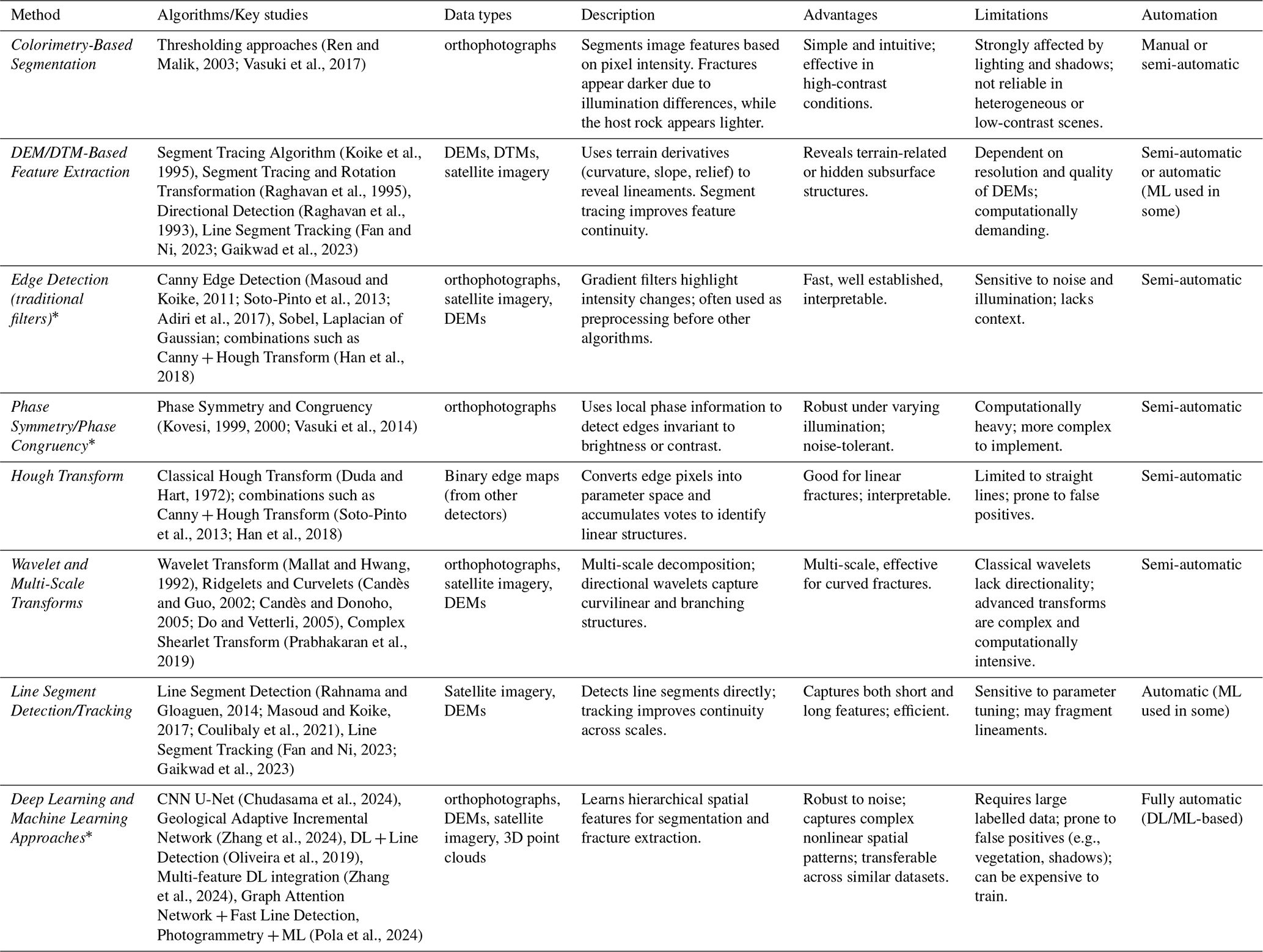
^∗ evaluated in this study.

These challenges motivate faster, more reproducible fracture-tracing methods. Rapid advances in computer vision and machine learning (ML) have made automated fracture detection an appealing alternative to manual and semi-automated methods (Thiele et al., 2017b; Mattéo et al., 2021; Chudasama et al., 2024). Various techniques have been developed for fracture detection from orthophotographs (including satellite imagery), digital elevation models (DEMs), and digital terrain models (DTMs). These techniques range from classical image processing methods, including colorimetry-based segmentation, edge detection, phase symmetry and phase congruency, and Hough transforms, to more advanced deep learning (DL) approaches (Table 1). Each method has benefits and limitations that depend on data type and image quality.

Among the classical approaches, colorimetry-based segmentation exploits the contrast between fractures and host rock but is highly sensitive to lighting and shadowing (Ren and Malik, 2003; Vasuki et al., 2017). DEM and DTM-based feature extraction methods, such as segment tracing and directional detection algorithms (Koike et al., 1995; Raghavan et al., 1993, 1995), can reveal terrain-related structures but depend heavily on the resolution and quality of the underlying elevation data and are computationally demanding. Edge-detection filters (e.g., Canny, Sobel, Laplacian of Gaussian) are fast and well-established but are sensitive to noise and provide no contextual information about what they detect (Masoud and Koike, 2011; Soto-Pinto et al., 2013; Adiri et al., 2017). Phase symmetry and phase congruency methods improve robustness to variable illumination (Kovesi, 1999, 2000; Vasuki et al., 2014), though at greater computational cost, while the Hough transform is effective for identifying straight linear features but is intrinsically limited to linear geometries and prone to false positives (Duda and Hart, 1972). Wavelet and multi-scale transforms (Mallat and Hwang, 1992; Candès and Guo, 2002; Candès and Donoho, 2005; Do and Vetterli, 2005; Prabhakaran et al., 2019) improve the handling of curvilinear, multi-scale features, although classical wavelets lack directionality. Dedicated line-segment detection and tracking algorithms (Rahnama and Gloaguen, 2014; Masoud and Koike, 2017; Coulibaly et al., 2021; Fan and Ni, 2023; Gaikwad et al., 2023) offer a complementary approach for capturing such features. Their more advanced variants are complex to implement, and line-tracking approaches remain sensitive to parameter tuning and prone to fragmenting continuous lineaments. A common shortcoming is reliance on hand-crafted rules and fixed-scale filters, which limits robustness to variable image quality (lighting, weathering, vegetation) and resolution typical of natural outcrop imagery, and constrains generalisation across datasets (Aghaee et al., 2021).

Deep learning and machine learning approaches form a distinct, rapidly growing category. These include convolutional neural network architectures such as U-Net for pixel-wise fracture segmentation (Chudasama et al., 2024), incrementally trained networks designed to adapt to new geological settings such as the Geological Adaptive Incremental Network (Zhang et al., 2024), hybrid approaches that combine DL-based feature extraction with classical line detection (Oliveira et al., 2019), multi-feature DL integration strategies that combine several input modalities (Zhang et al., 2024), and combinations of graph attention networks with fast line detection algorithms. DL methods have also been applied directly to 3D data, for example by coupling photogrammetric reconstruction with ML-based fracture extraction (Pola et al., 2024).

The main drawbacks of DL and ML approaches are reliance on large labelled training sets, their tendency to produce false positives in the presence of vegetation, shadows, and other artefacts, and the computational expense of training (An et al., 2023; Yaqoob et al., 2024; Mattéo et al., 2021; LeCun et al., 2015). Despite these disadvantages, DL and ML approaches offer clear advantages over classical methods: they are more robust to noise, can capture complex non-linear spatial patterns inherent to fracture networks, and once trained are commonly transferable across similar datasets (Mattéo et al., 2021; Chudasama et al., 2024; LeCun et al., 2015).

The key advantage of deep learning over classical feature extraction (Table 1) is learning spatial features directly from data at multiple scales simultaneously, rather than relying on hand-crafted rules and fixed-scale filters (LeCun et al., 2015). This is especially valuable for fracture mapping because fractures are inherently multi-scale, ranging from microfractures that are only visible in thin section to fault systems spanning tens, hundreds, or even thousands of meters in length. Furthermore, fractures normally present as sets or networks rather than isolated features. Learning various representations of fracture networks across scales allows a model to combine fine-scale edge detail with broader-scale network context, helping it distinguish fracture geometry from noise and other “edges” common in orthophotographs, such as vegetation boundaries, shadows, and weathering features.

Several issues still need to be addressed as DL-based automated fracture detection continues to develop. First, these methods still struggle with false positives and negatives, particularly under natural and uncontrolled imaging conditions (e.g., white balance, illumination patterns, resolution, etc.) (Mattéo et al., 2021; Yaqoob et al., 2024; An et al., 2023), e.g., topographic shadows mimicking fracture traces, vegetation creating false linear features, or weathering textures producing edges indistinguishable from fractures. Natural outcrops contain shadows, vegetation, uneven lighting, and erosional features, all of which can confuse detection algorithms. Second, fractures are an unusual target for semantic segmentation, as they are better represented as linear segments with arbitrary widths (Fig. 1a) rather than as continuous areas (Fig. 1b). Third, ground-truth labels used for training are often drawn at a coarser scale than the maximum image resolution allows: a time-saving compromise that leads to misalignment between the labelled fracture and the pixels that represent the fracture in the orthophotograph (Fig. 1c and d). While these inconsistencies may influence analyses of fracture lengths, orientations, and network topology, they have an even greater impact on model training and evaluation accuracy. This is important because annotation scale and interpretation can significantly affect the derived properties of fracture networks (Peacock and Sanderson, 2026). Finally, algorithm performance commonly drops when a DL-based model is applied to new datasets with different fracture patterns, lithologies, topographical complexity, or imaging conditions, limiting generalisability (Mattéo et al., 2021).

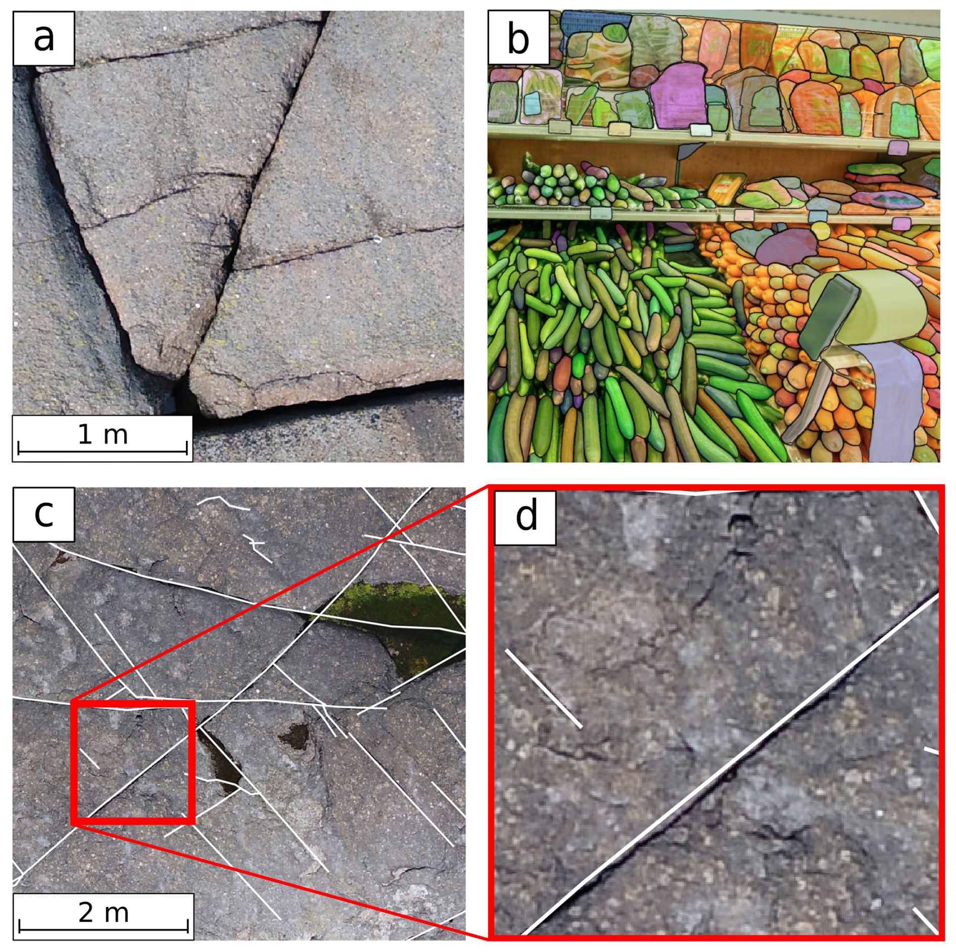
Figure 1 Example of annotation misalignment. (a) Example of fractures of different widths. (b) Example of a segmentation task represented as a continuous area from Segment Anything paper (Kirillov et al., 2023). (c) Outcrop orthophotograph (Nordbäck and Ovaskainen, 2025) overlaid with fracture traces in white from the ground-truth labels (Ovaskainen and Nordbäck, 2022). (d) Zoomed-in view showing how manually drawn fracture lines deviate from the actual visible fracture edges.

As automated fracture detection advances, there is an urgent need for standardised benchmarking frameworks and shared datasets that enable consistent and fair comparison of methods (An et al., 2023). While initiatives like GeoCrack (Yaqoob et al., 2024), a publicly available benchmark dataset for automated geological fracture detection in RGB images of rock outcrops, has begun to address this gap, current resources remain limited to RGB imagery and predominantly vertical outcrops and contain incomplete annotations in some image patches where only a subset of visible fractures are labelled.

The primary goal of this study is to establish a standardised evaluation framework for pixel-wise fracture segmentation from 2D outcrop imagery, using both traditional computer vision and deep learning methods. We present FraXet, comprising three curated, heterogeneous benchmark datasets on which a suite of traditional image-processing filters (Canny, Sobel, Gabor, Sato, and phase congruency) and deep learning models (U-Net, SegFormer) were applied to generate per-pixel fracture probability maps. The performance of the different methods was assessed using image-quality metrics (e.g., MSE, PSNR), segmentation metrics (e.g., precision, F1-score, IoU), and a novel fracture-trace similarity metric. By applying consistent preprocessing, hyperparameter optimisation, and evaluation metrics, our framework enables systematic comparison of fracture detection performance across diverse datasets, geological settings, and imaging conditions. FraXet is intended as a living benchmark, to be expanded with additional datasets representing different geological settings, lithologies, and fracture network patterns as more annotated public datasets become available. Our aim is to promote transparency, reproducibility, and comparability in automated fracture mapping research, while providing a useful test dataset and benchmark for future developments.

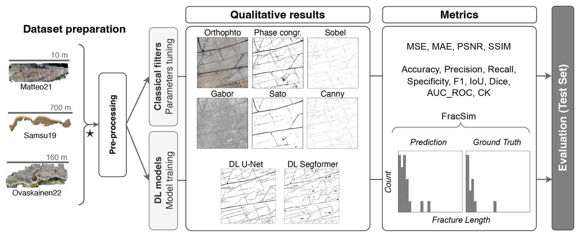
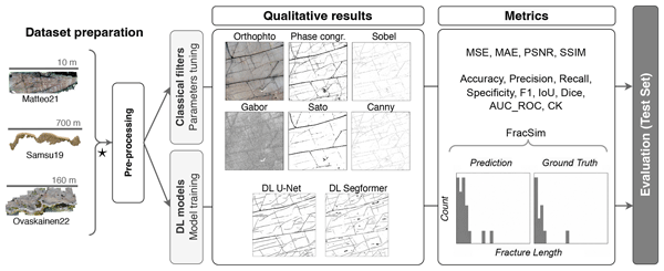
Figure 2 Overview of the benchmarking workflow. The three datasets (Matteo21, Samsu19, Ovaskainen22) are processed into the FraXet v0.1 database, used to train classical filters and deep learning models, the results of which are evaluated on the test set through qualitative visualisation and quantitative metrics and proposed similarity metric. ⋆: not all outcrops used shown here. Detailed dataset overviews are provided in Appendix (Figs. A1, A2, A3).

2 Methodology

We designed a benchmarking workflow (Fig. 2) for three publicly available, annotated outcrop datasets (Ovaskainen22 (Nordbäck and Ovaskainen, 2025; Ovaskainen and Nordbäck, 2022), Matteo21 (Mattéo et al., 2020), and Samsu19 (Samsu et al., 2019)) that make up the first version of FraXet (Fatihi et al., 2025a). FraXet is a curated benchmark dataset for training and evaluating automatic fracture-trace extraction models, comprising high-resolution orthophotographs and DEMs across diverse lithologies and outcrop geometries.

From the original orthophotographs and DEMs, we compiled 8953 co-registered 256 pixel × 256 pixel patches (see Fig. 3), each consisting of an RGB orthomosaic tile, a DEM tile, and a corresponding binary 1-pixel-wide fracture label. We standardised and pre-processed all the patches, then applied a suite of traditional image-processing filters (Canny, Sobel, Gabor, Sato, phase congruency) and deep learning models (U-Net, SegFormer) to generate per-pixel fracture probability maps. All methods were evaluated using a set of image quality, segmentation, and proposed similarity metrics on held-out test splits, with deep models tuned on validation subsets before final testing.

Figure 3 Example RGB–DEM–label patches from FraXet.

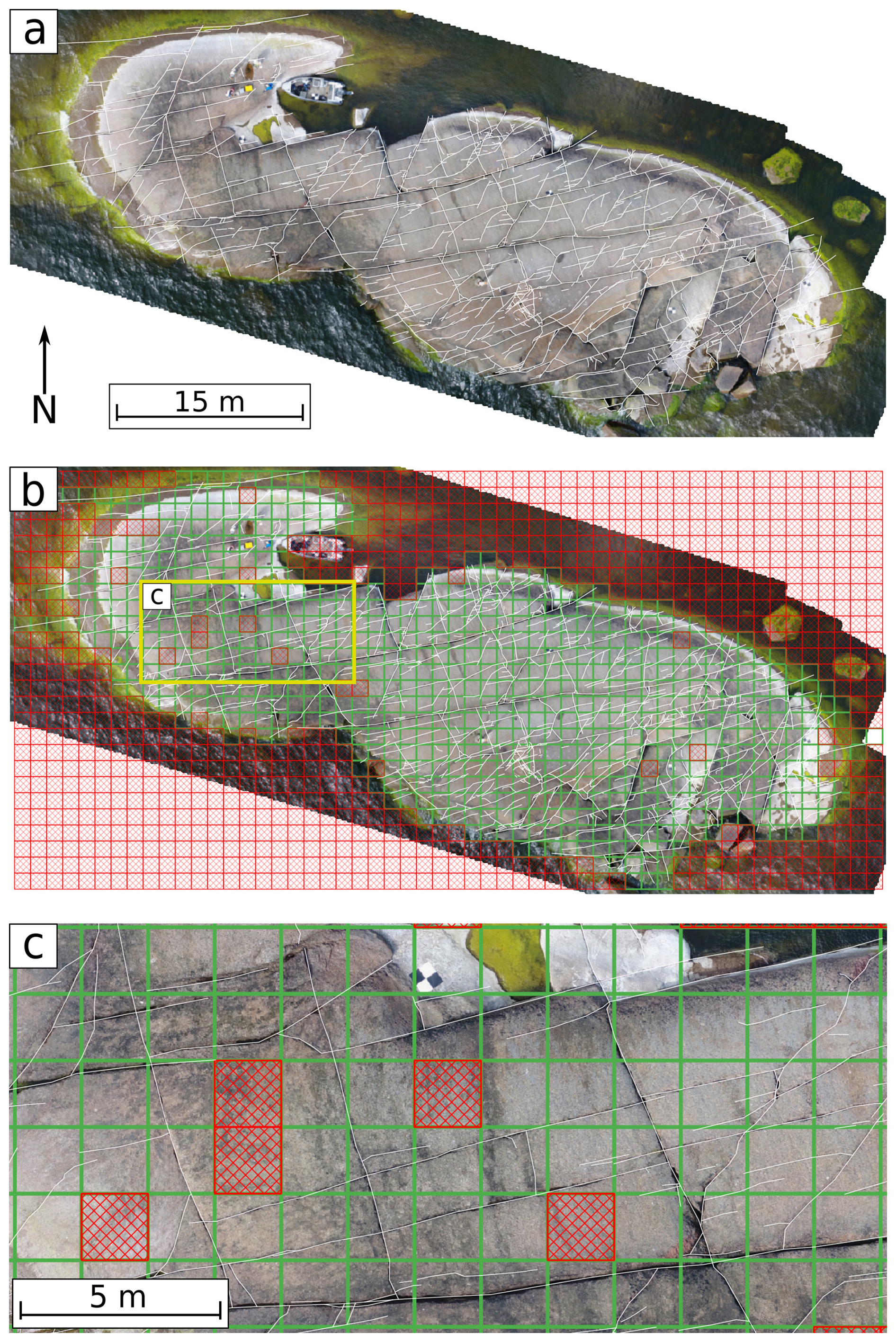
Table 2 Overview of datasets and their metadata and split statistics. Ovaskainen22: Nordbäck and Ovaskainen (2025) and Ovaskainen and Nordbäck (2022); Matteo21: Mattéo et al. (2020); Samsu19: Samsu et al. (2019).

^∗ As shared by the authors, no fixed mapping scale was used for fracture interpretation. Instead, fractures were digitised at the full image resolution (approximately 0.0055 m pixel size for data acquired from a 20 m drone flight altitude), allowing the interpreter to zoom freely as needed. Based on the image resolution, the effective fracture extraction scale is approximately 1:10 as in Ovaskainen et al. (2023).

2.1 Data Compilation

2.1.1 Data description

Ovaskainen22 captures fracture networks in the Mesoproterozoic Wiborg Rapakivi Granite Batholith of southeastern Finland, mostly isotropic coarse-grained wiborgite-facies granite with K-feldspar megacrystals up to 5–10 cm (Härmä, 2020). Matteo21 (Mattéo et al., 2021) presents data from the Granite Dells, Arizona, an anorogenic granite of similar age (∼ 1.40 Ga) but with medium-grained, generally equigranular textures showing weak porphyritic tendencies (Krieger, 1965). Samsu19 (Samsu et al., 2019) maps fractures in a very different geological setting: a fluvial–lacustrine syn-rift sediment succession in the Lower Cretaceous Strzelecki Group (southeastern Australia), comprising mud- and sand-dominated siliciclastic strata with conglomeratic or organic-rich interbeds (Constantine, 2001).

Together, these three datasets cover varied geological contexts (from isotropic crystalline to anisotropic sedimentary lithologies) with fractures mapped at different scales, providing a diverse testbed for evaluating model generalisation. An overview of the datasets, their mapping scales, original study purposes, their resolutions, and split statistics is provided in Table 2. For completeness, overview maps of the sites used in this study are provided in the Appendix (Figs. A1, A2, A3).

We acknowledge that three datasets covering two granite types and one clastic sedimentary setting, while providing meaningful lithological contrast for a first benchmark, do not represent the full diversity of geological settings encountered in practice; notably absent are carbonate, metamorphic, and volcanic lithologies. FraXet is intended as a living benchmark to be expanded as further annotated public datasets become available; including these other lithological settings is a priority for future work.

In addition, a single site from the Lapiés di Bou karst surface was included to enable qualitative visual comparison across methods. This locality lies within the Helvetic domain of the Swiss Western Alps, specifically within the Wildhorn Nappe complex (Steck et al., 2001; swisstopo, 2024), where fine limestones to marls, locally oolitic, of the Aptian–Barremian Schrattenkalk Formation crop out (Badoux et al., 1959). Two patches from the Bingie Bingie area were also used for the timing experiment, allowing direct comparison with the manual and semi-automatic mapping workflow of Thiele et al. (2017a). Neither the Lapiés di Bou nor the Bingie Bingie data were included in the training, validation, or test splits; they were used exclusively for qualitative visual comparison and runtime evaluation, respectively.

2.1.2 Test, train and validation splits

To ensure reliable model assessment and minimise spatial autocorrelation – a known issue in geospatial machine learning where spatial overlap inflates accuracy metrics by reducing the statistical independence of training and testing data (Wang et al., 2023) – we have defined spatially disjoint data splits by dividing each of the three datasets into training, validation, and test regions (with no spatial overlap). Specifically, here the Ovaskainen22 dataset consists of Orrengrund (training), Kasaberget (validation), and Kampuslandet (testing) islands off the coast of the Loviisa region; the Samsu19 dataset comprises Eagles Nest (training) and Harmers Haven north (split between validation and testing); and the Matteo21 dataset is split into sites A and B (training), held-out regions of A and B (validation), and site C (testing). Only tiles containing at least one labelled fracture pixel were retained, to reduce challenges with class imbalance and to focus learning on relevant features.

The orthophotographs and DEMs were resampled to have matching spatial resolution, normalised, and tiled into non-overlapping 256 pixel × 256 pixel patches, each with four channels (RGB + DEM). This patch size balances field of view, feature scale, and computational efficiency: it is large enough to preserve contextual information while remaining compatible with typical convolutional neural network (CNN) input constraints.

Ground truth annotations for Ovaskainen22 and Samsu19 were provided as vector shapefiles and were subsequently rasterised to the corresponding image resolution, producing binary masks with 1-pixel-wide white fracture lines on a black background. These binary images match the raster-formatted annotations in Matteo21 to ensure consistent label representation.

Given the spatial resolutions of the datasets, a 256 pixel × 256 pixel patch represents a square region with side lengths ranging from approximately 0.13–0.33 m (Matteo21), 1.28–1.54 m (Ovaskainen22), and 7.4–8.2 m (Samsu19).

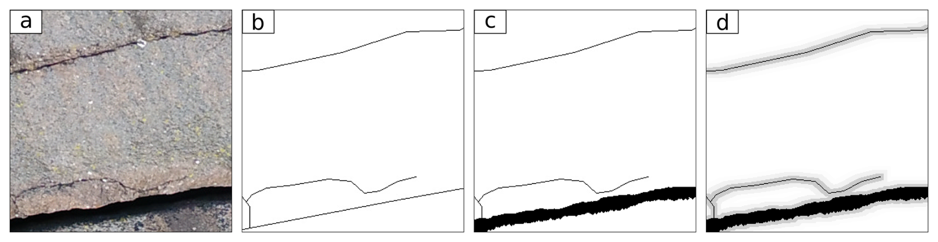
Figure 4 Label refinement steps. (a) Original RGB image; (b) manually traced ground truth with 1-pixel-wide fractures; (c) widened annotations after region-growing; (d) smoothed probabilistic labels produced by multi-scale dilation.

Probability Map Representation. Because our goal is to generate per-pixel probability maps rather than hard binary labels, we designed all preprocessing steps with this output in mind. Probability maps provide a continuous estimate (0–1) of the likelihood that each pixel corresponds to a fracture, capturing confidence and uncertainty rather than forcing discrete predictions. This representation is well suited to fracture mapping, where annotations are often noisy or slightly misaligned, and where soft boundaries reflect the inherent ambiguity of thin linear features.

It also enables flexible post-processing: thresholds can be adjusted to balance precision and recall, high-confidence regions can be skeletonised to extract fracture traces, and outputs can be integrated into human-in-the-loop workflows or combined with traditional filters. Moreover, probability maps support richer evaluation metrics (e.g., ROC analysis), and improve robustness when using ensembles or multi-scale fusion. For all these reasons, probability maps serve as the most informative and practical output of the methods.

2.2 Pre-processing

Several preprocessing and augmentation steps were applied prior to model training and evaluation, to standardise inputs, refine ground-truth annotations, and improve model generalisation. All preprocessing scripts and procedures are publicly released as the FraXtex2D gitlab repository (https://gitlab.com/ayoubft/fractex2D.pt, last access: 14 September 2026) to ensure reproducibility. These procedures are summarised below.

Depth. For all deep learning experiments, we used the full RGB imagery together with the corresponding DEM channel, which was normalised at the patch level using min–max normalisation. This scaling ensures that elevation values within each patch fall between 0 and 1, reducing the influence of absolute elevation differences across sites and improving numerical stability during training.

Channel selection. Most traditional edge-detection filters operate on a single image band. Therefore, each band was first z-standardised (zero mean, unit variance) on the patch-level to reduce sensitivity to illumination differences and overall brightness. PCA (principal component analysis) was then applied to the normalised four-band data to obtain a single-band representation containing a maximal amount of variance.

Label refinement. We implemented two complementary label-processing techniques to correct inconsistencies in the original fracture annotations and enhance their spatial accuracy: wide-fracture expansion and multi-scale label smoothing.

Wide-fracture expansion. Preliminary experiments revealed that the models underperformed on wide, visually prominent fractures. Many such fractures were annotated as 1-pixel-wide lines, underrepresenting their true width. To address this, we developed a region-growing algorithm that widens single-pixel annotations to fill thick fracture zones. This algorithm (Fig. 4c) fills dark linear regions in the green channel, identified by thresholding at 30 (on a 0–255 scale), by applying a 2-pixel maximum filter, followed by morphological dilation, then merging the resulting dark, connected regions with the original binary mask. Only expanded areas connected to existing labelled pixels are retained to prevent false positives. This operation improved annotation fidelity for wide fractures.

Multi-scale label smoothing. Manual fracture tracing also often introduces small misalignments between annotations and actual fracture pixels, especially in high-resolution orthophotographs. First, labels are expanded with a distance of 2 pixels to fill small gaps and buffer the reference traces. This is followed by three successive morphological dilations applied to the expanded mask using disk-shaped structuring elements with radii of 2, 5, and 7 pixels. These bands are then combined into a graded representation using decreasing weights of $\frac{\mathrm{1}}{\mathrm{3}}$, $\frac{\mathrm{1}}{\mathrm{5}}$, and $\frac{\mathrm{1}}{\mathrm{9}}$, respectively. This produces a smooth boundary around fractures (Fig. 4d). This approach reduces sensitivity to annotation noise and improves training stability by explicitly modelling spatial uncertainty.

Together, these two steps improved correspondence between fracture labels and actual image structures, increasing the effective proportion of positive (fracture) pixels and slightly reducing class imbalance (Table B1 in the Appendix).

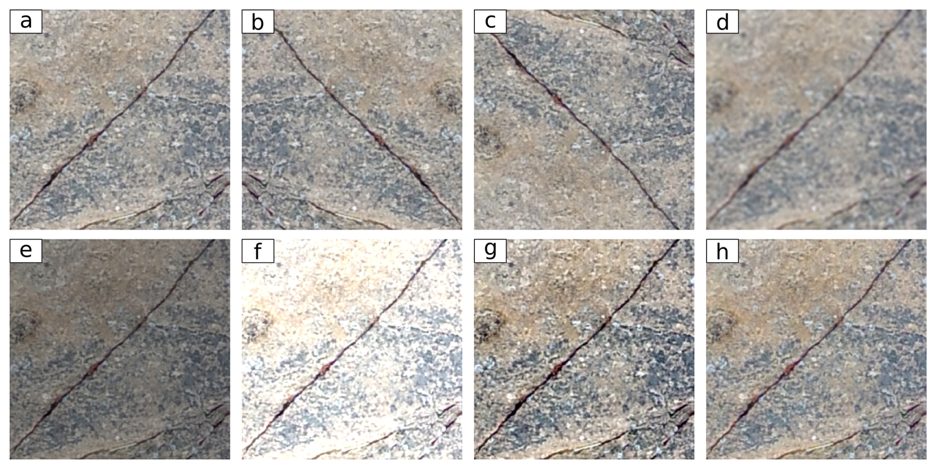
Figure 5 Data augmentations applied during training: (a) original, (b) horizontal flip, (c) vertical flip, (d) gaussian blur, (e) brightness decrease, (f) brightness increase, (g) contrast increase, (h) saturation increase.

2.3 Data augmentation

To further enhance model robustness and generalisation, we applied the following data transformations randomly to the input patches (Fig. 5) during each training epoch:

• 1.

  Flipping horizontally and vertically. These transformations are applied to both the RGB + D images and the ground truth labels to encourage geometric invariance, helping the model detect fractures regardless of their orientation.

• 2.

  Gaussian blurring, brightness, contrast, and saturation adjustment. These are applied only to the RGB channels to promote photometric invariance, improving robustness to changes in lighting and appearance. Table C1 in the Appendix summarises the applied augmentations and their parameters.

2.4 Image filter-based approaches

This section outlines our implementation of several established image-processing filters as a baseline for comparing deep learning results. These methods do not require training data and operate directly on the image, offering fast, interpretable, and reproducible outputs. While not specifically designed for fracture detection, they are widely used in geoscientific and remote sensing applications to extract features with similar morphology. All filters were applied to the first principal component (channel) resulting from the PCA reduction.

For the classical filters, which do not produce probabilistic outputs, we applied the same label-dilation step (Step 2 in preprocessing; Sect. 2.2) to their binary masks. This ensures that all methods are evaluated against labels that better reflect the actual fracture width and account for the misalignment between annotations and true pixel-level fracture geometry observed earlier.

We grouped the filters into three main categories, also see Table 1:

• Edge detection (Sobel and Canny): Computes spatial intensity gradients to highlight abrupt changes. These filters are simple and efficient but sensitive to noise and lighting, and some require thresholding to generate binary edges.

• Ridge detection (Gabor and Sato): Identifies elongated, linear structures by analysing second-order derivatives (curvature). These filters can capture fracture-like ridges at tuned scales but may also respond to non-fracture textures.

• Phase-based filters (Congruency): Use Fourier phase information to detect edges. These methods handle varying illumination more robustly, but are computationally intensive and involve more tunable parameters.

Table 3 Summary of parameters adjusted for each algorithm and their descriptions.

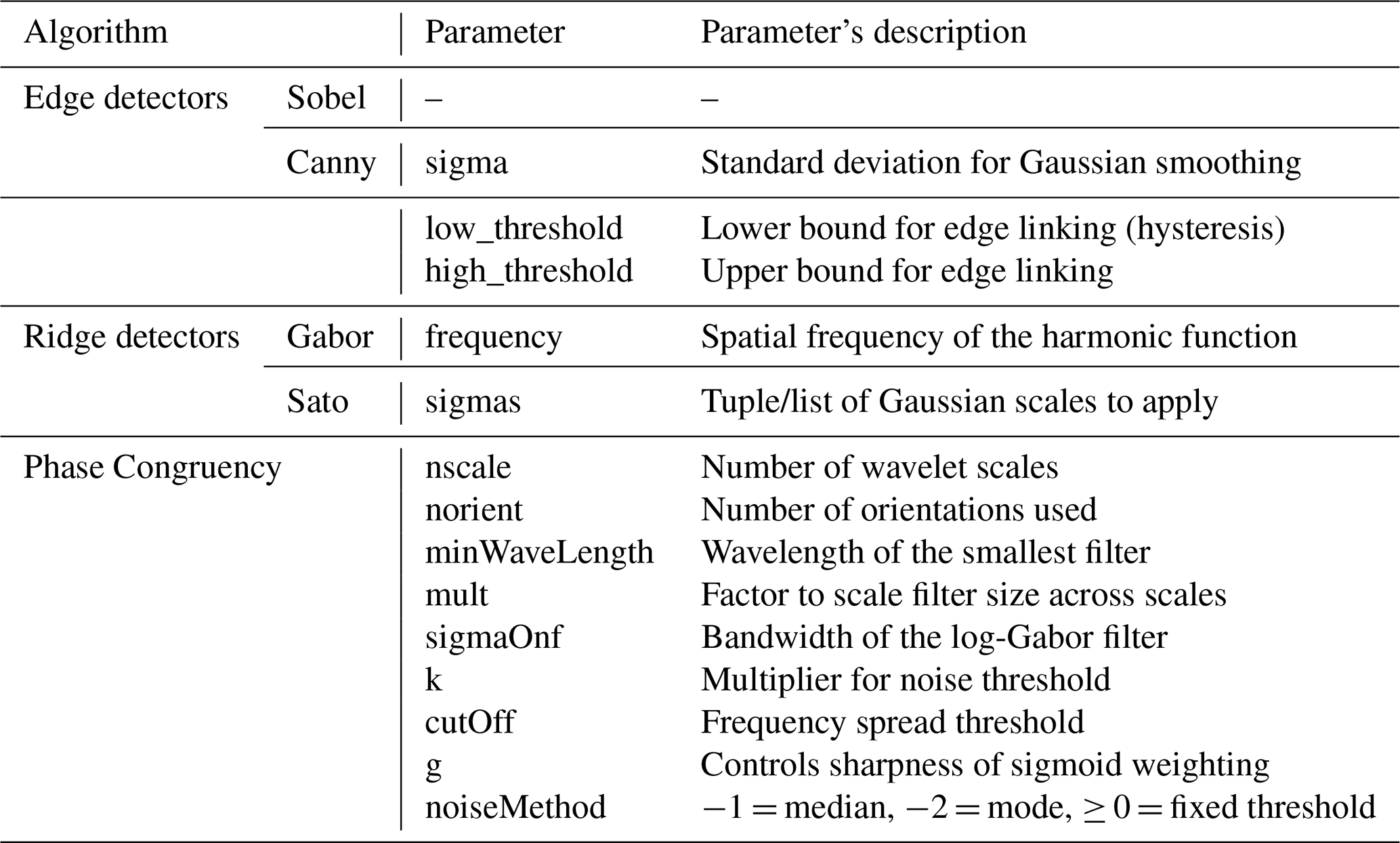
Each of these methods relies on user-specified parameters (Table 3; Sect. 2.4.1) to suppress background clutter and isolate relevant target features (fractures in our case).

2.4.1 Parameter Selection

To explore the behavior of each filter across different datasets, we first conducted a manual visual tuning phase. This provided insight into which parameter settings produced plausible results and helped define sensible parameter ranges. We then applied a data-driven parameter search to select the optimal settings for each filter. Specifically, we performed a grid search with cross-validation, which is justified here due to the low dimensionality of the parameter space and the relatively small number of candidate values per method. For each configuration within the predefined parameter ranges, the filter response was dilated (Step 2 in preprocessing), thresholded, and evaluated against the refined ground truth using the F1 score (defined in Table 4). The parameter set yielding the highest score was selected as optimal. This grid search standardises filter hyperparameters across datasets and reduces subjectivity in parameter selection.

2.5 Deep Learning-Based Models

Two deep learning architectures are evaluated in this work: a convolutional U-Net (Ronneberger et al., 2015) and a transformer-based SegFormer (Xie et al., 2021), the latter initialised with pretrained ResNet34 weights as its backbone. U-Net is widely used for semantic segmentation due to its encoder-decoder architecture and skip connections, while SegFormer leverages attention mechanisms combined with the ResNet34 backbone for long-range context modelling and robustness to geometric variability.

Both models were trained with architecture-specific hyperparameters selected by cross-validation and sensitivity tests. For the U-Net, we used the Adam optimiser with an initial learning rate of 0.05, while the SegFormer employed RMSProp with an initial learning rate of 0.01. The input to each model consisted of 256 pixel × 256 pixel patches with four channels (three RGB bands and one DEM band). We used Huber (smooth L1) loss for per-pixel probability targets, as it proved robust to label noise, spatial misalignment, and class imbalance compared to binary cross-entropy or Dice loss (both popular for segmentation tasks). Early stopping based on validation loss was used in both cases to prevent overfitting.

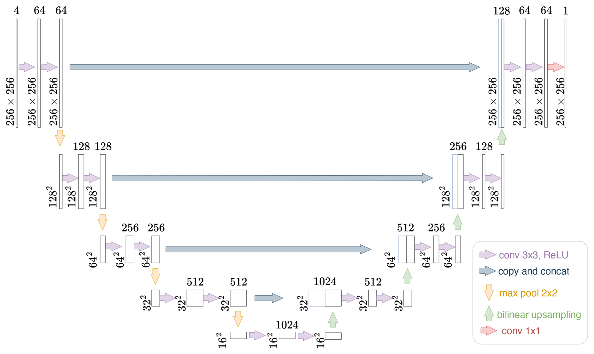
Figure 6 Overview of the U-Net encoder–decoder architecture with skip connections (Ronneberger et al., 2015). The encoder (left) progressively downsamples the 256 × 256 × 4 input through convolutional blocks (Conv → BatchNorm → ReLU) and max-pooling, extracting features at multiple scales. The decoder (right) upsamples these features via transposed convolutions and concatenates them with the corresponding encoder features via skip connections (grey arrows), preserving spatial detail. The final 1 × 1 convolution produces a per-pixel fracture probability map.

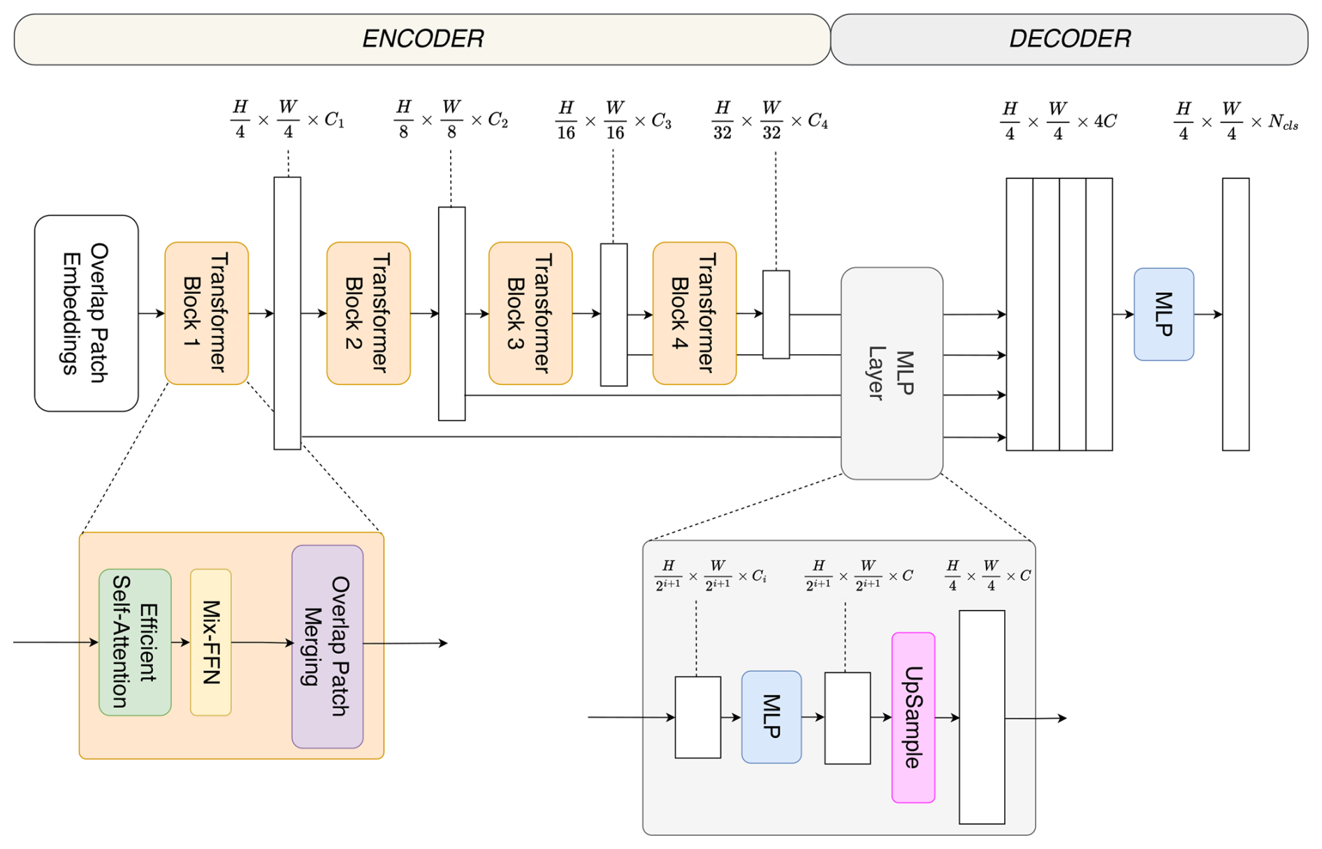
Figure 7 Overview of the SegFormer architecture combining a transformer encoder with a lightweight decoder (Xie et al., 2021). The encoder uses a hierarchical transformer backbone (ResNet34) with multi-head self-attention to capture long-range dependencies. The decoder aggregates multi-level features via a simple MLP. Terms: Self-attention: mechanism allowing each pixel to attend to all others; MLP: multi-layer perceptron; Feature map: spatial representation at each encoder stage.

The U-Net and SegFormer architectures are depicted in Figs. 6 and 7, respectively.

Both models produce per-pixel probability maps used for visual comparison and were thresholded to generate binary segmentation masks, which were then compared to the ground truth using the metrics described below.

2.6 Benchmark metrics

To evaluate segmentation performance, we used three complementary groups of metrics:

1. image-quality metrics that quantify how closely the predicted probability maps match the annotated targets,

2. pixel-wise classification and segmentation metrics that measure detection performance and spatial overlap, and

3. a proposed fracture-level similarity metric, FracSim, designed to compare the geometry of predicted fracture traces with those in the ground truth.

Table 4 Overview of metrics for evaluating image quality and segmentation.

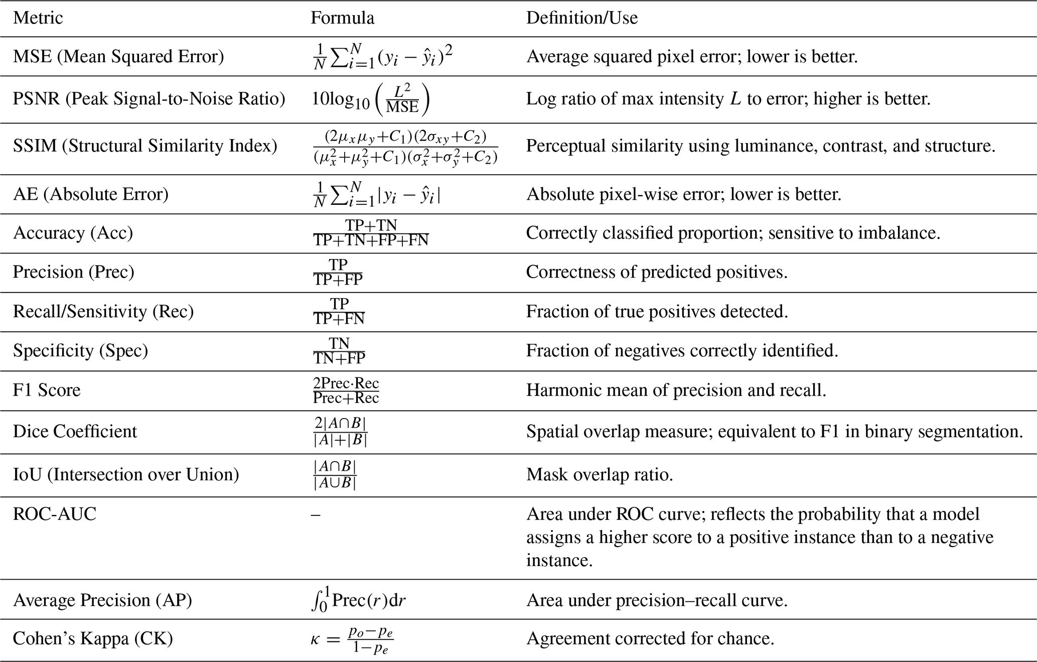
Symbols: N = number of pixels; y_i = reference pixel value; ${\widehat{y}}_i$ = predicted pixel value; L = maximum possible pixel intensity; μ_x,μ_y = means of image patches x and y; ${\mathit{\sigma }}_x^{\mathrm{2}},{\mathit{\sigma }}_y^{\mathrm{2}}$ = variances; σ_xy = covariance; C₁,C₂ = SSIM stability constants; $\text{TP},\text{TN},\text{FP},\text{FN}$ = true/false positives/negatives; A,B = predicted and reference binary masks; r = recall; p_o = observed agreement; p_e = expected chance agreement; ROC: receiver operating characteristic, is a graphical plot which illustrates the performance of a binary classifier system as its discrimination threshold is varied. ROC in Tables 5 and E1 and in Fig. 9 denotes ROC-AUC.

Together, these metrics (Table 4) capture prediction quality at the pixel, mask, and structural levels. Higher values generally indicate better performance, except for error metrics (MSE, AE), where lower values are preferable.

We include the background class in our evaluation to capture each model's full performance across the entire image. Because fractures represent only a very small fraction of pixels, excluding the background can artificially inflate metrics such as precision and recall. It also tends to make poorly calibrated models appear better, as ignoring the dominant class often results in models overpredicting fractures. Including the background therefore provides a more realistic assessment of false positives, calibration, and overall segmentation integrity. Notably, many previous studies do not explicitly report whether the background class is included in the computation of evaluation metrics.

Among the metrics computed, we consider the Dice coefficient (equivalent to the F1 score), recall, specificity, and intersection over union (IoU) as the most relevant for fracture segmentation. Accuracy, in contrast, is the least informative metric here: a model that predicts only background can achieve deceptively high scores due to class imbalance. Dice and IoU measure spatial overlap, which is critical for evaluating thin, linear features like fractures. Dice balances false positives and false negatives, while IoU penalises both over- and under-segmentation, making it a stricter metric. Recall ensures that fractures are not missed, while specificity quantifies how well the model avoids false positives in the dominant background class. Given the extreme class imbalance – background pixels can account for over 99 % of the image – reporting recall alone can be misleading. Specificity completes the picture by measuring the number of false detections in non-fracture regions.

We also include ROC-AUC, which evaluates the model's ability to distinguish between fracture and background pixels across thresholds. As a threshold-independent metric, ROC-AUC is particularly useful for probabilistic outputs. Similarly, Cohen's Kappa measures agreement between prediction and ground truth while accounting for chance, offering a more meaningful alternative to raw accuracy in imbalanced settings.

In addition to segmentation metrics, we report image-quality metrics – Mean Squared Error (MSE), Peak Signal-to-Noise Ratio (PSNR), Structural Similarity Index (SSIM), and Absolute Error (AE) – to assess how well the predicted probability maps match the annotations before thresholding. These metrics capture prediction fidelity in both intensity and structure. MSE and AE quantify raw pixel-wise error (lower is better), while PSNR measures signal degradation in a logarithmic scale (higher is better). SSIM accounts for human visual perception by evaluating structural and contrast similarity, which is especially valuable when preserving subtle linear patterns like fractures.

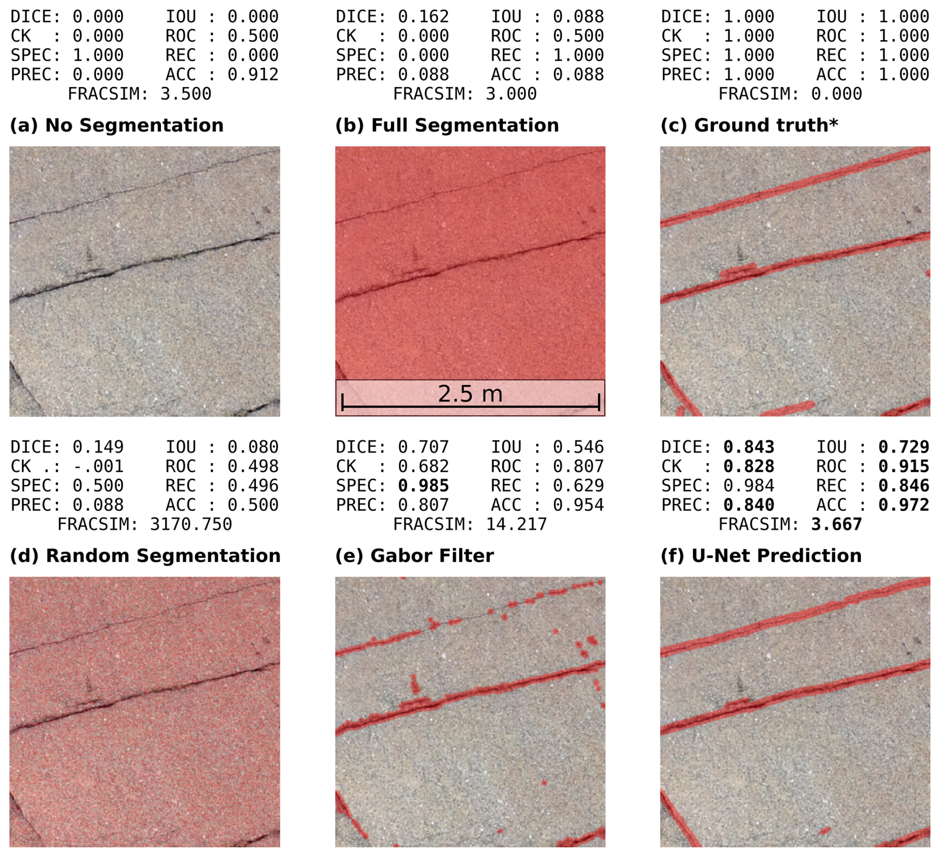
Figure 8 Illustration of metric behavior under different segmentation scenarios: (a) No segmentation (predicts all background), (b) Full segmentation (predicts all fracture), (c) Ground truth, (d) Random segmentation, (e) Gabor filter segmentation, (f) U-Net segmentation. Values in bold show the best scores, excluding scenarios a, b and c. Image from the Ovaskainen22, KL5 dataset. Abbreviations are defined in Table 4.

The different scenarios in Fig. 8 highlight how each metric responds to specific segmentation behaviors. Predicting only background (no segmentation) yields high accuracy and specificity but zero recall, precision, and overlap-based scores, illustrating how class imbalance can inflate accuracy despite complete failure to detect fractures. Conversely, full segmentation maximises recall while collapsing specificity and precision, resulting in low Dice and Intersection over Union values. Random segmentation produces near-chance values across most metrics, with Dice, Intersection over Union, Cohen's Kappa, and receiver operating characteristic scores reflecting the lack of spatial agreement. The Gabor filter segmentation shows intermediate performance, improving overlap, precision, and specificity by capturing some fracture structure, but still suffering from fragmentation and false positives. The U-Net prediction achieves the most balanced and consistently high scores across all metrics, with strong overlap, agreement, and classification performance, closely approaching the ground truth.

2.7 FracSim: a fracture-level similarity metric

Pixel-wise metrics are widely used for segmentation evaluation but have limitations when applied to thin, linear features such as fracture traces. Small differences in line thickness or slight spatial offsets can disproportionately affect precision, recall, and F1-score. For example, a correctly detected fracture predicted slightly thinner than the annotation will incur false negatives along its edges, substantially reducing recall despite successful detection.

To address these limitations, we developed FracSim, a domain-specific similarity metric that compares the distribution of extracted fracture segment lengths between the predicted mask and the ground truth.

For each prediction and label, we:

• 1.

  convert the probability map to a binary mask (user threshold, default: 0.1);

• 2.

  skeletonise the binary masks to a one-pixel wide trace;

• 3.

  remove short noisy junctions using a small neighborhood filter (to avoid counting cross-overs and thick junction blobs as segments);

• 4.

  label connected skeletal segments and compute their pixel lengths;

• 5.

  construct comparable histograms of segment lengths (same bin edges for prediction and ground truth); and

• 6.

  compute a symmetric chi-square distance between the two histograms (Eq. 1).

$$\begin{array}{}\text{(1)}& d_{{\mathit{\chi }}^{\mathrm{2}}}(h,g)={\displaystyle \frac{\mathrm{1}}{\mathrm{2}}}\sum _{i=\mathrm{1}}^N{\displaystyle \frac{(h_i-g_i{)}^{\mathrm{2}}}{h_i+g_i}}\end{array}$$

where

• $d_{{\mathit{\chi }}^{\mathrm{2}}}(h,g)$ is the symmetric chi-square distance between the two histograms,

• h and g are the two histograms being compared,

• h_i and g_i denote the values of the ith bin of histograms h and g, respectively,

• N is the total number of bins.

Lower χ² indicates closer agreement in the fracture length distribution. We compute FracSim only on patches that contain a high fracture-pixel count in the ground truth; empty or nearly empty patches are excluded because they lack a meaningful fracture-length distribution to compare, and even small prediction artifacts in these patches can otherwise produce misleading metric values.

Together, these metrics (Sects. 2.6 and 2.7) provide a balanced framework for evaluating both hard segmentation performance and the quality of soft probabilistic outputs.

2.8 Generalisation experiments

To evaluate the generalisation capability of a single model trained across diverse geological settings, we compared a multi-site model (trained on all datasets combined, M_all) against individual models trained separately on each dataset (M_ovas, M_sams, and M_matt). All models employed an identical architecture and training configuration, with no dataset-specific hyperparameter tuning conducted. Each dataset-specific model was evaluated only on its corresponding test set, while M_all was tested independently on each dataset. This experiment aims to assess whether a generalist model can match or exceed the performance of models trained under dataset-specific conditions, offering insights into the feasibility of cross-domain fracture segmentation.

3 Results

To assess performance, we evaluated traditional computer-vision filters and deep learning (DL) models on the held-out test set using the image-quality, segmentation, and similarity metrics described earlier. The following sections present qualitative and quantitative results.

3.1 Traditional Computer Vision–Based Algorithms

The optimal hyperparameters and thresholds that produced the best results, identified through grid search and manual visual inspection, are listed in Table D1.

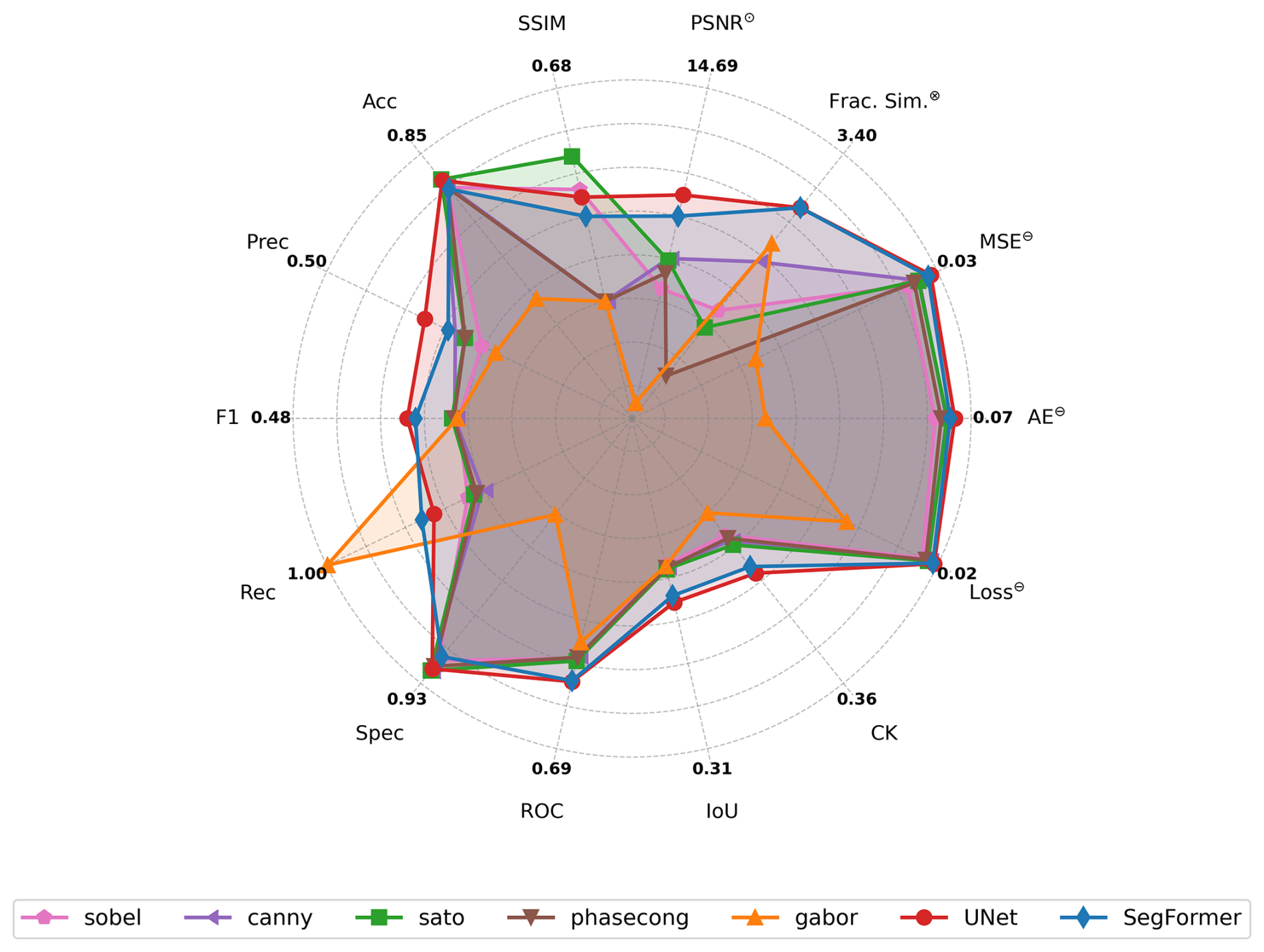
Figure 9 Radar chart summarising the performance of the classical filters and the deep learning models (U-Net, SegFormer) across all evaluation metrics. All metrics originally lie between 0 and 1, except PSNR^⊙ and FracSim^⊗. Metrics for which lower values indicate better performance (AE^⊖, MSE^⊖, Loss^⊖ and FracSim^⊗) were flipped by computing (1 – value) so that the chart consistently displays better performance toward the outer radius. FracSim^⊗ was calculated on the modified test set. Abbreviations are defined in Table 4.

3.1.1 Quantitative Results

For completeness, the full numerical results from both the grid-searched settings are provided in Table E1. The radar chart in Fig. 9 summarises how the traditional filters perform across image quality, segmentation, and similarity metrics. Overall, the filters cluster near the centre of the plot, indicating limited fracture-detection capability across metrics. Canny, Sobel, Sato, and Phase Congruency exhibit similar profiles, with modest accuracy, precision, F1, and IoU, and only small variations in recall, specificity, and ROC. For the structural similarity metric, they achieve an SSIM value of zero, indicating no structural similarity. In contrast, the error-based measures (MSE, AE, and loss) remain low, which is favorable. Gabor is the only method that diverges sharply from this pattern: it attains perfect recall but extremely low precision, yielding a highly unbalanced shape on the radar plot. Because it labels nearly all pixels as the fracture class, the remaining metrics collapse to very low values.

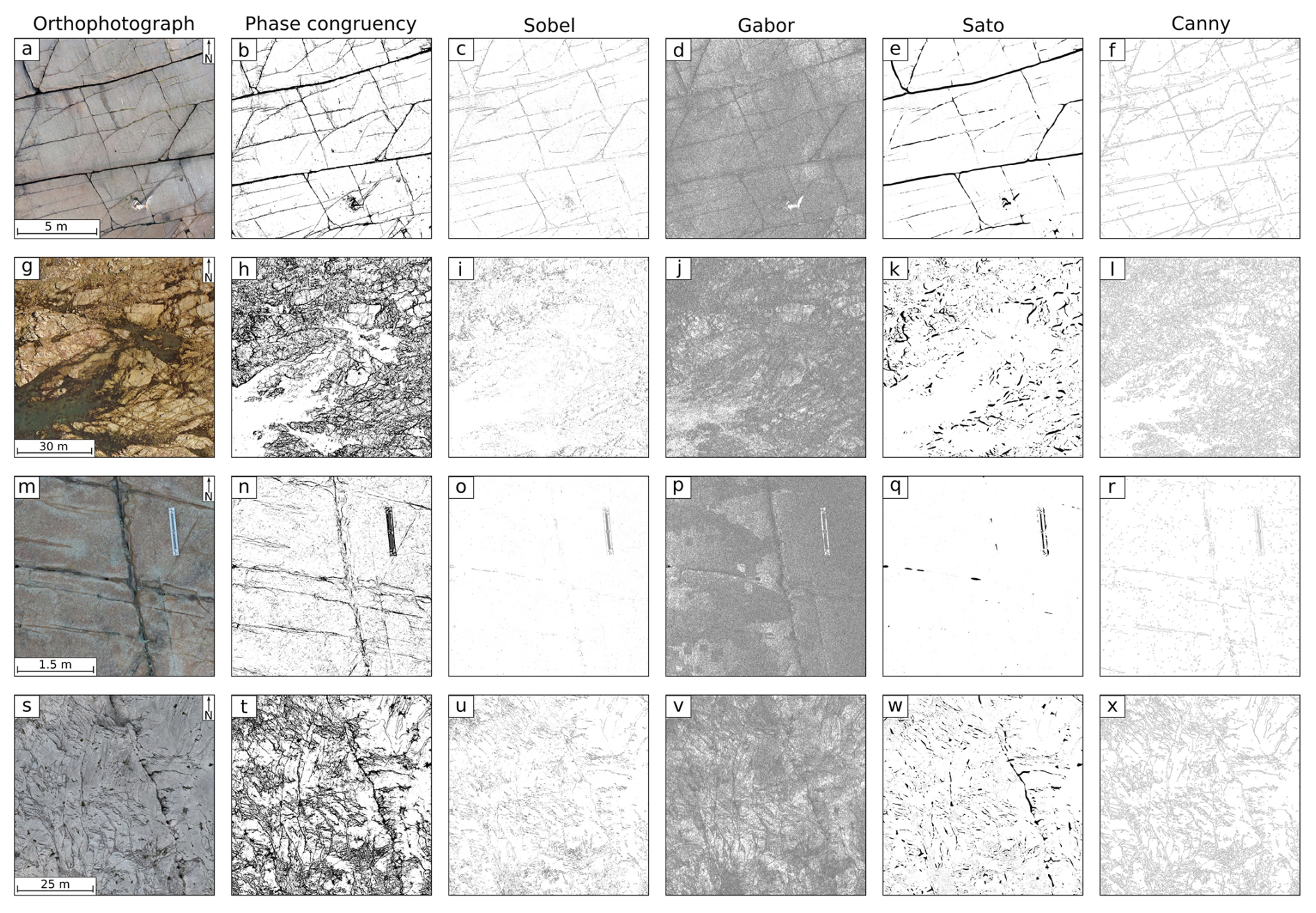
Figure 10 Comparison of traditional filters applied to four representative orthophotographs, using parameters selected by grid search. Each row shows an original orthophotograph (a, g, m, s) alongside results from Phase Congruency (b, h, n, t), Sobel (c, i, o, u), Gabor (d, j, p, v), Sato (e, k, q, w), and Canny (f, l, r, x) filters.

3.1.2 Qualitative Results

Using grid-searched parameters across all test sites, the classical filters produced partially useful but generally sparse outputs (Fig. 10). For example, in the Ovaskainen22 test patch (Fig. 10a–f), Phase Congruency (Fig. 10b) detected several fracture segments but introduced substantial noise, while Sato (Fig. 10e) captured only the most prominent ridges. In the Samsu19 patch (Fig. 10m–x), all filters struggled with the coarser resolution and sedimentary texture. Phase Congruency and Canny often highlighted many true fracture segments, but their responses included substantial noise and many thin lines. Sobel and Sato tended to be very sparse, picking up only the strongest edges or ridge cores, while Gabor largely failed to isolate fractures and instead responded to texture, producing noisy, non-fracture patterns. In short, the grid search showed that some filters can detect fracture signals, but universal parameter sets are not optimal for every site and yield noisy or incomplete maps.

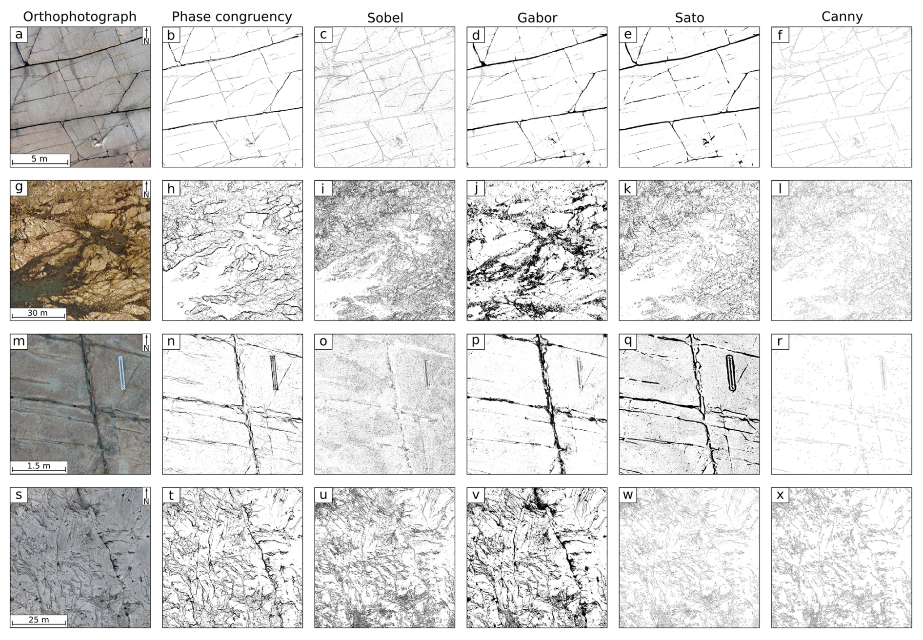
Figure 11 Comparison of traditional filters applied to four representative orthophotographs, using parameters selected manually for each site. Each row shows an original orthophotograph (a, g, m, s) alongside results from Phase Congruency (b, h, n, t), Sobel (c, i, o, u), Gabor (d, j, p, v), Sato (e, k, q, w), and Canny (f, l, r, x) filters.

Using manually tuned parameters on each test site separately, some filters were able to highlight fracture segments more clearly (Fig. 11). Sobel and Canny captured more pronounced edges along major traces, while Sato produced thicker and more continuous lines. However, the outputs also included numerous spurious detections of non-fracture features.

While manually tuned parameters can produce visually plausible outputs on individual test sites, this performance does not generalise well to other locations, or even to different regions within the same image. Traditional filters are sensitive to local contrast, scale, and texture, requiring site-specific adjustments to capture relevant features. These tuned parameters, although effective in isolated cases, often fail on heterogeneous datasets.

These limitations expose a core issue: fixed-rule and parameter-tuned traditional filters lack the flexibility to handle complex, real-world geological variability. They motivate deep learning approaches that do not rely on hand-crafted features or globally fixed parameters. Instead, they learn hierarchical representations directly from the data, enabling better adaptation to diverse fracture patterns and geological contexts. Deep networks can, in principle, generalise beyond specific sites by capturing shared structures across datasets.

Figure 12 Training and validation loss curves for U-Net and SegFormer (range: [0,1]).

3.2 Deep Learning Models

3.2.1 Training Dynamics

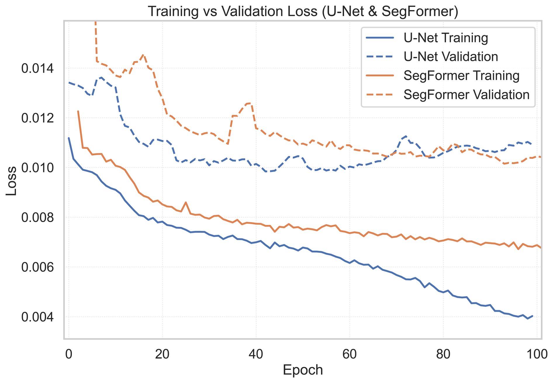
Model and hyperparameter selection was performed via cross-validation using the training and validation subsets. Figure 12 shows a representative training run for both architectures using the fixed hyperparameters described in Sect. 2.5 and a single random seed (42), ensuring that weight initialisation and other stochastic processes are reproducible across runs. The training curves illustrate the model learning process on the fracture datasets, showing how the segmentation error changes as the models learn to identify fracture patterns from the annotated RGB + DEM patches over successive epochs. The U-Net exhibits a smooth decrease in training loss and a validation curve that stabilises around epoch 43. The gap between the two curves remains small, with only mild overfitting toward the end of training. The checkpoint with the lowest validation loss was used for evaluation. SegFormer follows a similar downward trend but with higher loss values and more fluctuation, particularly during the first half of training. Its slower convergence suggests that the model adapts less effectively to this dataset than the U-Net, or alternatively, that it requires additional training data and longer training to achieve a comparable fit.

3.2.2 Quantitative Results

As shown in the spider diagram (Fig. 9) and Table E1, the U-Net model achieved a mean F1 score of 0.48 and IoU of 0.31, substantially higher than any traditional baseline (F1 < 0.29, IoU < 0.17). Precision reached 0.50 (half of the pixels predicted as fractures were true positives), while recall remained moderate (0.45), indicating missed fracture pixels. SSIM (0.49) and PSNR (14.7 dB) confirm that the reconstructed fracture masks deviate notably from the ground truth in terms of image similarity, yet the segmentation metrics demonstrate decent detection of fracture structures.

The SegFormer model was trained using the same data splits and evaluation protocol as the U-Net. While SegFormer produced competitive results, its F1 (0.44) and IoU (0.28) were consistently lower than those of the U-Net. Standard deviations across runs were similarly low, indicating stable but suboptimal convergence. Although the U-Net and SegFormer models clearly outperform filter-based methods, their absolute performance remains well below standard deep learning studies (F1 > 0.8, IoU > 0.6) (Guo, 2023; Kuş and Aydin, 2024; Sumi et al., 2024). This emphasises the challenging nature of fracture segmentation as a task and the relatively limited training data currently available.

Notably, the DL models (U-Net and SegFormer) achieve substantially lower FracSim (better agreement of length distributions) than classical filters. Thus DL predictions not only overlap ground truth spatially (IoU, F1) but also better reproduce fracture-segment length statistics.

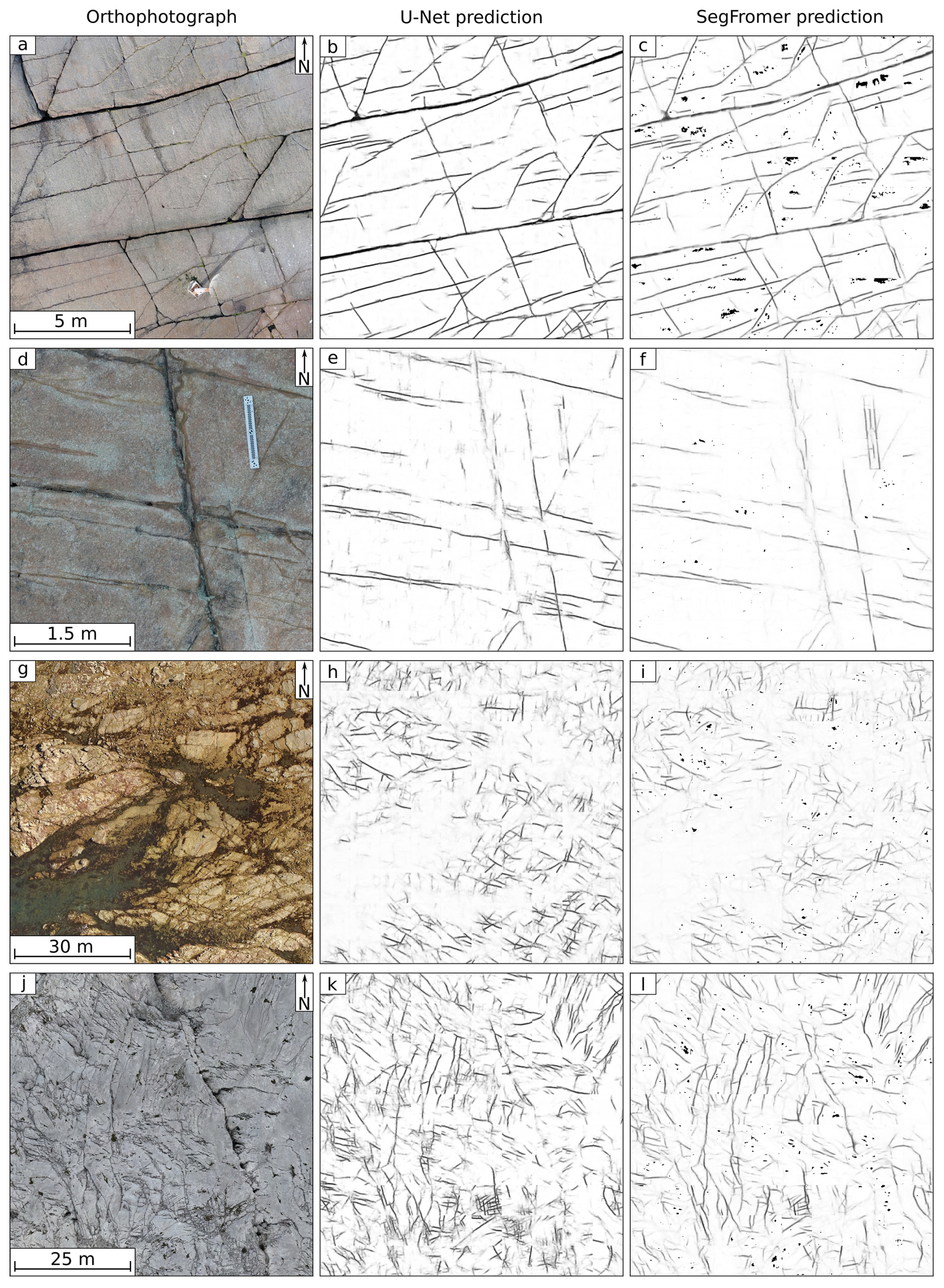
Figure 13 Deep-learning fracture-trace predictions for four representative orthophotographs, one per row. Each row shows the original orthophotograph (a, d, g, j) alongside the corresponding U-Net (b, e, h, k) and SegFormer (c, f, i, l) predictions.

3.2.3 Qualitative Results

Example outputs are shown in Fig. 13. Across the different datasets, the U-Net CNN consistently produced fracture maps that were smoother, more continuous, and closer to the ground-truth annotations than those from traditional filters. The model often reconnected segments that filters left broken, yielding fracture networks that were both cleaner and more interpretable. These improvements were observed even under varying lithologies and illumination conditions, consistent with the CNN's ability to generalise across a wide range of datasets. Remaining errors included omission of faint fractures and occasional short false positives in textured or shadowed areas. These qualitative results reinforce the quantitative findings: deep learning methods produce more reliable fracture maps than traditional filters, with notable improvements in continuity and interpretability across diverse geological settings.

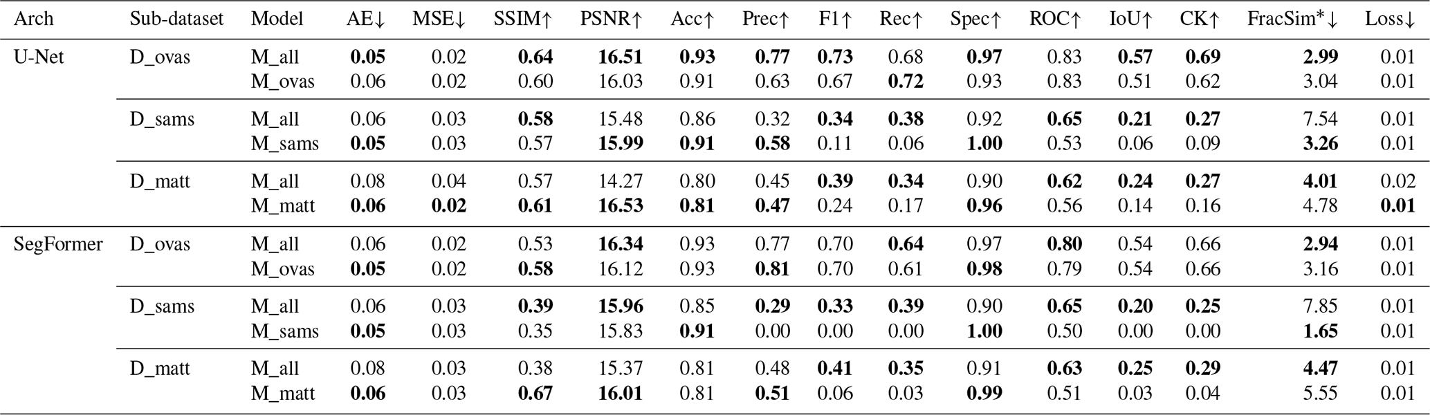
Table 5 Comparison between multi-site model (M_all) and dataset-specific models (M_ovas, M_sams, M_matt). Bold values indicate the better of the two models (M_all vs. the dataset-specific model) for each architecture, sub-dataset and metric; tied values are not highlighted.

^∗ run only on modified test set

Comparing the two deep learning models, SegFormer generated continuous predictions (Fig. 13) and sometimes captured long-range structures more effectively than U-Net. However, it introduced more false positives in complex textures, occasionally produced random hot spots, and overall yielded less confident and less precise outputs than U-Net across the test sites.

3.2.4 General vs. Dataset-Specific Models

Table 5 shows that the combined model (M_all) outperforms dataset-specific models, particularly in F1 and IoU.

On the D_ovas dataset, M_all and M_ovas exhibit comparable performance for both architectures. With U-Net, M_all achieves an F1-score of 0.73 and an IoU of 0.57, close to M_ovas (F1 = 0.67, IoU = 0.51); with SegFormer both models reach F1 = 0.70 and IoU = 0.54. This indicates that training on multiple datasets does not degrade performance on Ovaskainen22, where fractures are relatively clear and annotations are well defined.

The advantages of M_all become more pronounced on the more challenging sites. On D_sams, the site-specific model (M_sams) performs poorly, achieving very low scores (F1 = 0.11, IoU = 0.06 for U-Net; and zero for SegFormer) despite high specificity, indicating weak fracture identification relative to the ground truth. In contrast, M_all substantially improves performance, reaching F1-scores of 0.34/0.33 and IoU values of 0.21/0.20. This represents more than a twofold increase in overlap metrics, suggesting that the greater variability in the combined training set enables better generalisation to the more complex fracture patterns in the Samsu19 dataset.

A similar trend is observed for D_matt, where M_matt attains only F1 = 0.24 and IoU = 0.14 with U-Net (F1 = 0.06, IoU = 0.03 with SegFormer). M_all improves performance to F1 = 0.39/0.41 and IoU = 0.24/0.25. This near-doubling of overlap metrics demonstrates that M_all is considerably better suited to handling the lithological and textural variability of the Matteo21 dataset.

Overall, these results indicate that while dataset-specific models can capture local patterns, they are constrained by limited training data and prone to overfitting, resulting in reduced robustness.

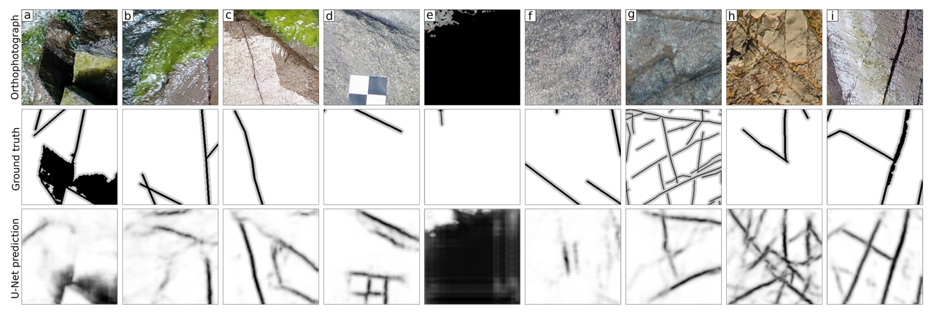
Figure 14 Error case analysis of U-Net predictions. Top row: Orthophotographs (a–c) with water and large shadows, (d) with a black-and-white scale panel, (e) containing missing pixel data, (f) showing no visible fractures, and (g–i) displaying fractures of varying thickness, orientation, and illumination. Middle row: Ground-truth annotations. Some overrepresent shadows due to preprocessing (a), contain labelling errors (c), have over-simplified traces (h), or show omissions (i). Bottom row: U-Net probability maps. Spurious responses appear in (a–e) due to input artifacts or preprocessing issues, while the model captures more realistic fracture geometry than the annotations in (f–i).

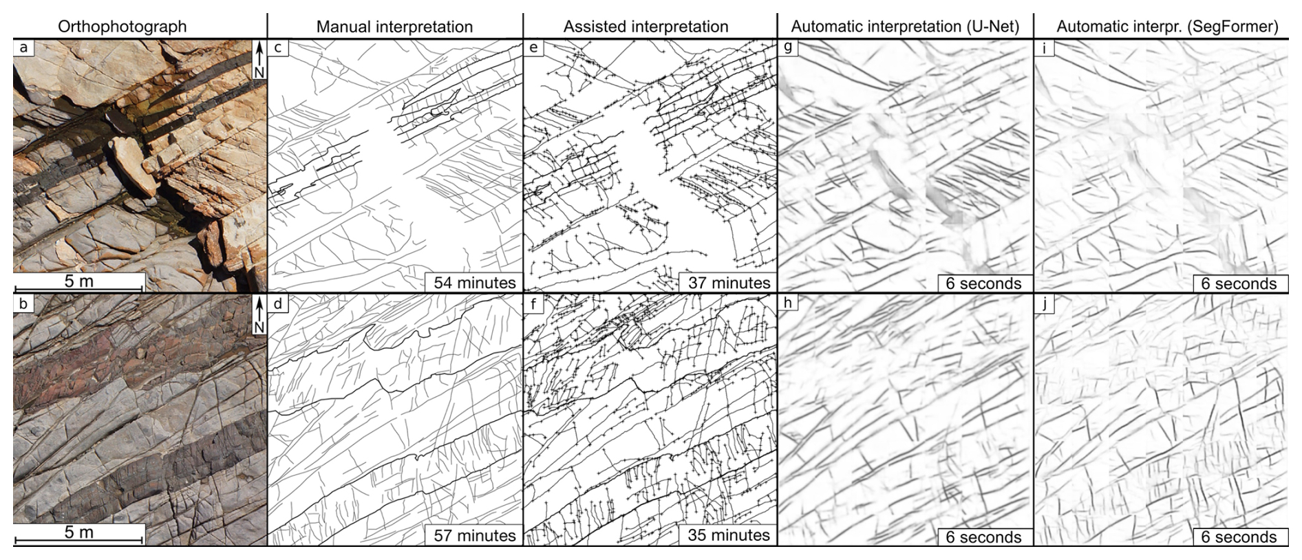
Figure 15 Two 10 m × 10 m orthophotographs (Thiele et al., 2017b, a) (a, b) with corresponding fracture traces digitised manually (Thiele et al., 2017b) (c, d), semi-automatically using the assisted method of (Thiele et al., 2017b) (e, f), automatically with the U-Net model (g, h) and with SegFormer model (i, j).

3.2.5 Error Case Analysis

Despite its stronger overall performance, the U-Net still produced errors (Fig. 14). These fall into two categories: (1) cases where the model was highly confident yet disagreed with the annotations, and (2) cases where the model was uncertain, assigning low probabilities and yielding fragmented or unstable predictions under challenging visual conditions.

High-confidence errors. In several cases, the CNN produced confident predictions that did not match the annotations. A common source was annotation misalignment, where fractures in the ground truth were traced coarsely or offset from the true pixel locations, e.g., the over-simplified traces and omissions visible in Fig. 14h and i. In these cases, the CNN model is arguably more accurate than the ground truth. This misalignment was particularly evident in the Samsu19 dataset, where manual traces did not precisely follow pixel-level fracture geometry.

Another high-confidence error type was input data artifacts, especially in Matteo21, where corrupted pixel values (NaNs, which PyTorch converts to 0, rendering them black in RGB) in the RGB channels led to localised false positives or spurious losses unrelated to actual geological structures, as illustrated by the missing pixel data in Fig. 14e and the resulting spurious responses in the corresponding probability map.

Low-confidence errors. Other errors occurred when the model was less certain and produced scattered or incomplete predictions. Confounding visual features such as vegetation, weathering textures, or shadows were occasionally misclassified as fractures, but with lower confidence values in the probability maps – as seen in the water- and shadow-affected orthophotographs in Fig. 14a–c. Additionally, dataset outliers and preprocessing failures (e.g., unusual lithologies, lighting conditions, mislabelled patches, or the black-and-white scale panel in Fig. 14d) caused the model to generate unstable or inconsistent outputs, while Fig. 14f, which contains no visible fractures, illustrates how the absence of true structure was nonetheless handled by the model. These low-confidence cases reflected the difficulty of generalising across heterogeneous field conditions not fully represented in the training data.

Taken together, this analysis suggests that many errors stemmed not from the CNN architecture itself but from data limitations: annotation quality, input artifacts, and domain heterogeneity. Probability maps proved useful here: they allowed us to distinguish between errors where the model was confident but the labels were unreliable, and those where the model itself was uncertain – as summarised across the panels of Fig. 14, including the varying fracture thickness, orientation, and illumination shown in Fig. 14g–i.

3.2.6 Time Required

We compared the time required for fracture mapping across manual, assisted, and automatic approaches (Fig. 15). Timing data for manual and assisted interpretation are taken from Thiele et al. (2017b), where mapping fractures in a 10 m × 10 m area at a resolution of 1 cm per pixel took 54–57 min manually and 35–37 min using semi-automatic tools. In contrast, our automatic deep learning approach generated probability maps in 6 s (on a Hugging Face Spaces free-tier instance with 2 vCPUs and 16 GB RAM). While post-processing is still required to derive a fracture map (instance segmentation and vectorisation), this speed-up could substantially reduce the effort and time needed for large-scale fracture interpretation.

4 Discussion

Here we discuss key observations from the benchmarking experiments and their implications for automated fracture mapping.

4.1 Model Performance

Traditional edge and ridge filters proved inadequate for robust fracture mapping across heterogeneous datasets (Figs. 10 and 11, Table E1). Outputs were highly sensitive to parameter choices, and hyperparameters optimal at one site often failed to generalise across combined sites. In practice, traditional methods remain useful for rapid visualisation, exploratory work, or small, tailored datasets, but they are ill-suited for mapping complex fracture systems needed for quantitative fracture and structural analyses.

Our results are consistent with previous U-Net fracture-detection studies. Chudasama et al. (2024) reported F1 scores of 0.78–0.93 on granite outcrops in Finland using U-Net, though their evaluation did not include the background class, which inflates metrics relative to our methodology. Mattéo et al. (2021) achieved a Tversky Index (similar to IoU) of 0.35–0.68 using a similar architecture but on a single lithology. Our M_all model achieves F1 = 0.48 and IoU = 0.31 across heterogeneous datasets with the background class included, suggesting that cross-site generalisation incurs a performance cost that should decrease as more training data become available.

The tested deep learning models outperformed the traditional filters, producing smoother and more continuous traces with substantially better overlap with annotated fractures. Nevertheless, absolute performance remained modest compared with segmentation benchmarks in other domains. This likely reflects the unusual nature of the task – selecting thin (high-aspect-ratio) pixel groupings in a strongly class-imbalanced dataset – and geological and environmental factors that alter fracture appearance or introduce confounding features. Label noise and misalignment are also likely contributors, although practical limits on data collection and manual labelling make better training data hard to acquire.

The transformer-based model (SegFormer) behaved differently from the CNN in our experiments (see Sect. 3.2 and Fig. 13). SegFormer's results were less robust, with spurious detections that we attribute to global-attention mechanisms over-interpreting background structure when the training signal is weak. This is consistent with known properties of transformers: they can excel when supplied with large, diverse, and clean datasets, but are more data-hungry than convolutional architectures.

Transformers showed some promise, but their advantages likely emerge only with substantially larger and cleaner datasets – difficult given practical limits on collecting and labelling geological fracture data. For current data scales, U-Net remains the recommended architecture.

Our cross-dataset experiments show that diverse training data improves performance. A general model trained on all sites consistently outperformed models trained on individual datasets, especially on overlap- and detection-sensitive metrics (F1, IoU). Exposure to varied lithologies, lighting, and fracture patterns appears to yield more transferable features and reduce overfitting to site-specific conditions. These results underscore the value of multi-site datasets for robust fracture segmentation. We caution, however, that lithology- and weathering-specific effects (e.g., grain size, surface staining, or vegetation cover characteristic of a given site) can influence both fracture appearance and model performance; users applying this approach to new settings should validate predictions against site-specific conditions rather than assuming uniform performance across lithologies.

4.2 The Need for Post-processing

A critical bottleneck in automated fracture mapping is post-processing, converting model outputs to polylines or other vectorised fracture instances suitable for topological analyses (e.g., assessing fracture connectivity). Pixel-wise probability maps are valuable, but only a first step toward usable fracture traces. Converting semantic masks into instance-level polylines for length, orientation, and spacing measurements requires robust, standardised post-processing pipelines (skeletonisation, connected-component analysis, cleaning, linking, and polyline extraction). Semantic segmentation models do not explicitly preserve fracture connectivity, so intersections and network topology are often poorly reconstructed even when the main fracture geometries are correctly detected. Without these steps, downstream fracture statistics remain noisy and hard to interpret.

Post-processing should also incorporate domain knowledge (for example, weak orientation priors) to reduce spurious short segments and improve the geological plausibility of extracted traces. Furthermore, post-processing algorithms could leverage the rich information in probabilistic model outputs and local knowledge (e.g., likely fracture orientations) to (1) identify and remove false-positive fracture detections, and (2) extrapolate detected fractures across small gaps based on their orientation, as is commonly done by human interpreters.

4.3 Deployment

As a first step toward practical deployment, we developed lightweight interfaces so users can apply the trained models without machine-learning expertise. A web-based application, built with Gradio (Abid et al., 2019) and hosted on Hugging Face Spaces (https://ayoubft-fractex2d-tuto.hf.space, last access: 25 September 2026), enables users to upload paired RGB images and DEMs to obtain deep-learning–based fracture predictions. The interface also provides access to other computer-vision filters and evaluation metrics.

To facilitate integration into existing geological workflows, we additionally developed a simple QGIS plugin (https://plugins.qgis.org/plugins/fraXtex/, last access: 25 September 2026) that enables inference directly within QGIS. Together, these tools show how the proposed workflow can be adopted in geoscience workflows.

4.4 Implications for Fracture Network Analysis

Beyond raw segmentation accuracy, the speed of the automated workflow has direct implications for fracture network analysis. Our timing comparison (Sect. 3.2.6) shows that generating a fracture probability map takes seconds rather than the tens of minutes to hours required for manual or semi-automated interpretation of an equivalent area (Thiele et al., 2017b). This speed-up changes what is practically feasible: instead of interpreter time limiting studies to a handful of representative outcrops, automated mapping makes it tractable to sample fracture networks over larger areas, across more outcrops, or repeatedly through time (e.g., before and after a rockfall or excavation, or across a monitoring interval), producing larger and more statistically robust datasets for connectivity, spacing, and orientation analyses. In academic settings this lowers the barrier to regional-scale fracture network studies that are currently limited by manual digitisation effort, while in industry contexts (e.g., reservoir characterisation, slope stability, or geo-energy site screening) it enables faster turnaround between data acquisition and first-pass structural interpretation. We emphasise that automated segmentation alone does not yet replace the post-processing step needed to obtain topologically consistent fracture networks (Sect. 4.2); rather, it removes the main time bottleneck upstream of that step, making fracture network analysis at scale substantially more accessible.

4.5 Future Work

Our results highlight several concrete next steps toward automated, more objective fracture mapping: improving annotation precision (multi-scale labels, consensus labelling) in training data, expanding dataset diversity by including more sites as additional public data become available, and adopting architectures and loss functions tailored to the unusual thin geometry of fractures. Complementary strategies such as ensembling, transfer learning, and self-supervised pretraining offer promising avenues to improve performance and robustness. Ensembling multiple models can reduce variance and improve prediction stability, particularly for thin and discontinuous fracture traces. Transfer learning from larger geospatial or remote sensing datasets can provide stronger low-level feature representations, enabling better generalisation when labelled fracture data are limited. Self-supervised pretraining on unlabelled imagery can further leverage abundant data to learn domain-specific texture and structure features, improving downstream segmentation accuracy while reducing dependence on extensive manual annotations.

5 Conclusions

We present a harmonised benchmarking framework for fracture mapping in high-resolution outcrop imagery and use it to compare traditional image filters with deep learning methods, including a U-Net convolutional network and a transformer-based model (SegFormer). Our experiments show that deep learning models consistently outperform traditional edge and ridge filters, yielding smoother, more continuous, and qualitatively more plausible traces. This gap shows that algorithmic improvements alone are insufficient: incomplete post-processing, variable label quality, dataset heterogeneity, and the complex information (e.g., topology) needed to identify high-aspect-ratio, typically continuous fractures are the primary barriers to reliable, fully automated fracture extraction. Beyond these empirical results, the principal contributions are the resources we release: the curated datasets, evaluation protocol, and open-source code. We hope these resources will support further work on the challenges outlined above.

Appendix A: Dataset overviews

Overview maps and example tiles for each of the three datasets (Matteo21: Mattéo et al., 2020; Ovaskainen22: Nordbäck and Ovaskainen, 2025; Samsu19: Samsu et al., 2019) are provided in Figs. A1, A2, and A3, complementing the metadata in Table 2. The satellite basemaps in Figs. A1ii, A2b and A3b are Esri World Imagery (Esri, 2026).

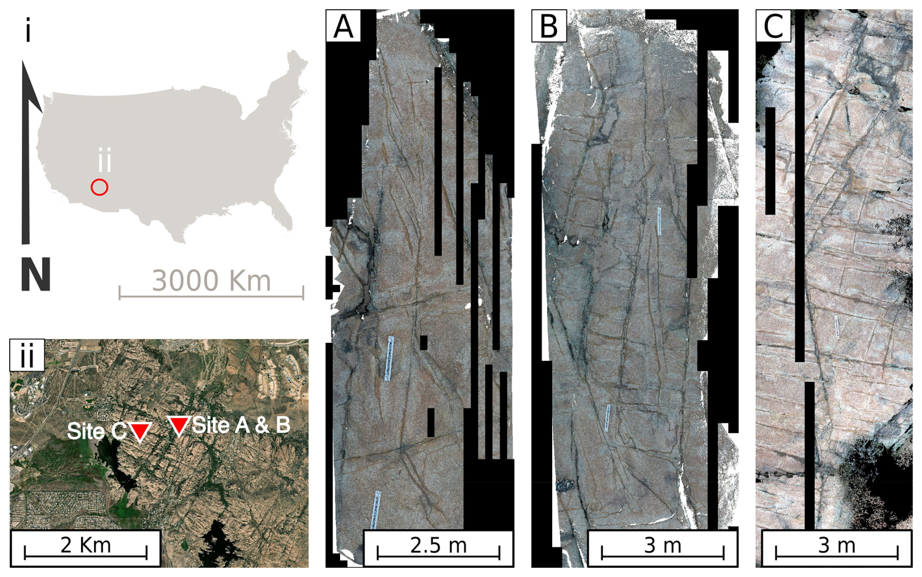
Figure A1 Overview of the Matteo21 dataset (Mattéo et al., 2020). (i) Location map of the Granite Dells, Arizona, USA. (ii) Zoom in to sites A, B and C; basemap: Esri World Imagery (Esri, 2026). (A) Site A (training + validation site). (B) Site B (training + validation site). (C) Site C (test site). Orthophotographs in (A)–(C) from Mattéo et al. (2020).

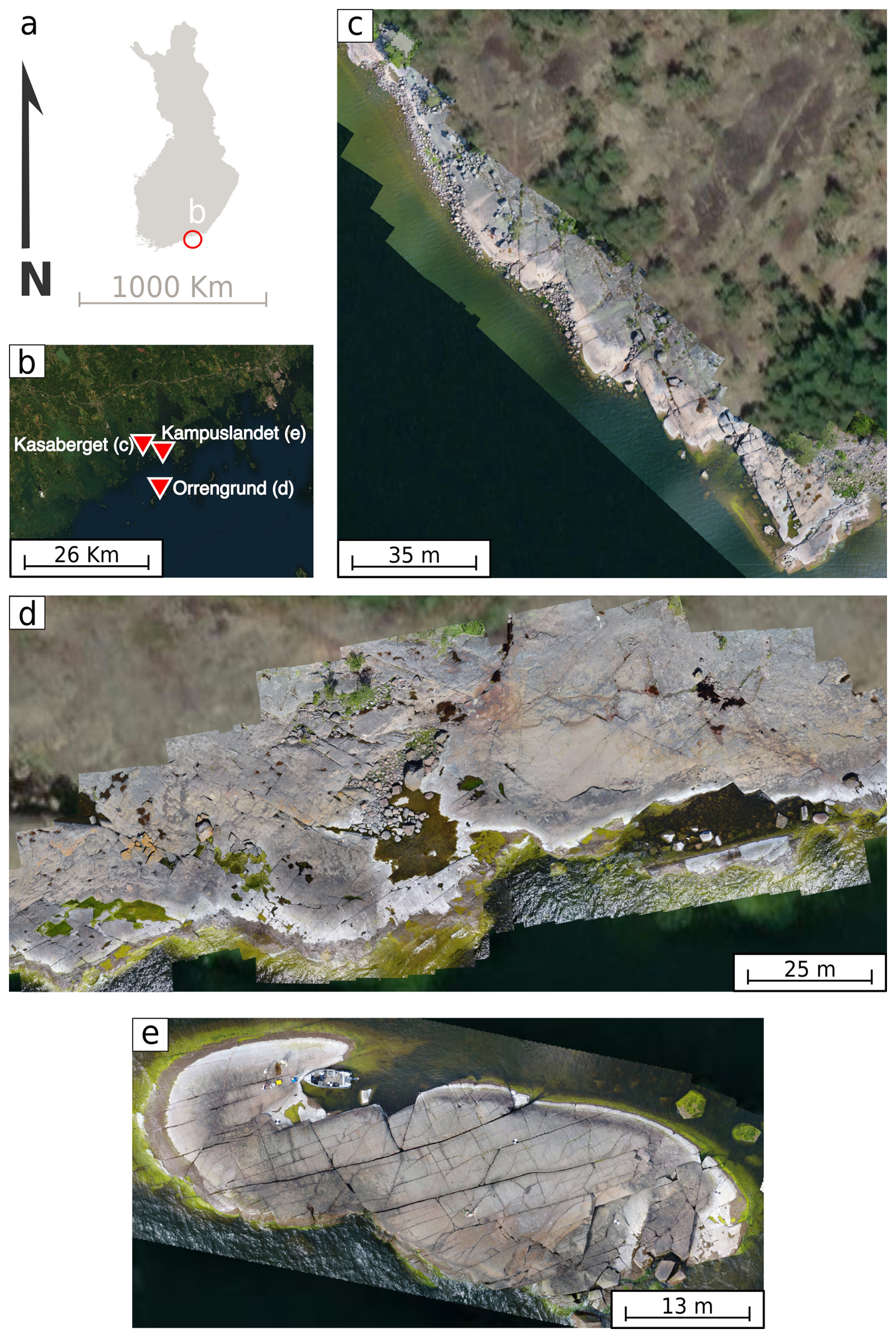
Figure A2 Overview of the Ovaskainen22 dataset (Nordbäck and Ovaskainen, 2025). (a) Location map of the Wiborg Rapakivi Granite Batholith, southeastern Finland. (b) Zoom in to the Loviisa region showing the islands of Orrengrund, Kasaberget, and Kampuslandet; basemap: Esri World Imagery (Esri, 2026). (c) Orrengrund (training site) orthophotograph. (d) Kasaberget (validation site) orthophotograph. (e) Kampuslandet (test site) orthophotograph. Orthophotographs in (c)–(e) from Nordbäck and Ovaskainen (2025).

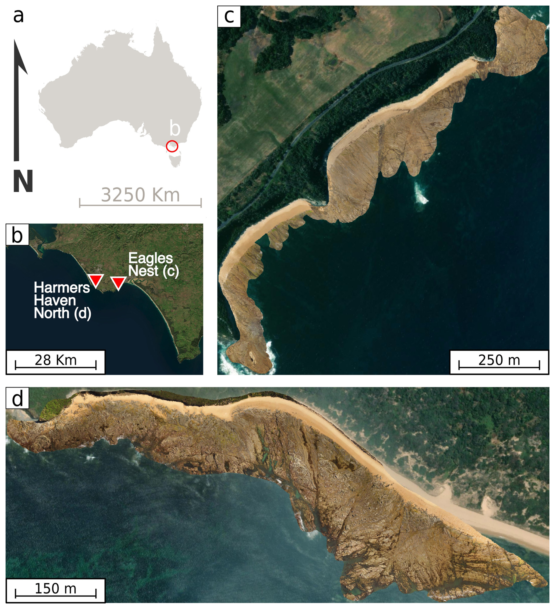
Figure A3 Overview of the Samsu19 dataset (Samsu et al., 2019). (a) Location map of the Strzelecki Group, southeastern Australia. (b) Zoom in to the Harmers Haven area showing Eagles Nest and Harmers Haven North; basemap: Esri World Imagery (Esri, 2026). (c) Eagles Nest (training site) orthophotograph. (d) Harmers Haven North (validation/test site) orthophotograph. Orthophotographs in (c) and (d) from Samsu et al. (2019).

Appendix B: Pre-processing effect

Table B1 Effect of preprocessing on fracture-class pixel proportions across datasets.

Appendix C: Data Augmentation Setup

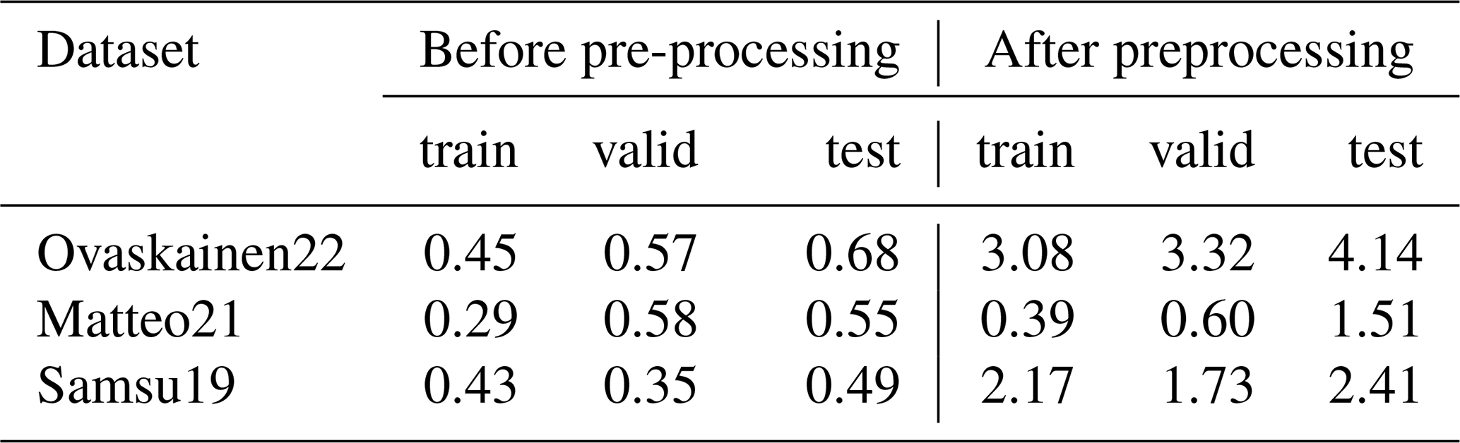
Table C1 Data augmentation techniques and corresponding probabilities and parameter ranges.

Appendix D: Optimal Filters' Parameters

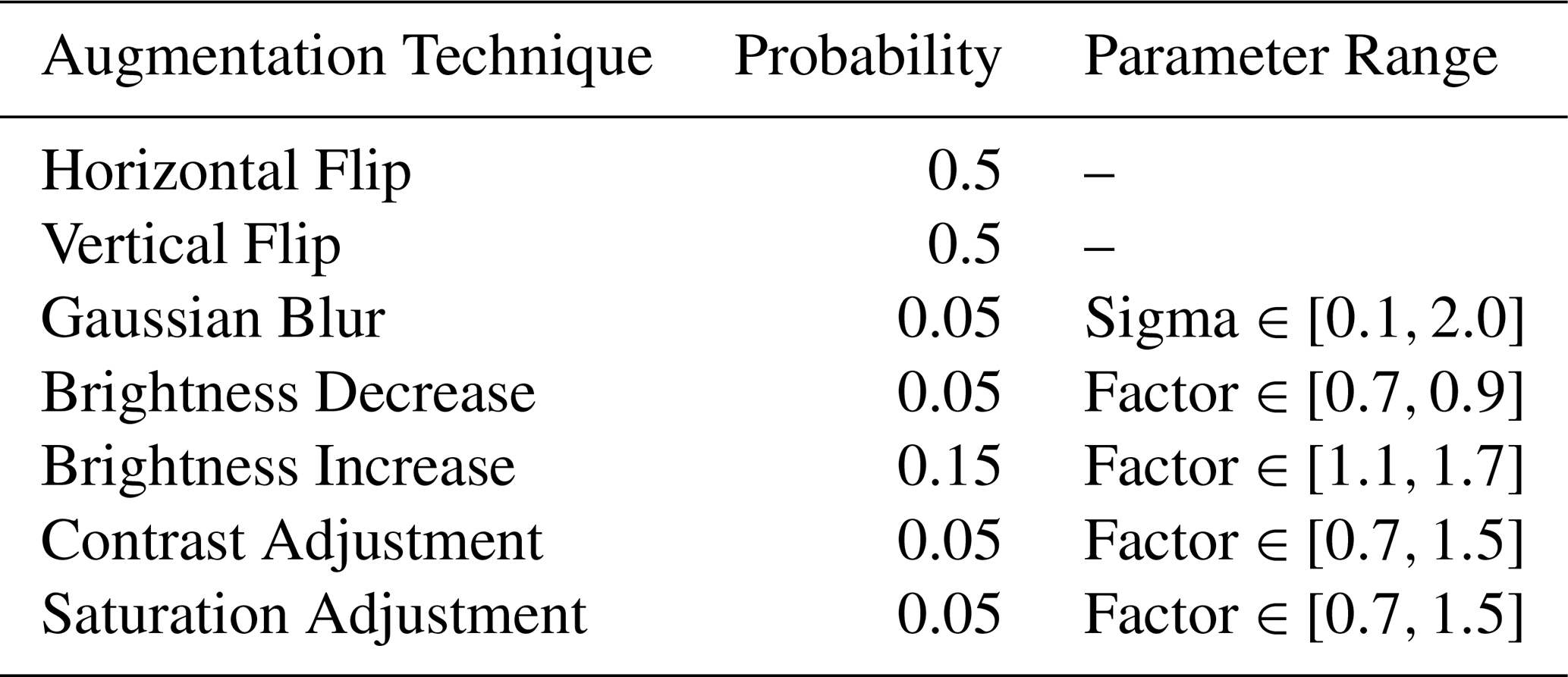
Table D1 Optimal filters' parameters using the grid search and visually (Ovaskainen22/Matteo21/Samsu19/LapiesdiBou).

Appendix E: Quantitative Results

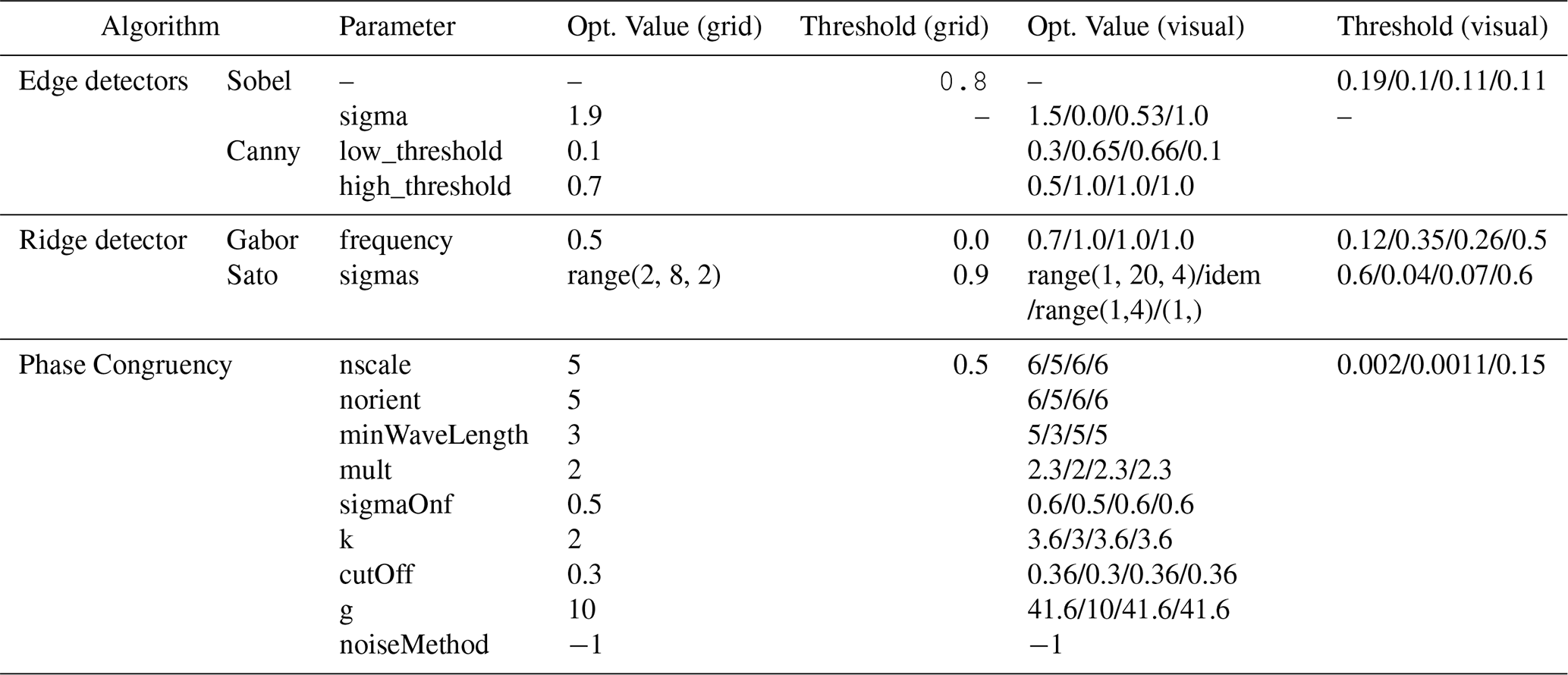
Table E1 Quantitative results: evaluation metrics on the test set. For each metric, the best value is shown in bold and the second-best value in italics.

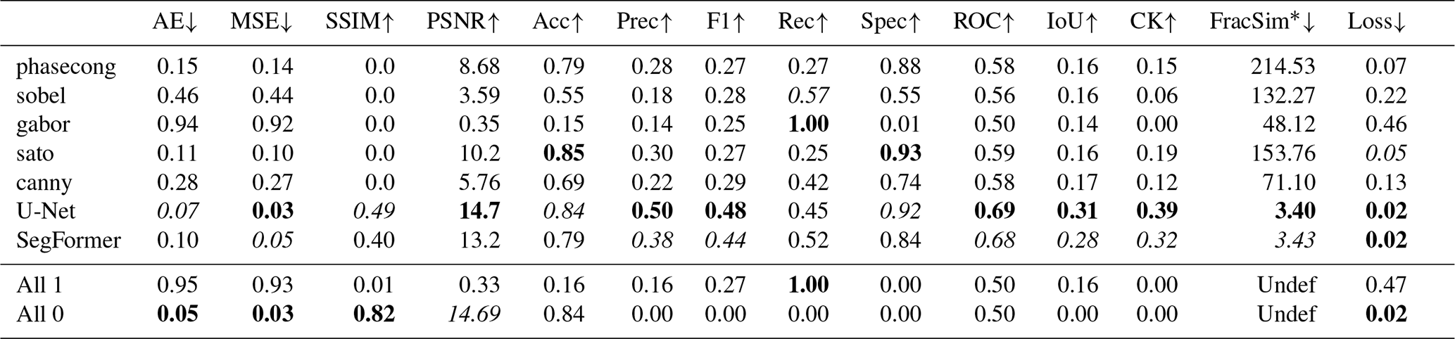
^∗ was calculated on the modified test set