Efficient Uzawa algorithms with projection strategies for geodynamic Stokes flow

Stokes equations are often difficult to handle in geodynamic modelling because they form a saddle-point system and involve strong variations in viscosity. In this work, we reformulate the Uzawa iteration through finite element variational principles, replacing the standard algebraic residual with a weighted L² form that yields a robust preconditioned conjugate gradient iteration for the Schur complement system. Residuals are evaluated in weak form, giving an effect similar to that of a mass-matrix preconditioner. We also add a projection step so that the velocity field remains nearly divergence-free. These updates made the solver converge faster and behave more stably than the standard Uzawa method. This reformulation provides a complementary algorithmic perspective on Schur complement preconditioning within the finite element variational framework. The modified approach was tested in several cases, including ABC flow, SolCx, SolKz, mantle convection, block sinking, multisinker, and compressible convection under the Anelastic Liquid Approximation.

1 Introduction

Geodynamic modelling of the mantle and lithosphere is concerned with processes such as subduction (Gerya, 2022; Li and Gurnis, 2023; Sime et al., 2024), continental rifting (Huismans et al., 2001; Brune et al., 2012; So and Yuen, 2015), mantle plume upwelling (Ismail-Zadeh et al., 2006; Negredo et al., 2022; Kim and So, 2020), and lithospheric buckling (Do et al., 2023; Xie et al., 2024). The mantle has a viscosity on the order of 10¹⁹–10²³ Pa s, and the associated flows occur at low Reynolds number. As a result, inertial terms are negligible, and the Navier–Stokes equations reduce to the elliptic Stokes system. This formulation produces large and sparse saddle-point systems that are challenging to solve, especially when viscosity varies by several orders of magnitude and complex rheologies are present (Moresi and Gurnis, 1996; Zhong et al., 2000).

The spatial discretisation of the Stokes equations in geodynamics is frequently performed using finite element (FEM), finite difference (FDM) procedures, or finite volume (FVM) techniques. These algebraic systems retain the saddle-point structure of the velocity–pressure formulation. For this reason, direct solvers are not a realistic method for three-dimensional problems due to memory and computational expense. Due to this reason, iterative Krylov subspace approaches such as the conjugate gradient (CG) method for symmetric positive definite systems (Hestenes and Stiefel, 1952) and the generalized minimal residual method (GMRES) or its flexible variant (FGMRES) for nonsymmetric systems (Saad and Schultz, 1986; Saad, 2003) are often used for large-scale simulations. In the absence of suitable preconditioning, such methods progress slowly, especially when strong viscosity contrasts reduce the conditioning of the operator.

A common strategy is to eliminate the velocity variables and form a reduced Schur complement system for the pressure. The standard Uzawa algorithm (Arrow et al., 1958) applies Richardson-type iterations to this system and recomputes velocity at each step. The method is simple but converges slowly and is sensitive to the relaxation parameter, which limits its use in geodynamic applications. Later studies proposed variants with preconditioning and inexact solves, such as block preconditioners and mass-matrix approximations, to improve efficiency and stability (Cahouet and Chabard, 1988; Elman and Golub, 1994; Chen, 1998; Bai and Wang, 2008). Explicit formulations of adaptive Uzawa and conjugate-directions Uzawa have been presented, showing their relation to gradient and conjugate gradient iterations (Braess, 2001). In geodynamics, Uzawa-type updates have been implemented in mantle convection codes such as CitcomS (Zhong et al., 2000), and scalability studies have evaluated their performance on large parallel systems (Gmeiner et al., 2016). More generally, Schur complement systems can be solved using Krylov methods combined with suitable preconditioners, and much work has focused on block preconditioners, multigrid methods, and algebraic strategies for Stokes flow (Silvester and Wathen, 1994; May and Moresi, 2008; Kronbichler et al., 2012), including the weighted BFBT (w-BFBT) preconditioner that incorporates viscosity directly into the Schur complement approximation (Rudi et al., 2017). These approaches are now widely adopted in large-scale mantle convection modelling.

This study revisits the Uzawa framework from a variational perspective. The key observation is that defining residuals through weighted L² inner products in the finite element space recasts the Uzawa iteration as a preconditioned conjugate gradient method for the Schur complement system. Since the entire algorithm is expressed through inner products and variational forms, it naturally leverages the matrix assembly and parallel solver infrastructure available in general-purpose finite element libraries coupled with PETSc. Based on this reformulation, we propose two extensions. The first is a viscosity-weighted residual formulation that serves as a Schur complement preconditioner and whose convergence can be systematically improved. The second is a projection post-processing step that improves the divergence-free constraint at minimal additional cost.

The first extension changes how residuals are updated in the pressure space using inner products, which works the same as applying a mass-matrix preconditioner. This connects the L²-projected residual update to preconditioned conjugate gradient (PCG) iterations and brings mass-matrix stabilization into the Uzawa framework (Elman and Golub, 1994; Ramage and Wathen, 1994; Chen, 1998; Benzi et al., 2005). We also introduce a viscosity-weighted variant where the mass matrix is replaced by an η-weighted version. This idea relates to earlier work on Schur complement preconditioners for variable-viscosity Stokes flow (May and Moresi, 2008). Unlike block preconditioning, our method puts viscosity weighting directly into the Uzawa iteration, making it a preconditioned conjugate gradient scheme with a preconditioner that better matches the true Schur complement spectrum. This gives faster and more stable convergence when viscosity contrasts are large.

The second extension is a post-processing projection step that projects velocity variable onto the constraint-satisfying subspace. For incompressible flow, this is the discrete Helmholtz–Hodge decomposition. This method was first introduced for time-dependent Navier-Stokes equations (Chorin, 1967), and later refined for better stability and accuracy (Bell et al., 1989; Guermond and Quartapelle, 1998; Brown et al., 2001; Pyo and Shen, 2007). These methods are standard in unsteady fluid dynamics but have received little attention for elliptic Stokes problems in geodynamics. We use projection after Uzawa iterations to reduce constraint residuals.

The remainder of this paper is organized as follows. Section 2 presents the mathematical formulation, including the Stokes equations, the saddle-point system, Uzawa-type algorithms, residual representations, and the Helmholtz–Hodge projection. Section 3 reports numerical experiments using manufactured benchmarks, incompressible and compressible mantle convection, and block sinking problems. Section 4 summarizes the main results and outlines future work.

2 Mathematical formulation

2.1 Stokes equations and saddle-point formulation

We consider the incompressible Stokes equations relevant to mantle convection. Because the Prandtl number of mantle materials is effectively infinite (Pr ≈ 10²³), inertial terms in the Navier–Stokes equations can be neglected, and the governing system reduces to the elliptic Stokes equations (Schubert et al., 2001).

In a bounded domain Ω ⊂ ${\mathbb{R}}^{n_d}$ (n_d = 2, 3), these are

$$\mathrm{\nabla }\cdot \mathit{\sigma }+\mathit{\rho }\mathbf{g}=\mathbf{0},\mathrm{\nabla }\cdot \mathbf{u}=\mathrm{0},$$

where u is velocity, p is pressure, ρ is density, and g is gravitational acceleration. The Cauchy stress tensor is

$$\mathit{\sigma }=-p\mathbf{I}+\mathrm{2}\mathit{\eta }D\left(\mathbf{u}\right),D\left(\mathbf{u}\right)={\displaystyle \frac{\mathrm{1}}{\mathrm{2}}}\left(\mathrm{\nabla }\mathbf{u}+{\left(\mathrm{\nabla }\mathbf{u}\right)}^T\right),$$

with η the dynamic viscosity and D(u) the strain-rate tensor.

In compact form, the Stokes equations then become

$$\mathrm{\nabla }\cdot \left(\mathit{\eta }\left(\mathrm{\nabla }\mathbf{u}+{\left(\mathrm{\nabla }\mathbf{u}\right)}^T\right)\right)-\mathrm{\nabla }p+\mathit{\rho }\mathbf{g}=\mathbf{0},\mathrm{\nabla }\cdot \mathbf{u}=\mathrm{0}.$$

In the case of constant viscosity with Dirichlet boundary conditions, the momentum equation reduces to a vector Laplacian.

Discretization with stable finite element pairs (Babuška, 1973; Brezzi, 1974; Silvester and Wathen, 1994; Logg et al., 2012) gives the saddle-point system

$$\left(\begin{array}{cc}K& G\\ G^T& \mathrm{0}\end{array}\right)\left(\begin{array}{c}u\\ p\end{array}\right)=\left(\begin{array}{c}f\\ h\end{array}\right),$$

where K is the discrete viscosity matrix (symmetric positive definite) and G is the discrete gradient operator. The system is symmetric but indefinite, and efficient iterative solvers are required.

Eliminating velocity gives the Schur complement system

$$Sp=G^T{K}^{-\mathrm{1}}f-h,S=G^T{K}^{-\mathrm{1}}G.$$

The Schur complement S is symmetric positive definite under the standard inf-sup stability condition. Forming S explicitly is too expensive, since each multiplication requires solving with K⁻¹, which is costly for large problems with variable viscosity. In practice, S is applied implicitly within iterative methods, together with suitable preconditioners.

The standard Uzawa algorithm applies Richardson-type iterations to update the pressure and recompute the velocity, with relaxation parameter ω > 0. The scheme is simple, but its convergence is sensitive to the choice of ω and deteriorates with large viscosity contrasts.

Algorithm 1 Standard Uzawa.

Initialization: Set p⁰=0

Iteration (k≥0):

Velocity update: Find u^k+1 satisfying $K{u}^{k+\mathrm{1}}=f-G{p}^k$

Pressure update: Compute $p^{k+\mathrm{1}}=p^k+\mathit{\omega }(G^T{u}^{k+\mathrm{1}}-h)$

To reduce this sensitivity, the relaxation parameter is updated adaptively at each step. This improves robustness compared with the fixed-ω method.

Algorithm 2 Adaptive Uzawa.

Initialization: Set p⁰=0

Initial solve: Find u¹ satisfying $K{u}^{\mathrm{1}}=f-G{p}^{\mathrm{0}}$

Initial residual: Compute $q^{\mathrm{1}}=h-G^T{u}^{\mathrm{1}}$

Iteration (k≥1):

Auxiliary solve: Find z^k satisfying Kz^k=Gq^k

Step-size selection: Compute ${\mathit{\omega }}_k=(q^k{)}^T{q}^k/(G{q}^k{)}^T{z}^k$

Pressure update: Compute $p^{k+\mathrm{1}}=p^k-{\mathit{\omega }}_k{q}^k$

Velocity update: Compute $u^{k+\mathrm{1}}=u^k+{\mathit{\omega }}_k{z}^k$

Residual update: Compute $q^{k+\mathrm{1}}=h-G^T{u}^{k+\mathrm{1}}$

The CD-U method accelerates convergence by constructing conjugate directions, in analogy with the conjugate gradient method. The explicit coefficients α_k and β_k highlight the connection with CG. By exploiting information from previous steps, CD-U achieves faster and more stable convergence, especially for problems with strong viscosity contrasts or heterogeneous coefficients.

Algorithm 3 Conjugate-Directions Uzawa (CD-U).

Initialization: Set p⁰=0

Initial solve: Find u¹ satisfying $K{u}^{\mathrm{1}}=f-G{p}^{\mathrm{0}}$

Initial residual: Compute $q^{\mathrm{1}}=h-G^T{u}^{\mathrm{1}}$,   set   $d^{\mathrm{1}}=-q^{\mathrm{1}}$

Iteration (k≥1):

Direction solve: Find z^k satisfying Kz^k=Gd^k

Step-size selection: Compute ${\mathit{\alpha }}_k=(q^k{)}^T{q}^k/(G{d}^k{)}^T{z}^k$

Pressure update: Compute $p^{k+\mathrm{1}}=p^k+{\mathit{\alpha }}_k{d}^k$

Velocity update: Compute $u^{k+\mathrm{1}}=u^k-{\mathit{\alpha }}_k{z}^k$

Residual update: Compute $q^{k+\mathrm{1}}=h-G^T{u}^{k+\mathrm{1}}$

Conjugate direction: Compute ${\mathit{\beta }}_k=(q^{k+\mathrm{1}}{)}^T{q}^{k+\mathrm{1}}/(q^k{)}^T{q}^k$,   set   $d^{k+\mathrm{1}}=-q^{k+\mathrm{1}}+{\mathit{\beta }}_k{d}^k$

2.2 Residual representation in Uzawa iterations

The definition of the residual is central to Uzawa-type algorithms. In the Schur complement formulation, the discrete residual is

$$q^k=h-G^T{u}^k,$$

which measures the violation of the incompressibility constraint. In its standard (vector) form, q^k is assembled directly as a discrete vector. This is simple but suffers from poor conditioning, and small singular values of G^T can lead to unstable step-size choices and slow convergence, especially with large viscosity contrasts.

An alternative is to define the residual variationally in the L² inner product on the pressure space Q:

$$\begin{array}{}\text{(1)}& \langle q^k,r\rangle =\langle h+\mathrm{\nabla }\cdot u^k,r\rangle ,\forall r\in Q.\end{array}$$

In discrete form this corresponds to solving a mass-matrix system,

$$M_p{q}^k=M_{p}h+b\left(u^k\right),$$

where b(u^k) denotes the discrete constraint term. This formulation shows that Uzawa iterations implicitly apply the pressure mass matrix as a preconditioner (Cahouet and Chabard, 1988; Elman and Golub, 1994; Chen, 1998; Benzi et al., 2005). The resulting L²-projected residual is smoother and scale-independent, and yields more robust convergence at modest extra cost.

With this modification, the overall update structure of the standard, adaptive, and CD-U algorithms remains the same. Only the scalar coefficients change, as summarized below.

Standard Uzawa.

$$\begin{array}{}\text{(2)}& \langle p^{k+\mathrm{1}},r\rangle =\langle p^k,r\rangle -\mathit{\omega }\langle q^{k+\mathrm{1}},r\rangle ,\forall r\in Q.\end{array}$$

Adaptive Uzawa. Using the L² residual definition in Eq. (1), the step size is updated as

$$\begin{array}{}\text{(3)}& {\mathit{\omega }}_{k+\mathrm{1}}={\displaystyle \frac{\langle q^{k+\mathrm{1}},q^{k+\mathrm{1}}\rangle }{\langle \mathrm{\nabla }{q}^{k+\mathrm{1}},z^{k+\mathrm{1}}\rangle }}.\end{array}$$

Conjugate-directions Uzawa (CD-U). With q^k defined in Eq. (1), the coefficients are

$$\begin{array}{}\text{(4)}& {\mathit{\alpha }}_k={\displaystyle \frac{\langle q^k,q^k\rangle }{\langle \mathrm{\nabla }{d}^k,z^k\rangle }},{\mathit{\beta }}_k={\displaystyle \frac{\langle q^{k+\mathrm{1}},q^{k+\mathrm{1}}\rangle }{\langle q^k,q^k\rangle }}.\end{array}$$

Conjugate-directions Uzawa with η-weighted residuals (CD-U-η). The standard L² residual in Eq. (1) can be extended by replacing the mass matrix with an inverse-viscosity-weighted version, which we refer to as η-weighted for brevity. This introduces a viscosity scaling in the pressure space, which more closely reflects the spectrum of the true Schur complement for variable-viscosity problems. The resulting scheme is a preconditioned conjugate-gradient iteration in which both the residual q^k and its preconditioned form w^k appear in the update formulas.

Algorithm 4 Conjugate-Directions Uzawa with η-weighted residuals (CD-U-η).

Initialization: Set p⁰=0

Initial solve: Find u¹ satisfying $K{u}^{\mathrm{1}}=f-G{p}^{\mathrm{0}}$

Initial residual: Find q¹ satisfying $\langle q^{\mathrm{1}},r\rangle =\langle h+\mathrm{\nabla }\cdot u^{\mathrm{1}},r\rangle$  $\forall r\in Q$

Preconditioning: Find w¹ satisfying $\langle \frac{\mathrm{1}}{\mathit{\eta }}{w}^{\mathrm{1}},r\rangle =\langle q^{\mathrm{1}},r\rangle$   $\forall r\in Q$,   set $d^{\mathrm{1}}=-w^{\mathrm{1}}$

Iteration (k≥1):

Direction solve: Find z^k satisfying Kz^k=Gd^k

Step-size selection: Compute ${\mathit{\alpha }}_k=\langle q^k,w^k\rangle /\langle \mathrm{\nabla }{d}^k,z^k\rangle$

Pressure update: Compute $p^{k+\mathrm{1}}=p^k+{\mathit{\alpha }}_k{d}^k$

Velocity update: Compute $u^{k+\mathrm{1}}=u^k-{\mathit{\alpha }}_k{z}^k$

Residual update: Find q^k+1 satisfying $\langle q^{k+\mathrm{1}},r\rangle =\langle h+\mathrm{\nabla }\cdot u^{k+\mathrm{1}},r\rangle$   $\forall r\in Q$

Preconditioning: Find w^k+1 satisfying $\langle \frac{\mathrm{1}}{\mathit{\eta }}{w}^{k+\mathrm{1}},r\rangle =\langle q^{k+\mathrm{1}},r\rangle$   $\forall r\in Q$

Conjugate direction: Compute ${\mathit{\beta }}_k=\langle q^{k+\mathrm{1}},w^{k+\mathrm{1}}\rangle /\langle q^k,w^k\rangle$,   set   $d^{k+\mathrm{1}}=-w^{k+\mathrm{1}}+{\mathit{\beta }}_k{d}^k$

This iteration can be interpreted as a Preconditioned Conjugate Gradient (PCG) method applied to the Schur complement system. Here q^k denotes the residual in the pressure space, and w^k its preconditioned form. The search directions d^k and coefficients α_k, β_k are then defined from inner products such as 〈q^k,w^k〉, following the standard PCG structure.

With the L² formulation, the preconditioner is the pressure mass matrix M_p, which is spectrally close to the identity. In this case w^k = q^k, and the scheme reduces to a Conjugate Gradient iteration with a trivial preconditioner. In the η-weighted formulation, the preconditioner is the viscosity-weighted mass matrix, so that w^k ≠ q^k and both quantities appear in the iteration. Note that the relation between q^k and w^k cannot be expressed pointwise as w^k=ηq^k, since η(x) varies spatially. Instead, w^k is defined variationally by

$$\langle {\displaystyle \frac{\mathrm{1}}{\mathit{\eta }}}{w}^k,r\rangle =\langle q^k,r\rangle ,\forall r\in Q,$$

which  ensures that w^k  belongs to the pressure space Q  and serves as the Riesz representative of q^k under the η-weighted inner product. This formulation provides a consistent SPD preconditioner in the finite element setting.

In practice, at high resolution or extreme viscosity contrasts, the conjugate gradient iteration may stagnate when the denominators in the step-size and conjugacy coefficients become too small. To address this, we introduce an adaptive scaling parameter AAR that modifies the preconditioner weights from $\mathrm{1}/\mathit{\eta }\left(x\right)$ to AAR $/$ η(x). Starting from AAR = 1.0, the parameter is progressively reduced whenever stagnation is detected. To prevent numerical instability in high-viscosity regions where the scaled weights become excessively small, we enforce a pointwise lower bound ${min}_x(\text{AAR}/\mathit{\eta }(x\left)\right)\ge \mathit{ϵ}$ for a prescribed threshold ϵ. The specific reduction strategy and the threshold ϵ are reported together with the numerical experiments.

In summary, while the L² formulation corresponds to a CG iteration with a trivial mass-matrix preconditioner, the η-weighted Uzawa method is a genuine PCG scheme with a physically motivated preconditioner that better reflects the spectral properties of the Schur complement, particularly under strong viscosity contrasts (May and Moresi, 2008). The adaptive AAR strategy ensures robust convergence of this scheme across a wide range of resolutions and viscosity ratios.

2.3 Helmholtz–Hodge projection as post-processing

Uzawa-type iterations reduce the constraint violation only asymptotically, so the discrete constraint remains slightly violated after a finite number of steps. To enforce the constraint explicitly, we apply a projection step as a post-processing. The idea is to correct an intermediate velocity $\widehat{u}$ by adding a gradient field so that the updated velocity satisfies the discrete constraint operator

$$\mathcal{C}\left(u\right)=h,$$

where 𝒞(u) = ∇⋅u for the incompressible case, and 𝒞(u) = $\mathrm{\nabla }\cdot \left(\stackrel{\mathrm{‾}}{\mathit{\rho }}u\right)$ under the anelastic liquid approximation (ALA).

For the incompressible case, 𝒞(u) = ∇⋅u, the projection requires solving a scalar Poisson problem

$$-\mathrm{\Delta }\mathit{\varphi }=h+\mathrm{\nabla }\cdot \widehat{u},u^{k+\mathrm{1}}=\widehat{u}+\mathrm{\nabla }\mathit{\varphi }.$$

This corresponds to the discrete Helmholtz–Hodge decomposition, which states that any vector field can be uniquely decomposed into a solenoidal part and a gradient part,

$${\mathbf{u}}^{*}=\mathbf{u}+\mathrm{\nabla }\mathit{\varphi },\mathrm{\nabla }\cdot \mathbf{u}=\mathrm{0}.$$

Equivalently, the projection operator can be written as

$$\mathcal{P}=I-G(G^{T}G{)}^{-\mathrm{1}}{G}^T,$$

which is symmetric and idempotent.

In variational form, the correction is obtained by solving

$$\langle \mathrm{\nabla }\mathit{\varphi },\mathrm{\nabla }\mathit{\psi }\rangle =\langle h+\mathrm{\nabla }\cdot \widehat{u},\mathit{\psi }\rangle ,\forall \mathit{\psi }\in Q,$$

and updating the velocity consistently in the finite element space,

$$\langle u^{k+\mathrm{1}},w\rangle =\langle \widehat{u},w\rangle +\langle \mathrm{\nabla }\mathit{\varphi },w\rangle ,\forall w\in V.$$

This weak formulation is important: a direct discrete update u^k+1 = $\widehat{u}$ + Gϕ does not yield the same accuracy, whereas the variational form ensures consistency and better convergence. In practice, the projection can also be implemented component-wise to avoid assembling a large coupled system.

For the compressible case, 𝒞(u) = $\mathrm{\nabla }\cdot \left(\stackrel{\mathrm{‾}}{\mathit{\rho }}u\right)$, and the projection takes the weighted form

$$-\mathrm{\nabla }\cdot \left(\stackrel{\mathrm{‾}}{\mathit{\rho }}\mathrm{\nabla }\mathit{\varphi }\right)=h+\mathrm{\nabla }\cdot \left(\stackrel{\mathrm{‾}}{\mathit{\rho }}\widehat{u}\right),u^{k+\mathrm{1}}=\widehat{u}+\mathrm{\nabla }\mathit{\varphi },$$

so that $\mathrm{\nabla }\cdot \left(\stackrel{\mathrm{‾}}{\mathit{\rho }}{u}^{k+\mathrm{1}}\right)$ = h is satisfied exactly. This weighted projection is the natural extension of the Helmholtz–Hodge decomposition to density-dependent flows.

Although projection methods of this type are standard in computational fluid dynamics, they have not been used previously as post-processing corrections in geodynamics. As we show in Sect. 3, this step reduces accumulated divergence errors and improves the long-term accuracy of mantle convection benchmarks.

A related approach in particle-in-cell methods is the conservative velocity interpolation (CVI) scheme (Wang et al., 2015), which enforces local mass conservation during interpolation but follows a different formulation from the projection-based correction used here. The CVI approach is specifically designed for quadrilateral Q1P0 elements, whereas our projection method is element-independent and applicable to general finite element discretizations.

3 Numerical Implementation

3.1 Finite Element Framework and Parallel Environment

We implemented the proposed algorithms using the open-source finite element library FEniCS (version 2019.2.0.13) (Logg et al., 2012; Alnæs et al., 2015). FEniCS provides a Python interface that simplifies variational form expression and automates finite element matrix assembly, which is useful in geodynamics where PDE systems often involve strongly variable rheologies (Zhamaletdinov et al., 2011; Vynnytska et al., 2013; Wilson et al., 2017; Lee et al., 2024). To solve the large sparse linear systems from discretizing the Stokes equations, we coupled FEniCS with PETSc (Balay et al., 2024). We used GMRES and CG with algebraic multigrid (AMG) preconditioning. Solver configurations were adjusted through PETSc runtime parameters.

All algorithms were implemented within the standard FEniCS–PETSc environment without custom code. This portability shows that the approach is reproducible, extendable, and transferable to other platforms, in line with current practices in large-scale geodynamic modeling.

3.2 Solver configuration and benchmark setup

Each Uzawa iteration with projection requires solving three linear systems: (i) the momentum equation for velocity, (ii) an L²-projection in the pressure space for residual representation and scalar potential projection, and (iii) a Poisson system for velocity correction.

The L²-projection system was solved with CG preconditioned by block Jacobi, which works well for the diagonally dominant mass matrices from finite element discretizations. The Poisson system for velocity correction was also solved with CG and BoomerAMG. All solvers used relative and absolute tolerances of 10⁻¹⁰ and 10⁻¹², so that the convergence behavior observed in our benchmarks is governed by the outer Uzawa iteration rather than by inner solver accuracy. For reference, the ASPECT code (Kronbichler et al., 2012) uses default inner solve tolerances of 10⁻² for the velocity block and 10⁻⁶ for the Schur complement block.

Uzawa iterations were terminated using a normalized divergence residual

$$R_{\mathrm{div}}={\displaystyle \frac{\Vert \mathrm{\nabla }\cdot u^k{\Vert }_{L^{\mathrm{2}}}}{\Vert u^k{\Vert }_{L^{\mathrm{2}}}}},$$

which measures how well the continuity constraint is satisfied. We used relaxed thresholds in long mantle convection runs to balance efficiency and accuracy.

All benchmarks were discretized with Taylor–Hood (P2-P1) finite elements. Geodynamic models often use quadrilateral or hexahedral meshes, but we used structured triangular and tetrahedral meshes generated by splitting each cell along its diagonals. In two dimensions, this diagonal subdivision yields a symmetric “union-jack” pattern that preserves benchmark symmetry. This configuration provides robust velocity-pressure stability and straightforward implementation in FEniCS. Further discussion on finite element selection for geodynamic Stokes modeling can be found in (Thieulot and Bangerth, 2025). Viscosity η is represented as a finite-element field and evaluated at quadrature points during local assembly of element matrices.

To evaluate accuracy, we report the relative L² errors:

$$E_u={\displaystyle \frac{\Vert \mathbf{u}-{\mathbf{u}}_{\mathrm{exact}}{\Vert }_{L^{\mathrm{2}}}}{\Vert {\mathbf{u}}_{\mathrm{exact}}{\Vert }_{L^{\mathrm{2}}}}},E_p={\displaystyle \frac{\Vert p-p_{\mathrm{exact}}{\Vert }_{L^{\mathrm{2}}}}{\Vert p_{\mathrm{exact}}{\Vert }_{L^{\mathrm{2}}}}}.$$

3.3 Baseline comparison of Uzawa variants

We first establish a baseline solver among the three Uzawa variants: standard Uzawa (S-U), adaptive Uzawa (A-U), and conjugate-directions Uzawa (CD-U). For this comparison, we use two complementary tests. The ABC flow with constant viscosity assesses convergence behavior in an ideal setting and is used to compare S-U, A-U, and CD-U directly. The SolCx problem with a viscosity contrast of 10⁶ provides a stress test under strong heterogeneity; here we focus on CD-U and contrast three residual formulations – vector (algebraic), L² inner-product, and the viscosity-weighted CD-U-η – to examine robustness. In both tests, we track the relative L² errors in velocity and pressure and the normalized divergence residual over iterations, and select the most effective configuration for the remainder of the paper.

3.3.1 ABC Flow (smooth analytical solution)

The ABC (Arnold–Beltrami–Childress) flow (Zhao et al., 1993) is used as a smooth manufactured benchmark to compare the three Uzawa variants (S-U, A-U, CD-U) and to select a baseline solver. With constant viscosity (η = 1.0), all residual formulations reduce to the trivial case w^k = q^k. This setting isolates the algorithmic differences among the variants without interference from viscosity contrasts.

The exact velocity and pressure fields are

$$\begin{array}{rl}& \mathbf{u}(x,y,z)=\left(\begin{array}{c}\sin \left(\mathit{\pi }z\right)+\cos \left(\mathit{\pi }y\right)\\ \sin \left(\mathit{\pi }x\right)+\cos \left(\mathit{\pi }z\right)\\ \sin \left(\mathit{\pi }y\right)+\cos \left(\mathit{\pi }x\right)\end{array}\right),\\ & p(x,y,z)=\sin \left(\mathit{\pi }x\right)\cos \left(\mathit{\pi }y\right)\cos \left(\mathit{\pi }z\right).\end{array}$$

Figure 1 shows the relative velocity and pressure errors together with the normalized continuity residual R_div as functions of iteration count. S-U converges very slowly and is highly sensitive to the relaxation parameter. A-U improves robustness but stagnates at higher error levels. CD-U, in contrast, converges rapidly and monotonically for all quantities. These results support choosing CD-U as the baseline solver for the following benchmarks.

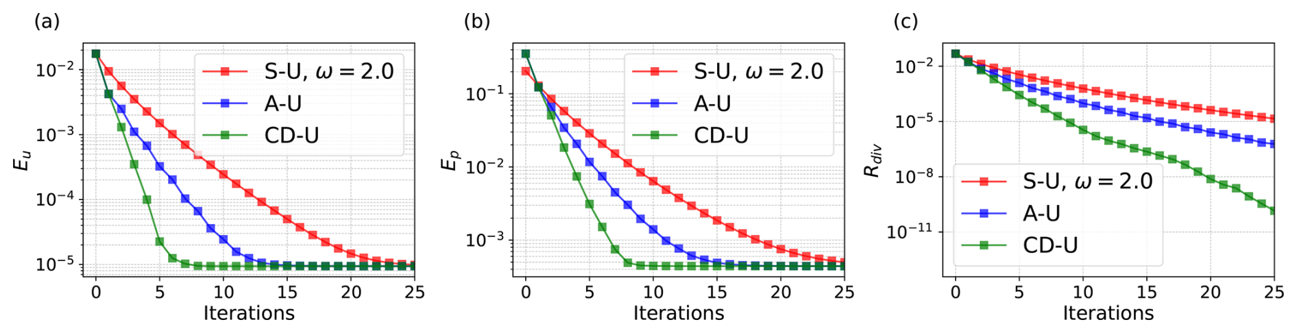
Figure 1 ABC flow benchmark on a 32 × 32 × 32 mesh with P2-P1 elements. (a) Relative velocity error E_u, (b) relative pressure error E_p, and (c) normalized continuity residual R_div as functions of iteration count for the S-U, A-U, and CD-U algorithms.

3.3.2 SolCx (viscosity contrast benchmark)

The SolCx problem (Zhong, 1996) is a standard two-dimensional benchmark for testing solver performance under strong viscosity contrasts. It is posed on Ω = [0,1]² with a discontinuous viscosity,

$$\mathit{\eta }(x,y)=\left\{\begin{array}{ll}\mathrm{1},& x\le \mathrm{0.5},\\ {\mathrm{10}}^{\mathrm{6}},& x>\mathrm{0.5},\end{array}\right.$$

and a density field ρ(x,y) = sin (πy)cos (πx). A gravitational acceleration of unit magnitude ($\left|g\right|$ = 1) was applied in the vertical direction, and reference solutions were taken from Underworld (Mansour et al., 2020; Moresi et al., 2007).

This benchmark poses a challenging test for Uzawa-type solvers. Here we compare three variants of the Conjugate-Directions Uzawa method. The first is the discrete residual update (Algorithm 3), where the residual is updated in purely algebraic (vector) form. The second is the L² inner-product formulation, in which the residual is defined variationally as in Eq. (1), and the update coefficients are computed using the inner-product relations in Eq. (4). Finally, we consider the viscosity-weighted extension CD-U-η (Algorithm 4), which realizes a preconditioned conjugate-gradient method on the Schur complement with a physically motivated η-weighted mass matrix.

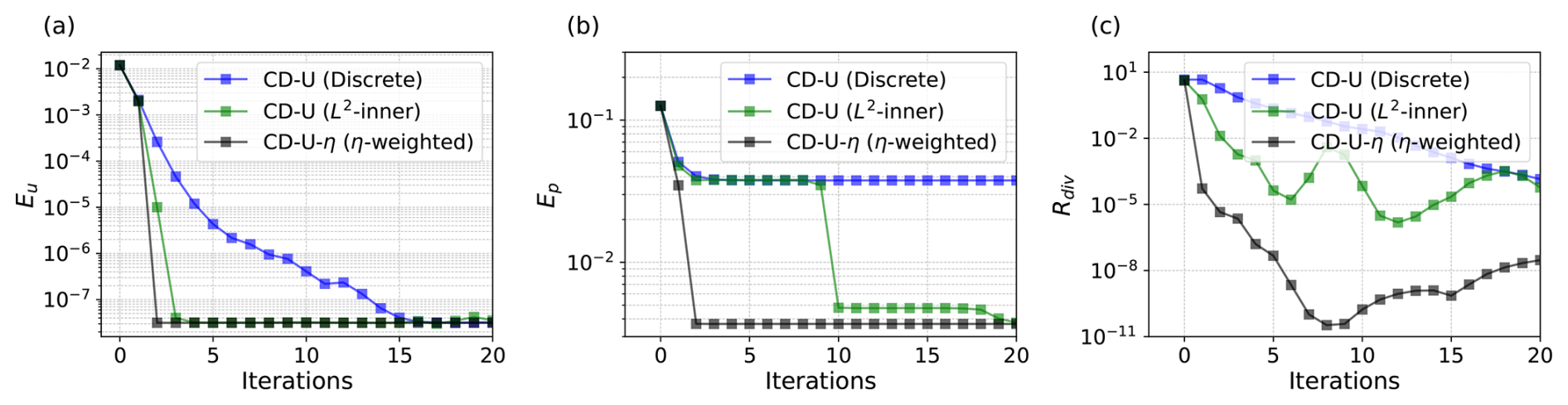
Figure 2 SolCx benchmark with P2-P1 elements. (a) Relative velocity error E_u, (b) relative pressure error E_p, and (c) normalized divergence residual R_div as functions of iteration count for CD-U with discrete update, L² inner-product update, and η-weighted update.

Figure 2 shows that the discrete CD-U update converges slowly and stagnates at high pressure error. The L² inner-product version achieves faster convergence but with oscillations in R_div. The η-weighted variant provides the most rapid initial reduction of velocity and pressure errors and reaches much lower R_div within a few iterations. At later steps, R_div shows a mild increase. This occurs when conjugacy – the orthogonality of successive search directions in the preconditioned Schur complement inner product – degrades due to inexact inner solves for Kz^k = Gd^k and M_ηw^k = q^k. Loss of conjugacy means that a new step partly points back toward earlier directions. Progress measured in the physical L² divergence can be reversed locally, even though the preconditioned CG energy still decreases.

In our numerical experiments, we found that restarts or periodic reinitialization could alleviate this effect. We did not apply them here because the iteration counts are not large enough to require it. Subsequent benchmarks remain stable without reinitialization. The small increase in R_div is a characteristic of the baseline η-weighted formulation rather than a practical limitation.

3.3.3 Multisinker benchmark

The multisinker problem consists of multiple high-viscosity circular inclusions embedded in a low-viscosity medium, driven downward by a gravity-like body force. Unlike the SolCx benchmark with its single planar viscosity discontinuity, the multisinker configuration produces localized viscosity jumps at multiple locations, generating irregular and multiscale flow fields representative of geodynamic settings such as subducting slabs or cratonic roots. We follow the problem setup described in (Rudi et al., 2017).

We consider this problem in two dimensions on the domain Ω = [0,1]² with 8 high-viscosity sinkers centered at prescribed locations c_i, $i=\mathrm{1},\mathrm{\dots },\mathrm{8}$. The viscosity field is defined as

$$\mathit{\eta }\left(\mathbf{x}\right)=\left({\mathit{\eta }}_{max}-{\mathit{\eta }}_{min}\right)\left(\mathrm{1}-{\mathit{\chi }}_{\mathrm{8}}\left(\mathbf{x}\right)\right)+{\mathit{\eta }}_{min},$$

where the indicator function χ₈ accumulates the sinker regions through a product of smoothed Gaussian functions,

$${\mathit{\chi }}_{\mathrm{8}}\left(\mathbf{x}\right)=\prod _{i=\mathrm{1}}^{\mathrm{8}}\left[\mathrm{1}-\exp \left(-\mathit{\delta }max{\left(\mathrm{0},|{\mathbf{c}}_i-\mathbf{x}|-\mathit{\omega }\right)}^{\mathrm{2}}\right)\right],$$

with δ = 200 controlling the sharpness of the viscosity transition and ω = 0.05 the radius of each sinker. Inside the sinkers χ₈≈0 and $\mathit{\eta }\approx {\mathit{\eta }}_{max}$, while in the background χ₈≈1 and $\mathit{\eta }\approx {\mathit{\eta }}_{min}$. The dynamic ratio DR(η) = ${\mathit{\eta }}_{max}/{\mathit{\eta }}_{min}$ was varied from 10² to 10¹⁰, with η_min = DR${}^{-\mathrm{1}/\mathrm{2}}$ and η_max = DR${}^{\mathrm{1}/\mathrm{2}}$. The body force f(x) = $(\mathrm{0},\mathit{\beta }({\mathit{\chi }}_{\mathrm{8}}\left(\mathbf{x}\right)-\mathrm{1}\left)\right)$ with β = 10⁵ acts only inside the sinkers, driving them downward through the lighter, low-viscosity medium. The domain was discretized with 256 × 256 triangular P2-P1 Taylor–Hood elements, and reference solutions were computed using the MUMPS direct solver. Figure 3 shows the viscosity field and the vertical component of the body force for DR(η) = 10¹⁰.

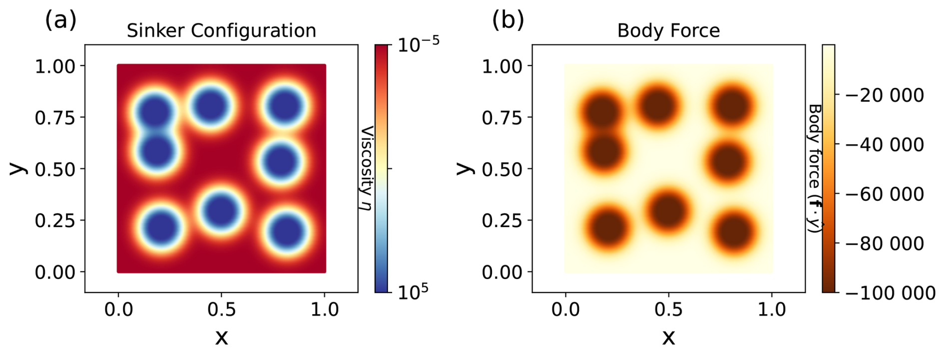
Figure 3 Multisinker benchmark configuration with 8 sinkers and DR(η) = 10¹⁰. (a) Viscosity field and (b) vertical component of the body force.

Since this problem has no analytical solution, convergence was evaluated by measuring relative errors in velocity and pressure against the MUMPS reference solution. Figure 4 shows the convergence history of the CD-U-η solver across dynamic ratios from 10² to 10¹⁰.

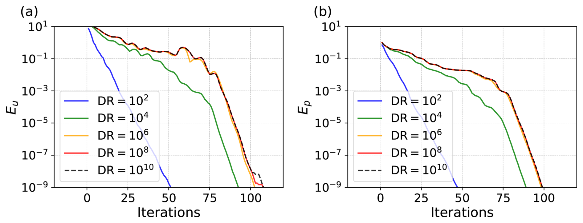
Figure 4 Multisinker benchmark with P2-P1 elements on a 256 × 256 mesh. Convergence of the CD-U-η solver across dynamic ratios from 10² to 10¹⁰. (a) Relative velocity error E_u and (b) relative pressure error E_p as functions of iteration count.

Figure 4 shows that at low dynamic ratios (DR = 10²), the solver converges rapidly. As the dynamic ratio increases, an extended plateau develops in the early iterations before convergence accelerates. This is characteristic of conjugate gradient methods with a poor initial guess. In all experiments, the initial pressure was set to zero, which is far from the true solution for high-viscosity-contrast problems. A better initial pressure estimate could reduce this plateau, but developing such strategies is beyond the scope of this work. For DR ≥ 10⁶, the convergence curves nearly overlap, indicating that the solver becomes insensitive to further increases in viscosity contrast. The pressure error consistently lags behind the velocity error during the initial phase. The adaptive AAR strategy was triggered only for DR = 10⁸ and 10¹⁰ near the final iterations. For this benchmark, stagnation was detected when $|R_{\mathrm{div}}^{k+\mathrm{1}}-R_{\mathrm{div}}^k|<{\mathrm{10}}^{-\mathrm{8}}$ for two consecutive iterations, with a reduction factor of 0.01 and pointwise lower bound ϵ = 10⁻⁸.

3.4 Post-processing strategies for incompressible problems

We next examine the effect of the post-processing correction in two incompressible tests: linear mantle convection with variable viscosity and the block sinking problem with sharp density and viscosity contrasts. In both tests the mesh, boundary conditions, and time stepping are kept identical; the only change is in the Stokes solver. Results from CD-U-η are compared with those from CD-U-η combined with post-processing. Reference solutions are obtained with the direct LU solver MUMPS (Amestoy et al., 2000), which solves the discrete system to near machine precision.

Performance is evaluated by the relative L² errors of velocity and scalar fields (temperature, composition, or density) and by the normalized continuity residual R_div. A breakdown of solver cost is also reported, showing that the post-processing step adds little to the total runtime, while momentum solves remain the dominant cost.

3.4.1 Linear mantle convection

The linear mantle convection benchmark was solved on Ω = [0,2] × [0,1] using a 320 × 160 structured grid, subdivided into triangular P2-P1 Taylor–Hood elements for velocity and pressure. Viscosity followed a depth- and temperature-dependent exponential law (Blankenbach et al., 1989),

$$\begin{array}{rl}& \mathit{\eta }(x,y)=\exp \left(-b{\displaystyle \frac{T}{\mathrm{\Delta }T}}+c(\mathrm{1}-y)\right),b=\log \left(\mathrm{2.5}\right),\\ & c=\log \left(\mathrm{2.0}\right).\end{array}$$

The body force in the Stokes equations was given by thermal and compositional buoyancy,

$$\mathbf{f}=(R{a}_{T}T+R{a}_{\mathit{\varphi }}\mathit{\varphi })\widehat{\mathbf{g}},\widehat{\mathbf{g}}=(\mathrm{0},-\mathrm{1}),$$

with Rayleigh numbers

$$R{a}_T=R{a}_{\mathit{\varphi }}={\mathrm{10}}^{\mathrm{6}}.$$

Initial temperature was prescribed from boundary-layer theory (van Keken, 1997), and the composition field ϕ was initialized as a dense basal layer (Tan and Gurnis, 2005). Boundary conditions were no-slip at the bottom and free-slip elsewhere for velocity; T = 1 at the bottom and T = 0 at the top with insulating sidewalls; and ϕ = 1 at the bottom with homogeneous Neumann elsewhere. The transport equations for temperature T and composition ϕ are

$${\partial }_{t}T+\mathbf{u}\cdot \mathrm{\nabla }T-\mathrm{\nabla }\cdot \left(\mathit{\kappa }\mathrm{\nabla }T\right)=\mathrm{0},{\partial }_t\mathit{\varphi }+\mathbf{u}\cdot \mathrm{\nabla }\mathit{\varphi }=\mathrm{0},$$

where κ = $k/\left(\mathit{\rho }{c}_p\right)$ denotes the thermal diffusivity, with k the thermal conductivity, ρ the density, and c_p the specific heat capacity. For this benchmark, we set κ = 1. Both fields were discretized with P1 discontinuous Galerkin elements using upwind fluxes. Time integration employed the second-order BDF2 scheme, initialized by backward Euler. The Stokes system was solved at each step with CD-U-η or CD-U-η + Post-processing. Iterations were stopped once the normalized continuity residual R_div fell below 10⁻³.

Figure 5 shows that the post-processing step improves accuracy in all fields. Velocity errors remain smaller at every stage, and the normalized continuity residual R_div is consistently lower. Since the composition and temperature fields are advected by the velocity, they also benefit and show clear error reductions. Over 5000 steps, these corrections accumulate, yielding higher long-term accuracy compared with the baseline solver.

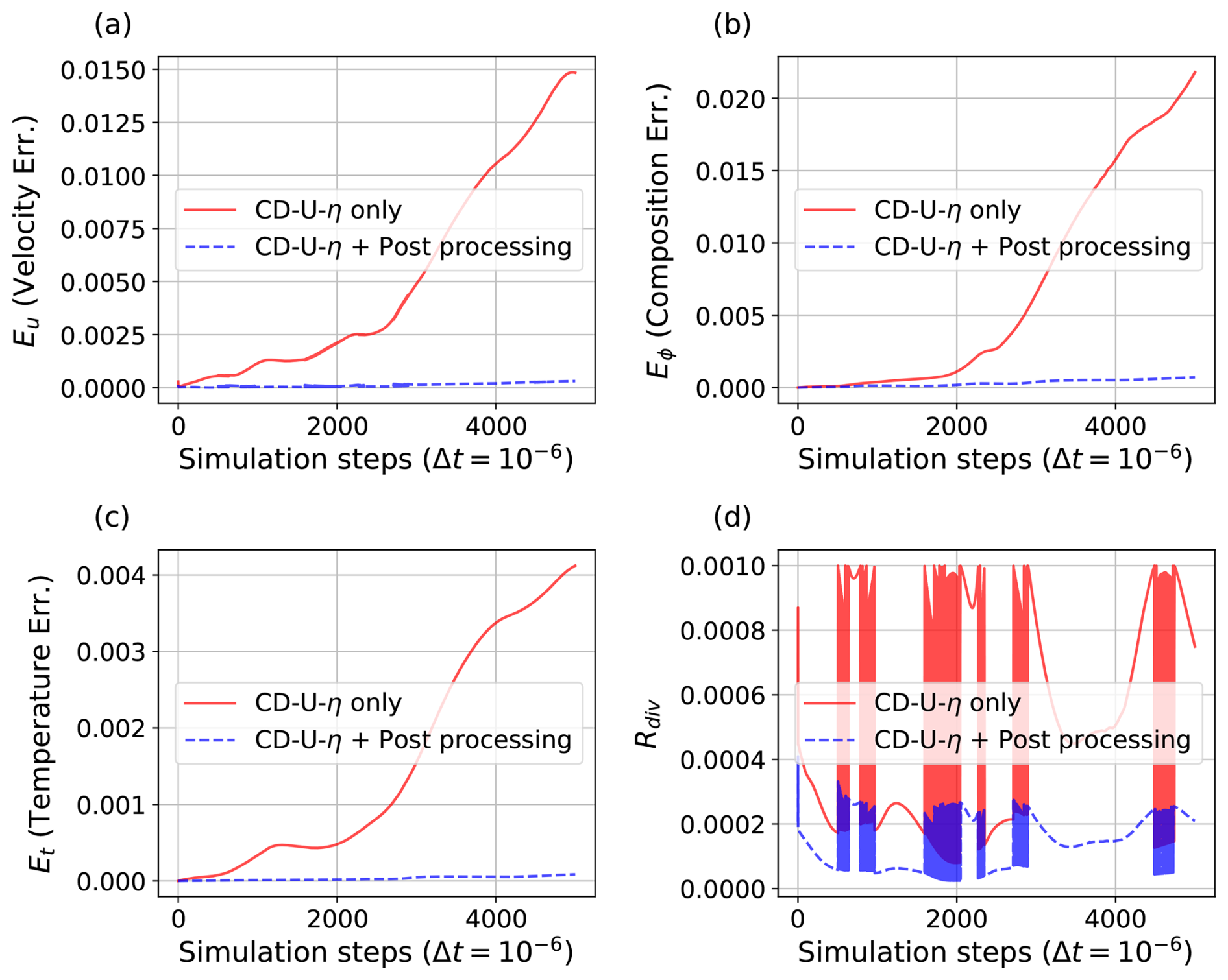
Figure 5 Mantle convection benchmark over 5000 time steps (Δt = 10⁻⁶). Comparison of CD-U-η with and without projection post-processing: (a) relative velocity error, (b) composition error, (c) temperature error, and (d) normalized divergence residual R_div.

Figure 6 shows composition and temperature errors at the final step. CD-U-η alone produces noticeable errors near the interface, especially in the composition field. With post-processing, these localized errors are reduced, and the solution is closer to the reference from the direct LU solver MUMPS, which is effectively exact for the discrete system. This demonstrates that post-processing improves accuracy and aligns the iterative solution more closely with that of a direct solver.

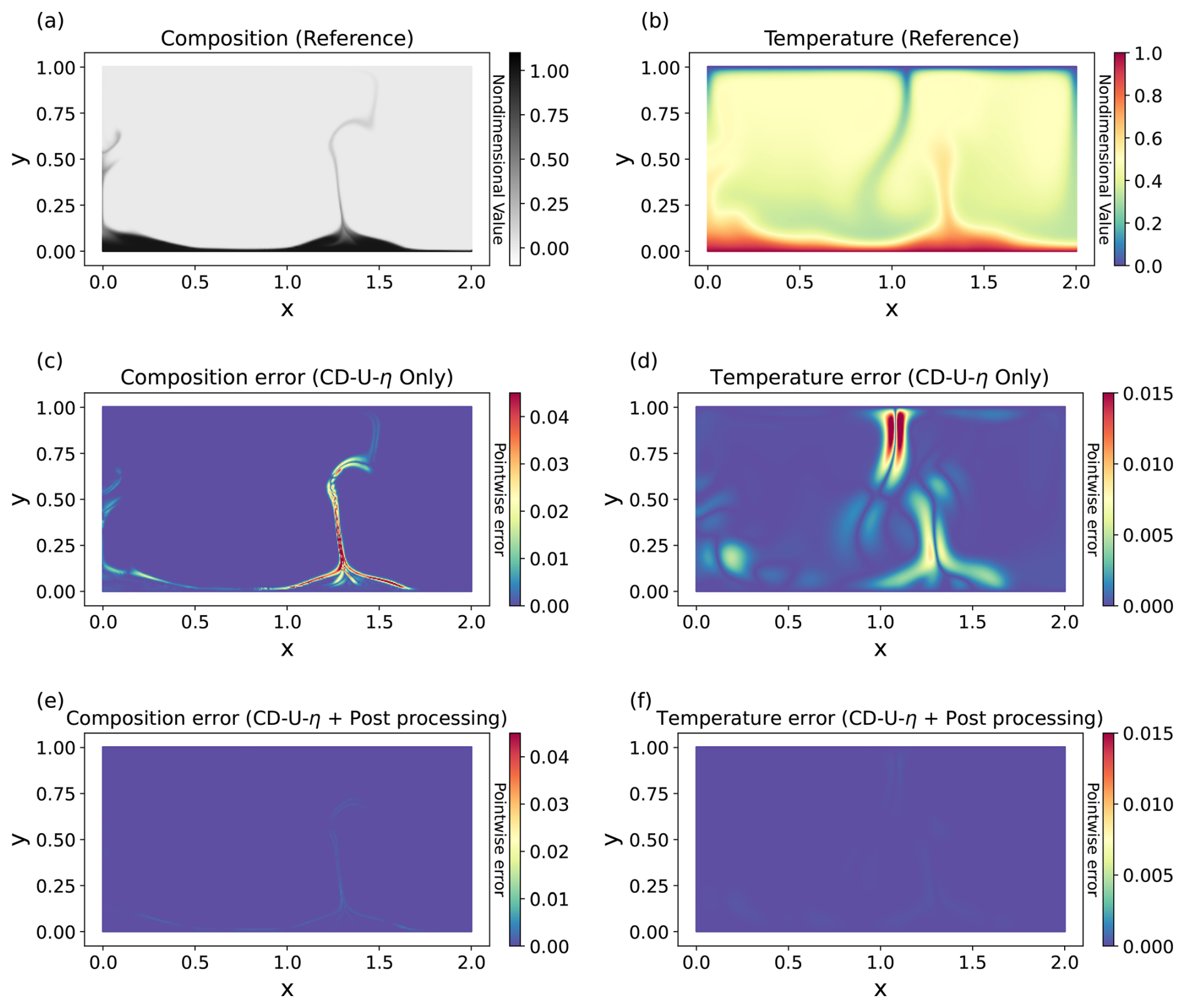
Figure 6 Mantle convection benchmark at time step 5000. Reference fields: (a) composition and (b) temperature. Absolute errors for CD-U-η: (c) composition and (d) temperature. Absolute errors for CD-U-η with projection: (e) composition and (f) temperature.

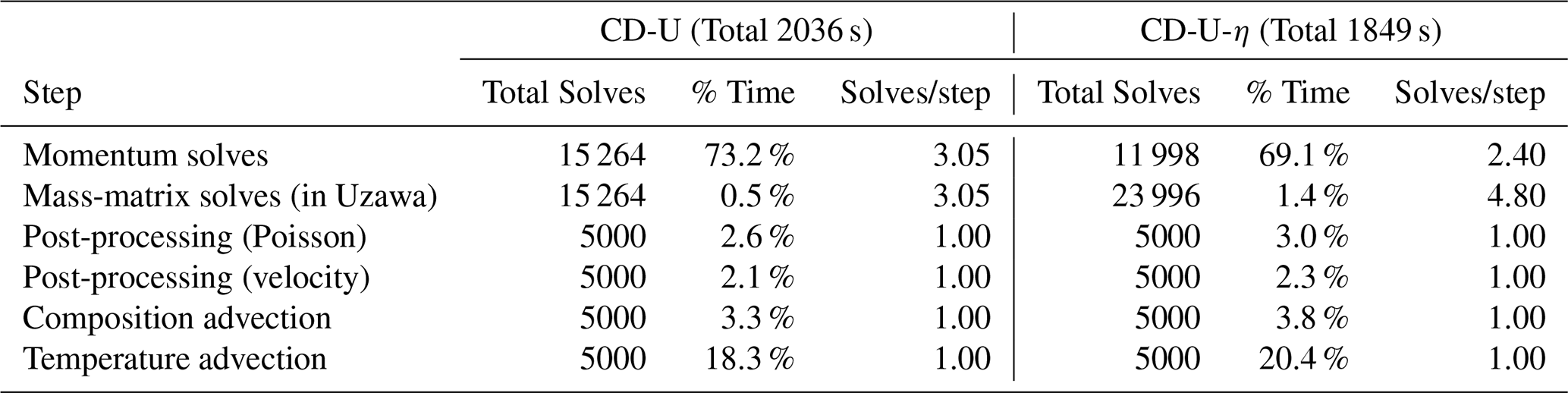
Table 1 summarizes the solver cost for CD-U and CD-U-η with post-processing. The viscosity-weighted variant reduces the average number of momentum solves per step (2.40 vs. 3.05) under the same tolerance, leading to an overall runtime reduction of about 10 %. The extra mass-matrix operations in CD-U-η (two solves per iteration instead of one) are inexpensive, contributing only about 1 %–2 % of the total cost. Similarly, the post-processing corrections, consisting of a Poisson solve and velocity update, account for only a small fraction of the runtime compared with the dominant momentum solves. The main benefit of CD-U-η is therefore the reduction in momentum iterations, while the additional scalar operations have a negligible impact on efficiency.

Table 1 Cost breakdown for 5000 steps (Δt = 10⁻⁶, tolerance 10⁻³, 32 cores). Only solver execution time is included. Both CD-U and CD-U-η are shown with post-processing.

3.4.2 Block sinking problem

The block sinking benchmark (Gerya, 2019) is a two-material Stokes flow test designed to evaluate solver robustness under sharp density and viscosity contrasts. A dense, low-viscosity block sinks into a lighter and more viscous fluid. The interface was represented by a DG0 level-set field (ϕ), positive inside the block, negative outside, and zero on the interface. The level-set was advected in time without reinitialization.

The domain Ω = [0,1]² was discretized with 256 × 256 triangular P2-P1 Taylor–Hood elements for velocity and pressure. The block initially occupied 0.4 ≤ x ≤ 0.6, 0.7 ≤ y ≤ 0.9. Material properties showed strong contrasts: density 4200 vs. 2800, viscosity 0.1 vs. 100. All sides had free-slip boundaries, and the pressure was initialized uniformly. The body force was buoyancy,

$$\mathbf{f}=\mathit{\rho }(x,y)\widehat{\mathbf{g}},\widehat{\mathbf{g}}=(\mathrm{0},-\mathrm{1}),$$

with ρ defined by the block geometry. The level-set was advanced using a Crank–Nicolson scheme.

Solver iterations used a relaxed stopping condition R_div < 0.2 due to the strong viscosity contrasts and interface-driven complexity. This avoided excessive momentum solves under a strict tolerance while still allowing an effective test of the post-processing step. The reference solution was computed with the direct LU solver MUMPS.

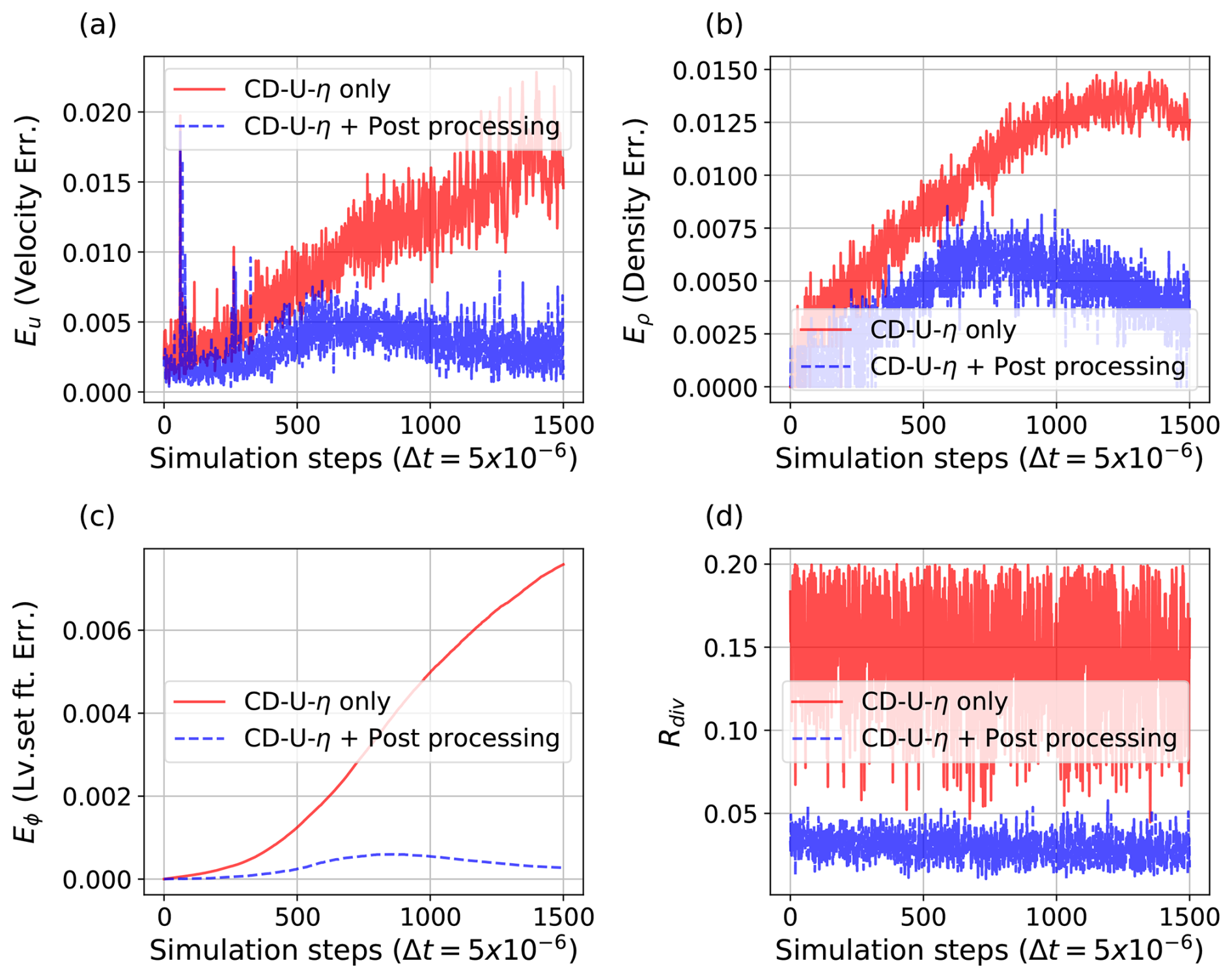
Figure 7 Block sinking benchmark over 1500 time steps (Δt = 5 × 10⁻⁶). Comparison of CD-U-η with and without projection: (a) relative velocity error E_u, (b) density error E_ρ, (c) level-set error E_ϕ, and (d) normalized divergence residual R_div.

Figure 7 shows errors in velocity, density, level-set, and R_div for the block sinking problem. Post-processing decreases both velocity and density errors and suppresses divergence. The irregular pattern in the density error comes from discontinuities along the block interface introduced by the DG0 scheme. The level-set error profile appears smoother. We observed that this reflects the nearly uniform field inside and outside the block. Post-processing helps maintain mass balance and improves agreement with the direct solver.

Figure 8 shows the density and level-set fields at the final step. Large density errors indicate loss of mass conservation, while post-processing reduces these errors and brings the results closer to the reference solution.

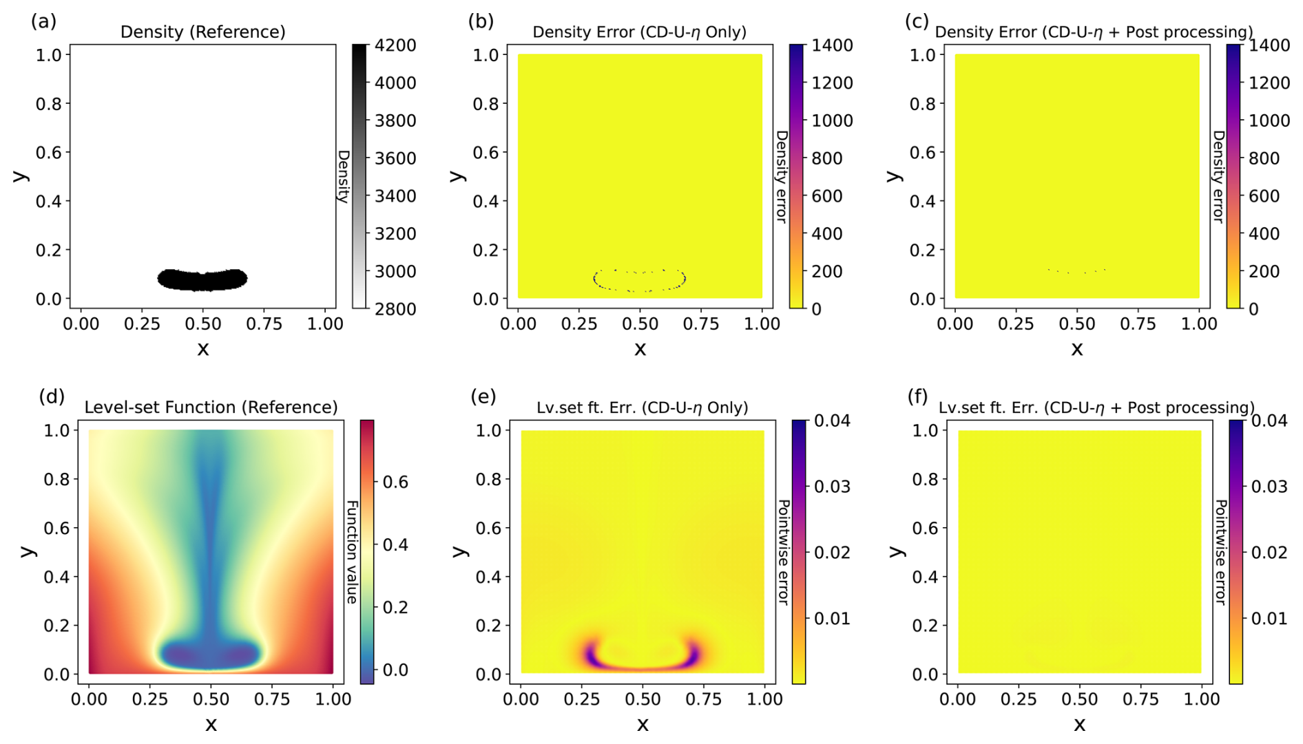
Figure 8 Block sinking benchmark at the final step (1500, Δt = 5 × 10⁻⁶). Density field: (a) reference (MUMPS), (b) CD-U-η, and (c) CD-U-η with projection. Level-set field: (d) reference (MUMPS), (e) CD-U-η, and (f) CD-U-η with projection.

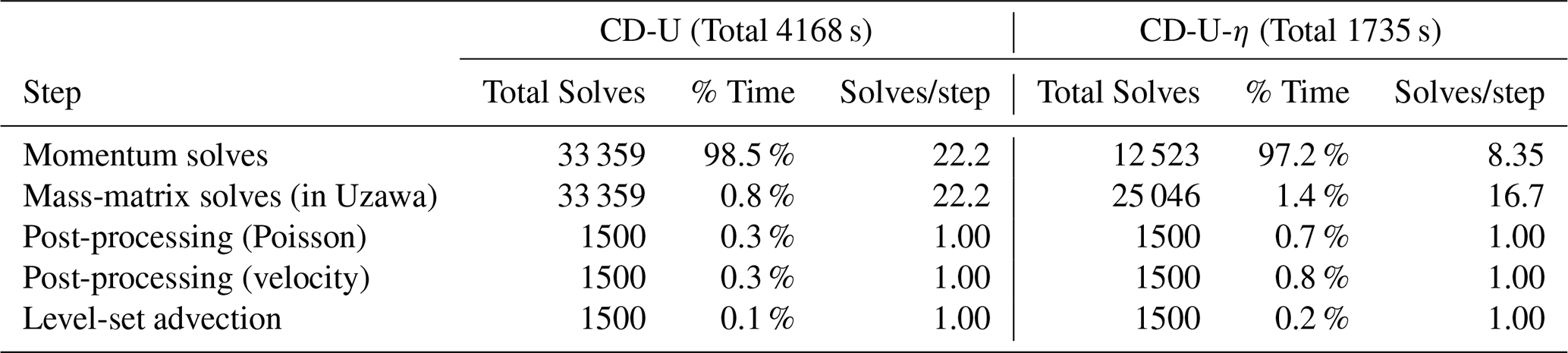
Table 2 compares the solver cost for CD-U and CD-U-η with post-processing in the block sinking problem. The viscosity-weighted variant reduces the average number of momentum solves per step from 22.2 to 8.35, lowering the total runtime from 4168 to 1735 s. The extra mass-matrix solves in CD-U-η are inexpensive, contributing only 1 %–2 % of the total. Post-processing corrections and level-set advection also remain minor. The main benefit of CD-U-η is therefore the smaller iteration count in the momentum equations, while the additional scalar operations add little overhead.

Table 2 Solver cost breakdown for the block sinking simulation (1500 steps, Δt = 5 × 10⁻⁶, tolerance 0.2, 32 cores). Only solver execution time is included.

3.5 Compressible mantle convection

We next consider mantle convection under the Anelastic Liquid Approximation (ALA) (Schubert et al., 2001; King et al., 2008), which incorporates depth-dependent density while filtering out fast acoustic modes. This benchmark follows (King et al., 2008) with Rayleigh number Ra = 10⁵ and dissipation number Di = 0.5. This case extends the projection-based correction to compressible formulations, where mass conservation is weighted by the background density profile.

Under ALA, mass conservation is expressed as

$$\mathrm{\nabla }\cdot \left(\stackrel{\mathrm{‾}}{\mathit{\rho }}\mathbf{u}\right)=\mathrm{0},\stackrel{\mathrm{‾}}{\mathit{\rho }}\left(z\right)={\mathit{\rho }}_{\mathrm{0}}\exp \left({\displaystyle \frac{Di(\mathrm{1}-z)}{{\mathit{\gamma }}_{\mathrm{0}}}}\right).$$

The momentum equation is

$$\mathrm{\nabla }\cdot \mathit{\tau }\left(\mathbf{u}\right)-\mathrm{\nabla }{p}^{\prime }+Ra\stackrel{\mathrm{‾}}{\mathit{\rho }}\mathit{\alpha }T\widehat{\mathbf{k}}-\left({\displaystyle \frac{Di}{{\mathit{\gamma }}_{\mathrm{0}}}}{\displaystyle \frac{c_p}{c_v}}\right)\stackrel{\mathrm{‾}}{\mathit{\rho }}{\mathit{\chi }}_T{p}^{\prime }\widehat{\mathbf{k}}=\mathbf{0},$$

where

$$\mathit{\tau }\left(\mathbf{u}\right)=\mathrm{2}\mathit{\mu }\mathit{\epsilon }\left(\mathbf{u}\right)-{\displaystyle \frac{\mathrm{2}}{\mathrm{3}}}\mathit{\mu }(\mathrm{\nabla }\cdot \mathbf{u})I,\mathit{\epsilon }\left(\mathbf{u}\right)={\displaystyle \frac{\mathrm{1}}{\mathrm{2}}}(\mathrm{\nabla }\mathbf{u}+\mathrm{\nabla }{\mathbf{u}}^{\top }).$$

The temperature equation, including advection, diffusion, adiabatic heating, and viscous dissipation, is

$$\begin{array}{rl}\stackrel{\mathrm{‾}}{\mathit{\rho }}{c}_p{\partial }_{t}T& +\stackrel{\mathrm{‾}}{\mathit{\rho }}{c}_p\mathbf{u}\cdot \mathrm{\nabla }T-\mathrm{\nabla }\cdot \left(\mathit{\kappa }\mathrm{\nabla }\right(\stackrel{\mathrm{‾}}{T}+T\left)\right)+\mathit{\alpha }\stackrel{\mathrm{‾}}{\mathit{\rho }}Di{u}_{y}T\\ & -{\displaystyle \frac{Di}{Ra}}\mathit{\sigma }\left(\mathbf{u}\right):\mathrm{\nabla }\mathbf{u}=\mathrm{0},\end{array}$$

with the background profile

$$\stackrel{\mathrm{‾}}{T}\left(z\right)=T_{\mathrm{0}}\exp \left(Di\right(\mathrm{1}-z\left)\right).$$

Time discretization used a second-order Crank–Nicolson scheme. Since viscosity is constant, CD-U and CD-U-η coincide; the focus here is therefore on testing the robustness of the projection-based correction under compressible mass conservation.

To enforce the weighted continuity constraint after each Uzawa iteration, a $\stackrel{\mathrm{‾}}{\mathit{\rho }}$-weighted velocity correction was applied. Given an intermediate velocity $\widehat{\mathbf{u}}$, we solved

$$-\mathrm{\nabla }\cdot \left(\stackrel{\mathrm{‾}}{\mathit{\rho }}\mathrm{\nabla }\mathit{\varphi }\right)=\mathrm{\nabla }\cdot \left(\stackrel{\mathrm{‾}}{\mathit{\rho }}\widehat{\mathbf{u}}\right),\mathbf{u}=\widehat{\mathbf{u}}+\mathrm{\nabla }\mathit{\varphi },$$

ensuring $\mathrm{\nabla }\cdot \left(\stackrel{\mathrm{‾}}{\mathit{\rho }}\mathbf{u}\right)=\mathrm{0}$ at the discrete level.

The computational domain Ω = [0,1]² was discretized into 160 × 160 triangular Taylor–Hood (P2-P1) elements for velocity and pressure, and P1 discontinuous Galerkin elements for temperature. Viscosity was constant (η = 1). Free-slip boundaries were imposed on the horizontal sides and no-slip on the vertical sides. The temperature was fixed at the bottom (T ≈ 0.09) and top (T = 0), with insulated sidewalls. Initial conditions included sinusoidal perturbations of the background temperature, and pressure was initialized to zero. The Uzawa method with conjugate directions (CD-U) was used as the baseline solver, with convergence tolerance $R_{\mathrm{div}}^{\stackrel{\mathrm{‾}}{\mathit{\rho }}}$ < 10⁻³, and was compared against CD-U with projection-based correction. Reference solutions were computed using the direct solver MUMPS.

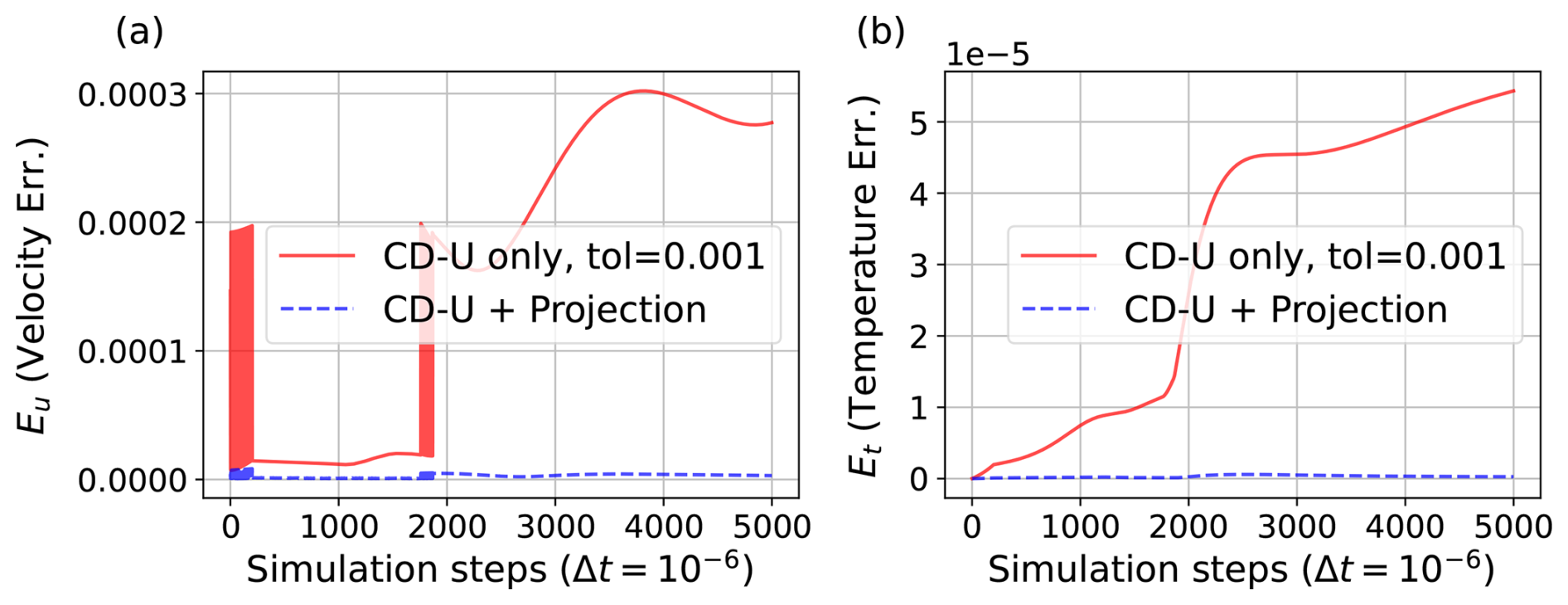
Figure 9 Compressible mantle convection under ALA over 5000 time steps (Δt = 10⁻⁶). (a) Relative velocity error E_u and (b) relative temperature error E_t, comparing CD-U-η with and without $\stackrel{\mathrm{‾}}{\mathit{\rho }}$-weighted velocity correction.

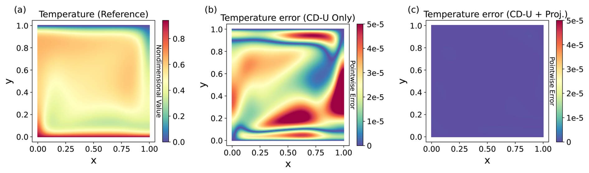
Figure 10 Compressible mantle convection at the final step (5000, Δt = 10⁻⁶). (a) Reference temperature field (MUMPS), (b) absolute temperature error for CD-U-η, and (c) absolute temperature error for CD-U-η with $\stackrel{\mathrm{‾}}{\mathit{\rho }}$-weighted correction.

Figure 9 shows that with constant viscosity the CD-U solver alone is already robust, but the $\stackrel{\mathrm{‾}}{\mathit{\rho }}$-weighted correction further reduces errors in velocity and temperature. Figure 10 confirms improved accuracy near steep thermal gradients.

In terms of cost, the constant-viscosity ALA setup required only about 2–3 momentum solves per step on average, making it considerably cheaper than variable-viscosity cases. The $\stackrel{\mathrm{‾}}{\mathit{\rho }}$-weighted correction added less than 20 % to the runtime, confirming that its accuracy benefits come at modest overhead.

4 Conclusions

We revisited Uzawa-type algorithms for Stokes equations in geodynamics and propose two enhancements. The residual calculation was reformulated in variational form, which provides a natural preconditioner. We then extended this to a viscosity weighting version (CD-U-η). This can be interpreted as a preconditioned conjugate gradient method for the Schur complement. The second enhancement applies a Helmholtz–Hodge projection as post-processing to the velocity field. This enforces the constraint more accurately. Through several benchmark tests, we confirmed that these two approaches help the algorithm obtain more accurate solutions.

Our benchmarks include smooth analytical flows, high-contrast SolCx, SolKz, multisinker, linear mantle convection, block sinking with multiphase interfaces, and compressible mantle convection under ALA. CD-U-η converged faster and stayed robust under large viscosity contrasts. The projection step improved constraint satisfaction and enhanced long-term accuracy. In time-dependent simulations, small corrections at each step accumulated and substantially improved transported fields such as temperature, composition, and density.

In our benchmark tests, the additional cost of L² residual and projection corrections was modest – less than 5 % of total solver time. Momentum solves remained the dominant component. The enhancements do not significantly change the overall cost. As the problem size increases, the relative cost of these corrections should decrease further since momentum solves become more dominant. Additionally, the viscosity-weighted variant helps reduce momentum iterations, further improving computational efficiency.

It is important to note that the projection step only corrects the velocity field and does not directly enhance pressure convergence. This highlights an inherent limitation of projection-based strategies, which are designed to enforce incompressibility. Since pressure plays a critical role in many geodynamic applications, its convergence remains governed by the underlying Uzawa iteration. Our focus here was to improve velocity and advected fields. Improving pressure convergence represents an important direction for future research.

In conclusion, projection-enhanced Uzawa solvers provide an algorithmic perspective on Schur complement preconditioning grounded in finite element variational principles. Since the entire formulation relies on inner products and variational forms, it naturally fits within general-purpose FEM libraries coupled with PETSc, and works across different platforms. The method performs well for both incompressible and compressible mantle convection problems with strong rheological complexity. These findings suggest that projection-enhanced Uzawa solvers can serve as a useful baseline for future work in geodynamic modeling.

Appendix A: Mesh refinement study using the SolKz benchmark

One of the most important properties of a numerical method is its behavior under mesh refinement, which verifies that the discrete solution converges to the continuous solution at the expected rate. All experiments in the main body use a fixed discretization, so we present here a systematic mesh refinement study.

We use the SolKz benchmark (Duretz et al., 2011), a two-dimensional Stokes problem on the unit square Ω = [0,1]² with a smooth, exponentially varying viscosity η(y) = exp (cy) and a dynamic ratio of 10⁶. The body force is chosen so that the analytical solution is known. We chose SolKz over the SolCx benchmark presented in Sect. 3 because the discontinuous viscosity in SolCx reduces solution regularity and prevents observation of optimal convergence rates with P2-P1 Taylor–Hood elements. The domain was discretized with structured triangular meshes from 32 × 32 to 1024 × 1024 using P2-P1 Taylor–Hood elements, and reference solutions were obtained from the Underworld software (Mansour et al., 2020).

Table A1 reports the relative errors and the corresponding convergence orders. The method achieves the optimal convergence rates for P2-P1 Taylor–Hood elements: third order for velocity and second order for pressure. These rates are maintained consistently across all resolutions.

Table A1 Mesh refinement results for the SolKz benchmark using CD-U-η.

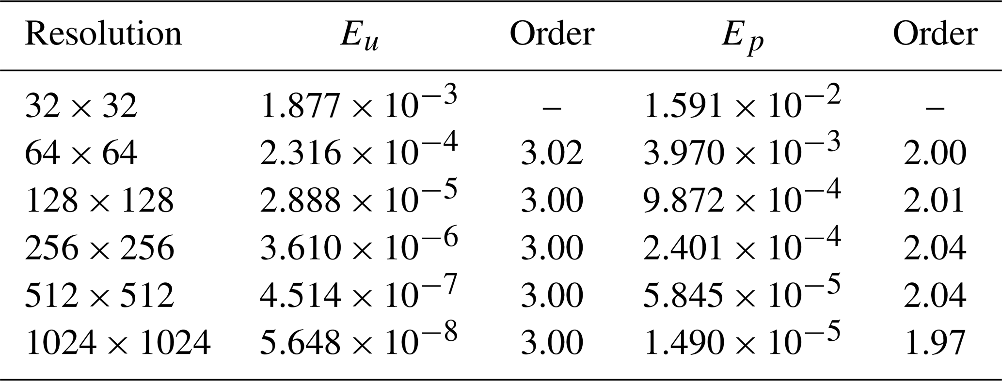
For resolutions up to 256 × 256, the solver converged with AAR = 1.0 without requiring adaptation. At 512 × 512, AAR adjustment occurred occasionally. At 1024 × 1024, the adaptive AAR strategy described in Sect. 2.2 was essential for convergence. For this benchmark, stagnation was detected when $|R_{\mathrm{div}}^{k+\mathrm{1}}-R_{\mathrm{div}}^k|<{\mathrm{10}}^{-\mathrm{10}}$ for two consecutive iterations, and the AAR parameter was reduced by a factor of 0.1 at each trigger. The pointwise lower bound was set to ϵ = 10⁻⁶.

Appendix B: Projection post-processing vs. additional iterations

In time-dependent geodynamic simulations, the Stokes system must be solved at every time step. Iterating to tight convergence tolerances at each step is computationally expensive, since the dominant cost is the momentum solve. In practice, relaxed tolerances are often used to reduce runtime. However, the divergence residual that remains after each solve accumulates over thousands of time steps, degrading the accuracy of advected fields such as temperature, composition, and density. The projection post-processing introduced in Sect. 2.3 offers a potential remedy by enforcing the divergence-free constraint at the cost of only one additional Poisson solve per time step. An alternative strategy is simply to perform additional Uzawa iterations per step. To compare these two approaches in terms of cost and accuracy, we tested both on the mantle convection and block sinking benchmarks from Sect. 3.

In the results below, CD-U-η(niter) denotes n iterations of the CD-U-η solver per time step, and +Proj indicates projection post-processing. Numbers in parentheses show the projection overhead.

Table B1 shows results for the mantle convection benchmark over 5000 steps with Δt = 10⁻⁶.

Table B2 shows results for the block sinking benchmark over 1500 steps with Δt = 5 × 10⁻⁶. For this benchmark, the initial step iterates to tolerance, while subsequent steps use fixed iteration counts with the previous solution as an initial guess.

Table B1 Cost and accuracy comparison for the mantle convection benchmark.

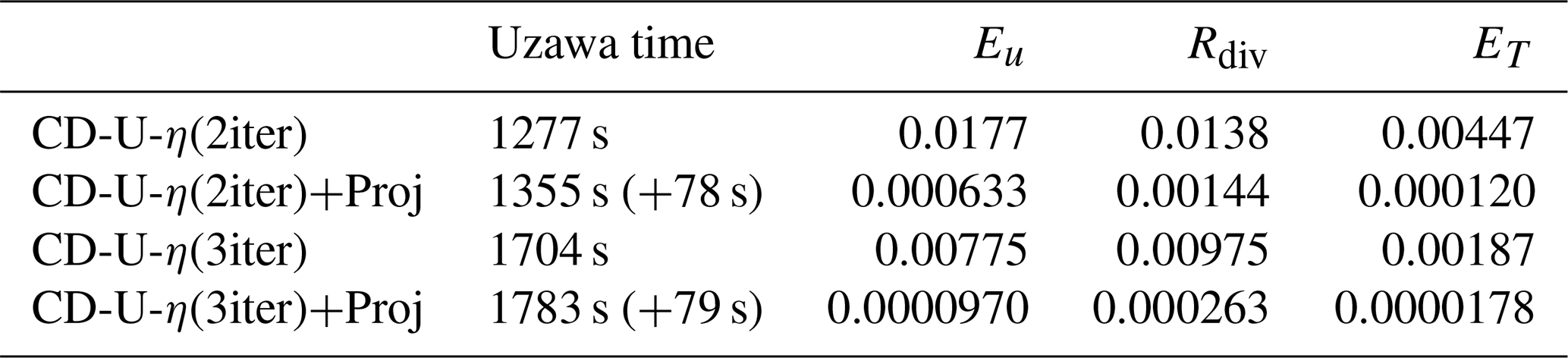
Table B2 Cost and accuracy comparison for the block sinking benchmark.

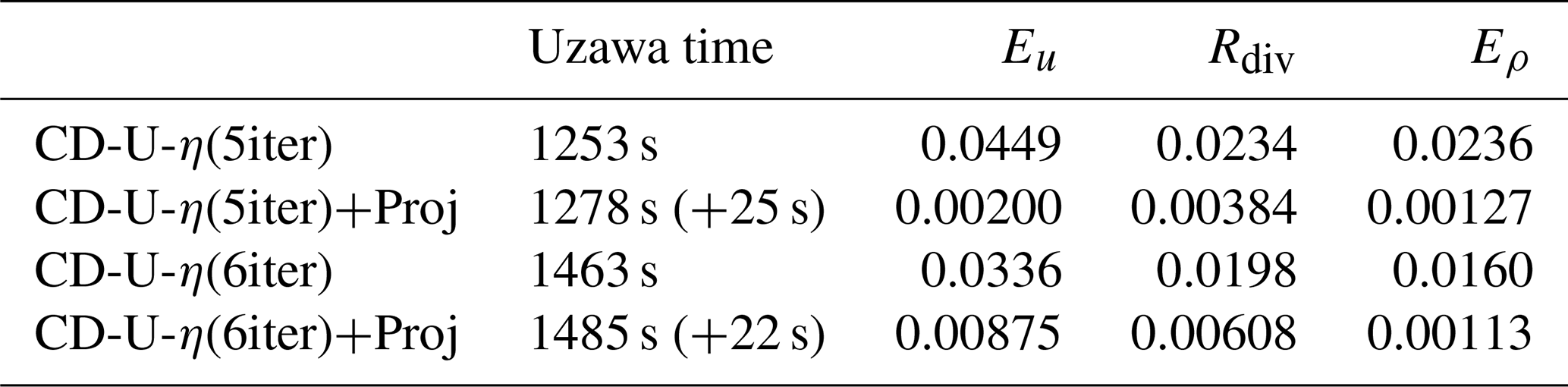
Both benchmarks show that projection adds only a small fraction of the total runtime while substantially improving accuracy. This efficiency comes from the cost difference between the two strategies: each additional Uzawa iteration requires solving the momentum equation, which is the most expensive component, whereas projection requires only one Poisson solve per time step. Moreover, since projection operates as a post-processing step, it is not limited to the Uzawa framework and can be combined with any iterative Stokes solver.

Appendix C: Three-dimensional thermochemical convection

To verify that the CD-U-η algorithm and the projection post-processing operate correctly in three dimensions, we extend the two-dimensional thermochemical convection benchmark of Sect. 3.4.1 by adding a unit-depth lateral dimension. This test also demonstrates the algorithm with Mini elements (P1+Bubble/P1), which satisfy the LBB stability condition independently of the Taylor–Hood elements used in all two-dimensional experiments. Since Mini elements carry fewer degrees of freedom per element than P2-P1 Taylor–Hood elements, they allow finer meshes to be used within the same computational budget, which is particularly advantageous in three dimensions.

The physical setup follows Sect. 3.4.1, extended to the three-dimensional domain [0,2] × [0,1] × [0,1] discretized with a 100 × 50 × 50 structured tetrahedral mesh. Free-slip boundary conditions were applied on the additional sidewalls (y = 0 and y = 1), with insulating conditions for temperature and homogeneous Neumann for composition. All other parameters, including the Rayleigh numbers, viscosity law, initial conditions, and transport discretization, are identical to Sect. 3.4.1. We adopted a fixed time step of Δt = 10⁻⁵, ten times larger than in the two-dimensional case, since the purpose of this test is to verify the algorithmic behavior rather than to assess solution accuracy, and the BDF2 time integration remains stable at this step size. The solution was advanced to the same target time t = 5 × 10⁻³. The Stokes system was solved at each step with CD-U-η, with and without projection post-processing. Iterations were stopped once the normalized continuity residual R_div fell below 10⁻³.

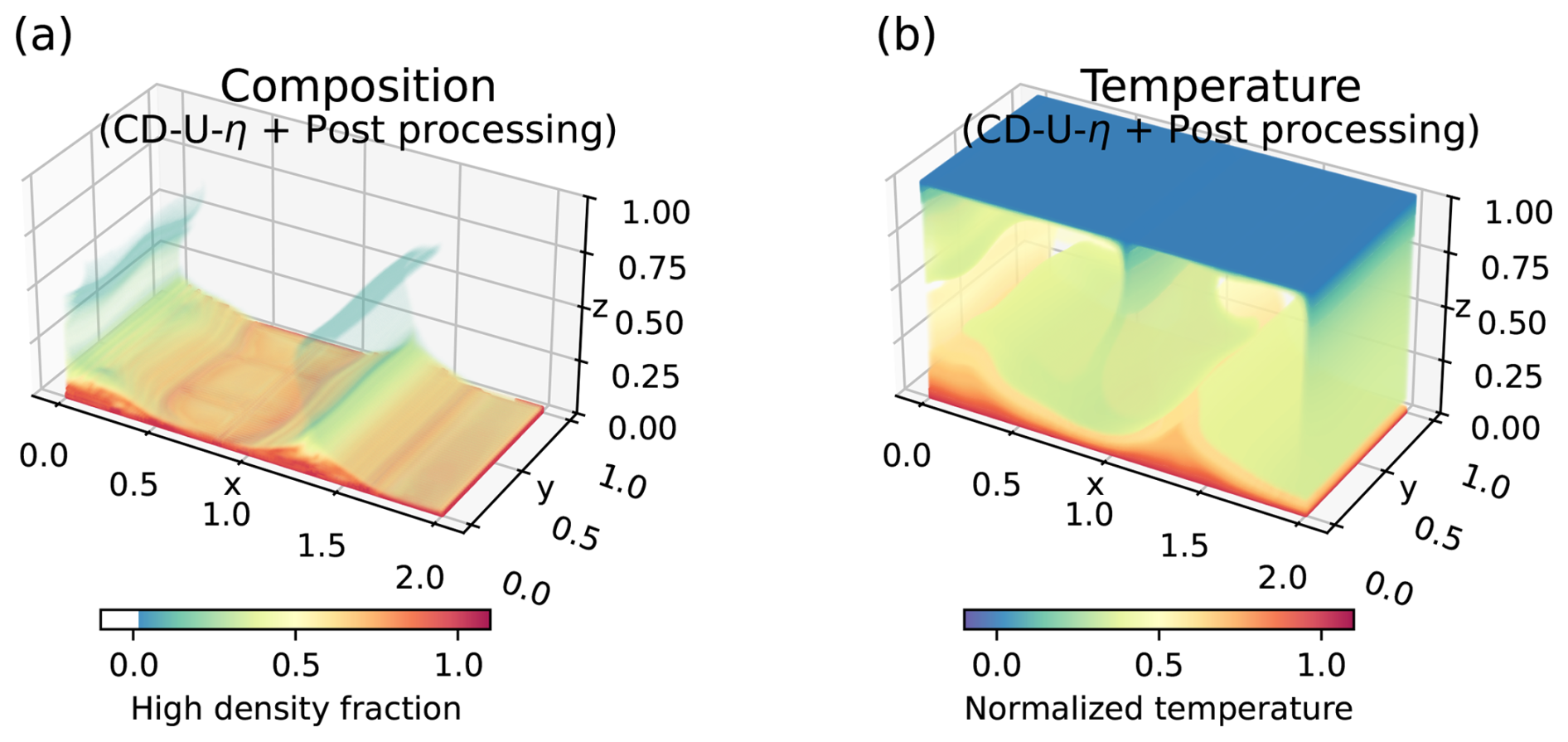
Figure C1 Three-dimensional thermochemical convection at t = 5 × 10⁻³ solved with CD-U-η + projection on a 100 × 50 × 50 Mini element mesh. (a) Composition field showing entrainment of the basal dense layer. (b) Normalized temperature field.

Since a direct solver reference solution is not feasible at this mesh resolution in three dimensions, the comparison focuses on the effect of the projection strategy rather than on accuracy relative to a reference.

Figure C1 shows the composition and temperature fields at t = 5 × 10⁻³, where thermal plumes and entrainment of the basal dense layer are consistent with the two-dimensional results.

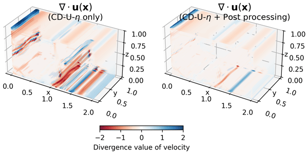
Figure C2a and b show that the projection suppresses the divergence error throughout the domain, with the localized concentrations near the plume regions in (a) largely eliminated in (b). The R_div history in Fig. C2c confirms that this reduction is maintained consistently across all time steps, with the projection lowering R_div by approximately a factor of two, consistent with the two-dimensional results.

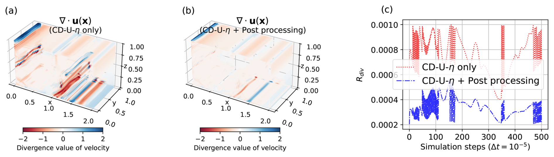
Figure C2 Spatial distribution of ∇⋅u at t = 5 × 10⁻³ for (a) CD-U-η only and (b) CD-U-η + projection. (c) Evolution of the normalized weak divergence residual R_div over 501 time steps for CD-U-η only and CD-U-η + projection.