Spatial influence of fault-related stress perturbations in northern Switzerland

The spatial influence of faults on the crustal stress field is a topic of ongoing debate. While faults are often known to perturb the stress field at a meter scale, their lateral influence over a few hundred meters to several kilometers remains poorly understood. To address this knowledge gap, we use a 3D geomechanical numerical model based on 3D seismic data from northern Switzerland. The model is calibrated with 45 horizontal stress magnitude data obtained from micro-hydraulic fracturing (MHF) and sleeve re-opening (SR) tests conducted in two boreholes in the Zürich Nordost (ZNO) siting region, northern Switzerland. This model with seven faults implemented as contact surfaces serves as the reference model in our study. The reference model is systematically compared to three fault-agnostic models, which share identical rock properties, model dimensions, and calibration data with the reference model, but differ in their element resolution and mechanical properties' assignment procedure. Results show that at distances <1 km from faults, differences in maximum horizontal stress orientation between models range from 3–6°, and horizontal stress magnitude differences are approximately 1–2 MPa. Beyond 1 km, these differences reduce to <1.5° and <0.5 MPa, respectively. These differences are significantly smaller than the calibration data uncertainties at ZNO, which average to ±0.7 MPa and ±3.5 MPa for the minimum horizontal and maximum horizontal stress magnitude, respectively, and ±11° for the maximum horizontal stress orientation. An important implication of our results is that, under the specific geological, mechanical, and stress conditions observed at the ZNO siting region, explicit representation of faults may not be necessary in geomechanical models predicting the stress state of rock volumes located 1 km or more from active faults. This simplification substantially reduced our model setup time from 2 months to 2 days, without compromising the reliability of stress field predictions.

1 Introduction

Characterizing the crustal stress field is essential for understanding both global and local tectonic deformation processes. On a large scale, it provides insights into plate tectonics (Richardson et al., 1979; Cloetingh and Wortel, 1985; Rajabi et al., 2017b) and earthquake mechanics (Sibson, 1992; Sibson et al., 2011; Brodsky et al., 2020), while on a local scale, it plays a critical role in the safe planning of many subsurface applications, including oil and gas exploration and storage (Berard et al., 2008; Zoback, 2009; Fischer and Henk, 2013), geothermal exploration (Catalli et al., 2013; Schoenball et al., 2014; Azzola et al., 2019) and deep geological repositories for nuclear waste (Long and Ewing, 2004; Gens et al., 2009; Jo et al., 2019). The present day stress state also significantly impacts wellbore stability and trajectory optimization, reducing risks and improving drilling operations (Kingsborough et al., 1991; Henk, 2005; Rajabi et al., 2016). Moreover, knowledge of the regional and local stress field aids in assessing seismic hazards and understanding the potential generation or reactivation of faults (Zakharova and Goldberg, 2014; Seithel et al., 2019; Vadacca et al., 2021).

The stress state at a point is described by the Cauchy stress tensor, a symmetric second-order tensor with six independent components. This tensor can be transformed into a principal stress system, where only three mutually perpendicular normal stresses, known as the principal stresses (S₁= maximum principal stress; S₂= intermediate principal stress, and S₃= minimum principal stress), remain, and the shear stresses are zero. In reservoir geomechanics, where the target area is the upper crust, it is typically assumed that the principal stresses are the vertical stress (S_V), the maximum horizontal stress (S_Hmax), and the minimum horizontal stress (S_hmin). Based on this, the reduced stress tensor is defined by the magnitudes of S_V, S_Hmax, and S_hmin, and the orientation of S_Hmax (Jaeger et al., 2007; Zoback, 2009).

The S_Hmax orientation is the most widely available, systematically documented, and freely accessible characteristic of the reduced stress tensor, compiled in a publicly available database of the World Stress Map project (Heidbach et al., 2018; Heidbach et al., 2025a). Analyzing the patterns of the S_Hmax orientation shows consistent trends over hundreds of kilometers in intra-continental areas, primarily driven by first-order plate tectonic forces and second-order buoyancy forces (Zoback et al., 1989; Zoback, 1992; Rajabi et al., 2017b; Heidbach et al., 2018). At the same time, in some regions, significant rotations exceeding 30° are observed on spatial scales ranging from a few tens to a few hundreds of kilometers. It is hypothesized that these variations in S_Hmax orientations, among other reasons, arise from faults (Zoback et al., 1987; Yale, 2003; Heidbach et al., 2007; Tingay et al., 2009; Rajabi et al., 2017b).

A common approach to understanding the fault impact on the stress field is to visually interpret laterally scattered S_Hmax orientation data. This often leads to attributing the observed variability in S_Hmax orientation to the faults present within their respective study areas (Yale et al., 1994; Bell, 1996b; Yale, 2003; Aleksandrowski et al., 1992). While these studies are often convincing, they face two key issues: First, even in areas with relatively high data coverage, such as northern Switzerland (Heidbach et al., 2025a, b) and the northern Bowen Basin (Rajabi et al., 2024; Heidbach et al., 2025a), the data density is fairly low, with, on average, one data record per 138 km² lateral spatial distance, and one data record per 80 km² lateral spatial distance, respectively. Second, individual S_Hmax orientations have an average standard deviation of ±15° (A-Quality) to ±25° (C-Quality), as defined in the World Stress Map (Heidbach et al., 2025a). Together, these issues do not allow for attributing with confidence small rotations in the S_Hmax orientations to the faults, especially at spatial scales of 0.1–10 km.

Notable studies from regions with a comprehensive S_Hmax orientation dataset show that large-scale faulting does not necessarily result in abrupt rotations in the S_Hmax orientation over continental (>500 km) and regional scales (100–500 km). For instance, in eastern Australia, the S_Hmax orientation rotates smoothly, by up to 50° over less than 100 km despite varying dip and strikes of the major fault systems, from northern Bowen Basin to southern Bowen and Surat basins (Brooke-Barnett et al., 2015; Tavener et al., 2017; Rajabi et al., 2024) (Fig. 1a and b). However, in the adjacent Clarence-Moreton Basin, rotation of S_Hmax orientations is prominent and abrupt when viewed in conjunction with the faults (Rajabi et al., 2015, 2017b, c) (Fig. 1a and b). Comparable conflicting trends have been reported in other studies as well (Bell and Gough, 1979; Gough and Bell, 1982; Bell and Grasby, 2012), suggesting that the influence of fault systems on the rotation of S_Hmax orientation at continental and regional scales is not straightforward, and often not resolvable without ambiguity.

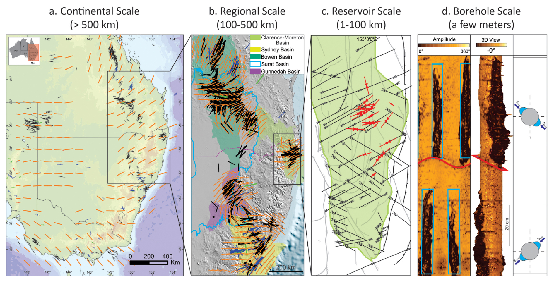
Figure 1 S_Hmax orientation stress map from eastern Australia at (a) Continental scale; (b) Regional scale; (c) Reservoir scale, and (d) Borehole scale. On continental and regional scales, visual observations suggest that faults may have differing influences, as seen in the uniform stress orientation (orange lines) across eastern Australia despite the presence of faults. However, on a borehole scale, faults can cause local perturbations, evident in the shift of borehole breakout orientations (blue box), which reflect stress variations across the fault (red line) (Image adopted from Rajabi et al., 2017c).

At the borehole scale, distinct variations in S_Hmax orientation have been observed vertically on a spatial scale of a few meters. For instance, Fig. 1d shows an image log of a borehole from the Clarence-Moreton Basin, where the S_Hmax orientation abruptly changes by 90° when the borehole intersects a fault. This is also observed in the San Andreas Fault Observatory Drilling Borehole, where borehole breakouts (BO) and drilling-induced tensile fractures (DITF) indicate a change in S_Hmax orientation from 25 ± 10° at 1000–1500 m to 70 ± 14° at 2050–2200 m (Chéry et al., 2004; Hickman and Zoback, 2004; Boness and Zoback, 2006; Zoback et al., 2011). Also, in the KTB drilling program, S_Hmax orientation along the borehole remained consistent with the regional tectonic-induced patterns except at a depth of 7200 m, where a major fault zone caused a localized reorientation by about 60°, confined to only a few meters above and below the fault (Brudy et al., 1993, 1997; Barton and Zoback, 1994).

However, borehole-scale studies are generally conducted in vertical wells and do not capture the potential lateral variations in stress caused by faults. Therefore, it remains unclear whether these localized findings can directly be extrapolated to explain stress field variations at larger spatial scales away from the fault zone. This leads to a significant knowledge gap regarding fault's influence on stress field variations at the reservoir scale (Fig. 1c), a scale particularly important for many subsurface applications. The only viable approach for predicting the variations in the stress field at this scale is geomechanical numerical modelling. Over the past few decades, 2D and 3D geomechanical numerical models have been developed for this purpose (Henk, 2009, 2020; Treffeisen and Henk, 2020). These can broadly be grouped into three categories: (1) site-specific models without fault representation (Lecampion and Lei, 2010; Rajabi et al., 2017c; Ahlers et al., 2021), (2) site-specific models that include faults but are not explicitly focused on assessing influence of faults on the predicted stress (Reiter and Heidbach, 2014; Hergert et al., 2015; Bérard and Desroches, 2021) and (3) generic models that explicitly investigates the impact of faults (Homberg et al., 1997; Su and Stephansson, 1999; Reiter et al., 2024; Ziegler et al., 2024). While models without faults are understandably not suitable for evaluating fault-related stress perturbations, the latter two categories often have limited or no access to reliable in situ stress magnitude data. This hinders their ability to reliably represent fault-related stress variations in real-world scenarios.

In our study, we use 45 reliable and robust stress magnitudes data records, obtained from two deep boreholes, Trüllikon (TRU1-1) and Marthalen (MAR1-1), using microhydraulic fracturing (MHF) and dry sleeve re-opening (SR) test (Desroches et al., 2021a, b, 2023) to calibrate 3D geomechanical numerical models of the Zürich Nordost (ZNO) siting region, northern Switzerland (Fig. 2). The data records were collected during a comprehensive 3D seismic and drilling campaign to support site selection for a deep geological repository (DGR) of radioactive waste (Nagra, 2024c, a). The stress magnitudes presented in this study are the total stresses, and any reference to the stress magnitudes must be taken as such. Four variants of the 3D geomechanical numerical model of the siting region, each with lateral dimensions of 14.7 km×14.8 km, and a vertical depth of 2.5 km below sea level (b.s.l.), are used within this study. All models use identical mechanical properties and the same representation of geomechanically relevant subsurface units. One of the models includes seven contact surfaces with an assigned friction coefficient representing faults, and serves as the reference model (REF model) (Nagra, 2024d, c), while the other three models are fault-agnostic, i.e., faults are excluded from the model. By systematically comparing the predicted stress fields across all the models, we illustrate the observed perturbations in the stress field with respect to the reference model and quantify the spatial extent of the stress perturbations caused by faults.

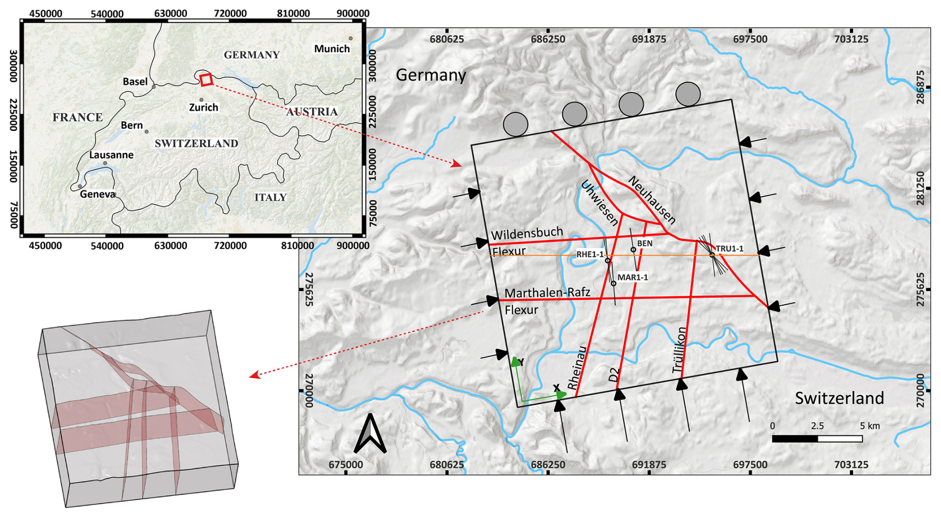
Figure 2 Geographical location and the model boundaries of the ZNO siting region. The red lines within the model extents represent the surface trace of the faults and flexures, interpreted from the seismic sections of the siting region and extrapolated to the surface. The location of the boreholes Trüllikon (TRU1-1), Benken (BEN), Marthalen (MAR1-1), and Rheinau (RHE1-1) is shown, along with the S_Hmax orientation data records from each borehole (black lines with the centre at the boreholes). The light brown line is the surface trace of a W–E cross-section, along which all the results in our study are plotted. The black arrows on the sides of the model are the displacement boundary conditions. The grey circles in the north of the model indicate that the displacements are constrained perpendicular to this boundary. The coordinate reference system used is CH1903. The insert at the bottom left is the 3D view of the faults (light-red) within the model geometry (grey box).

2 3D geomechanical numerical model with fault representation

2.1 Geological background and model geometry

The ZNO study region is located in the northern Alpine Foreland of northern Switzerland, approximately 30 km NNE of Zurich (Fig. 2). It is close to the SW of Germany, where pre-Mesozoic basement rocks locally outcrop (Nagra, 1984, 2002a). The geological evolution of this region was influenced by the development of a WSW–ENE striking Permo-Carboniferous basin (Gorin et al., 1993; Mccann et al., 2006; Nagra, 2014), formed in response to the Variscan orogeny and subsequent post-orogenic transtensional processes (Nagra, 1991; Marchant et al., 2005).

During the Mesozoic, a sequence of sedimentary successions was deposited on top of the Variscan basement. This depositional process was prominent, especially from the Early to Middle Jurassic due to a combination of regional tectonic subsidence and sea level change (Coward and Dietrich, 1989; Nagra, 2024c). The sedimentary rocks were originally deposited directly on the ocean floor as a result of the landmass corresponding to the present day northern Switzerland being submerged in a broad and shallow epicontinental marine setting (Jordan, 2008; Reisdorf et al., 2011). The Opalinus Clay formation, deposited during the Jurassic Period of the Mesozoic Era, is of particular importance as it has been selected as the host rock for Switzerland's DGR. Factors contributing to the effectiveness of Opalinus Clay as a long-term geological barrier are its favorable mineralogy and associated low permeability, and good sorption and self-sealing properties (Nagra, 2001, 2002b, 2008).

At the late Cretaceous and onset of the Cenozoic, the Alpine orogeny, formed by the collision of Adriatic and Eurasian tectonic plates, led to a significant tectonic activity in the European northern Alpine Foreland (Illies, 1972; Schmid et al., 1996, 1997; Cloetingh et al., 2006). This resulted in the formation of basement-rooted, NNE-striking normal faults, forming the Upper Rhine Valley in combination with the uplift of the Black Forest and Vosges Mountain Massifs. The formation of the flexural Molasse Basin during the Late Oligocene to Early Miocene is a result of downbending of the European plate, in response to the orogenic loading of the Alps, and caused a gentle dip from north to south in the Mesozoic strata (Sinclair and Allen, 1992; Kempf and Adrian, 2004; Sommaruga et al., 2012). In our study region, the Mesozoic strata gently dips SSE (Fig. 3). In the Late Miocene, continued Alpine deformation propagated into the northern Foreland, resulting in the formation of the Jura Mountains and their associated fold-and-thrust belt, primarily further to the west, and reactivating the pre-existing basement structures (Diebold and Noack, 1997; Burkhard and Sommaruga, 1998; Laubscher, 2010). These tectonic processes, along with the glacial–interglacial cycles during the Pleistocene (Fiebig and Preusser, 2008; Preusser et al., 2011), have established the present day geological and stratigraphic setting in the region.

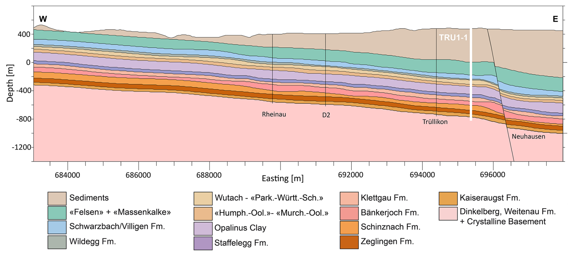
Figure 3 W–E cross-section of the geomechanical units passing through the Trüllikon borehole (Bold white line, TRU1-1) and a constant northing =277 548 m within the REF model domain. The depth is referenced to the sea level. Vertical exaggeration by a factor of 2.5 is applied to enhance the visibility of thin layers, such as the Wildegg Formation. The respective mechanical properties are shown in Table 1. Only depths down to −1400 m (b.s.l.) are shown for clarity, although the REF model extends to −2500 m (b.s.l.). The coordinate reference system used is CH1903.

The reference model (REF model) is rectangular, spanning 14.7 km E–W×14.8 km N–S laterally, and extending to a depth of 2.5 km below sea level ($\mathrm{b}.\mathrm{s}.\mathrm{l}.$). The upper boundary is defined by the local topography. In the siting region, S_Hmax orientation is 170 ± 11° according to the BO and DITF observations from the boreholes, in agreement with the regional trend (Nagra, 2013; Heidbach et al., 2025b). To align the model geometry with the S_Hmax orientation, the entire model domain is rotated by 10° counterclockwise from geographic north, such that its sides are parallel and perpendicular to the mean S_Hmax orientation (Fig. 2).

The present day geomechanically relevant layers were constructed using SKUA-GOCAD v19 software. Successive lithologies with comparable mechanical properties were combined (Table 1), eventually leading to 14 geomechanically different units in the REF model (Fig. 3). A total of seven faults and flexures, named Neuhausen, Uhwiesen, Wildensbuch, Marthalen-Rafz Flexure, Rheinau, D2, and Trüllikon, were implemented in the model (Fig. 2). These structures are modeled as contact surfaces, weakly interpreted from the regional 3D seismic sections, and are highly simplified for ease of implementation in the model. Here, simplification means merging much smaller segments interpreted on 3D seismics into larger, continuous fault planes to represent what is, in reality, a volumetric fault zone structure (Nagra, 2024a) (Figs. 2 and 3).

Both Neuhausen and Uhwiesen faults dip at 60° toward the northeast, while the others are vertical. Neuhausen is the only fault that has a stratigraphic offset, with a vertical displacement of approximately 50 m at the base of the Mesozoic units that decreases towards the surface (Nagra, 2002a, 2008, 2024d). The Marthalen-Rafz Flexur and Wildensbuch Flexur are monoclines that dominate the overlying Mesozoic strata in the siting region through a step-like bending rather than a discrete break in an otherwise dipping strata (Madritsch et al., 2024; Nagra, 2024c). Other than the Neuhausen fault, the remaining faults and flexures show no clear displacement but are included in the model as they represent the first-order geological structures of the ZNO siting region.

2.2 Reference model (REF model) setup

2.2.1 Model assumptions

The primary objective of the REF model is to reliably predict the present day stress state within the ZNO siting region. To achieve this, two key simplifying assumptions are made. First, transient effects such as time-dependent tectonic deformation or human-induced changes are neglected while considering only the stress contributions from the gravitational and tectonic forces. Since the model focuses on static stress field prediction, the rock volume is assumed not to undergo any transient deformation. Second, linear isotropic elasticity is assumed in the geomechanical units within the rock volume. This assumption simplifies the material parameters needed to explain the behavior of the rock under stress to just the Young's modulus which characterizes the elastic stiffness of the rock (E), Poisson's ratio which describes the lateral strain response (ν), and density (ρ) of each geomechanical unit. Throughout this work, we will refer to Young's modulus as stiffness and the contrast in Young's modulus as stiffness contrast. The equilibrium condition between the gravitational and the tectonic forces is governed by a second-order partial differential equation (PDE), with displacement as the field variable (Jaeger et al., 2007). Since this PDE cannot be solved analytically, a numerical solution is needed. Therefore, we use the Finite Element Method (FEM). FEM allows the use of unstructured meshes to represent the model volume, which is particularly useful when modeling complex geological features and variations in material properties (Mao, 2005; Henk, 2009).

Although several studies have shown that the stress state can be dominated by inelastic deformations once the elastic limits of the geomechanical units are exceeded (Smart et al., 2012; Pijnenburg et al., 2019; Yan et al., 2025), linear elasticity remains an appropriate first-order approximation for predicting the present day stress state in the ZNO siting region. This assumption is supported by several geological factors (Nagra, 2024d, c). The tectonic strain rates in northern Switzerland are extremely low, in the order of 1–3 $\mathrm{m}{\mathrm{Myr}}^{-\mathrm{1}}{\mathrm{km}}^{-\mathrm{1}}$, and the region is tectonically stable, with no significant deformation observed since the Miocene. More importantly, the observed differential stresses (S₁–S₃) within the geomechanical units range between 0.5–13 MPa, which are significantly lower than their measured uniaxial compressive strength limits of 33–180 MPa. Because the differential stresses in the geomechanical units are far below their peak strength, plastic deformation is not expected under the current stress state.

2.2.2 Model discretization

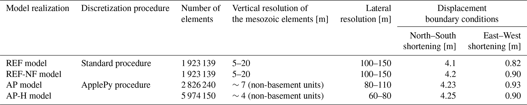
The model setup follows a standard series of steps, previously used in other regional geomechanical studies (Buchmann and Connolly, 2007; Reiter and Heidbach, 2014; Hergert et al., 2015; Ziegler et al., 2016; Rajabi et al., 2017a). The model volume is discretized into 3D elements, collectively referred to as a mesh. The 3D element resolution plays a significant role in capturing predicted stress variations, where smaller elements capture a higher spatial resolution but at increased computational cost (Ahlers et al., 2021, 2022). To ensure a reasonably accurate representation of each geomechanical unit, a minimum of three finite elements is used in the vertical direction. Accordingly, the top 13 geomechanical units, which are relatively thin (Fig. 3), are discretized with smaller element sizes vertically, whereas the deeper and thicker Basement unit is represented with larger element sizes in the vertical direction. A total of 1 923 139 tetrahedral and hexahedral finite elements are used, providing a high-resolution representation of the geomechanical units, with model resolutions varying from 100–150 m laterally and 5–20 m vertically. We use first-order elements in this study, and the discretization is done using Altair HyperMesh 2021 software package.

2.2.3 Mechanical rock properties and fault properties

Geological units with similar mechanical properties are grouped into the same geomechanical unit for simplicity. Each element in the mesh is assigned mechanical properties based on the corresponding geomechanical unit. The mechanical properties E [GPa], ν [–], and ρ [kg m⁻³] used in the models are derived from petrophysical logs and from uniaxial and triaxial compression tests performed on the core samples obtained from the TRU1-1 and MAR1-1 boreholes (Nagra, 2024c, b). From the distribution of values for each geomechanical unit, the median values (P50) are used for the model, summarized in Table 1. Geological faults are implemented as contact surfaces that can slip under mechanical loading as a structural response to stress conditions, depending on their frictional properties. In the REF model, contact surfaces are assigned a friction coefficient of 1 and a zero cohesion, values chosen to best represent the fault properties in the region (Nagra, 2024c).

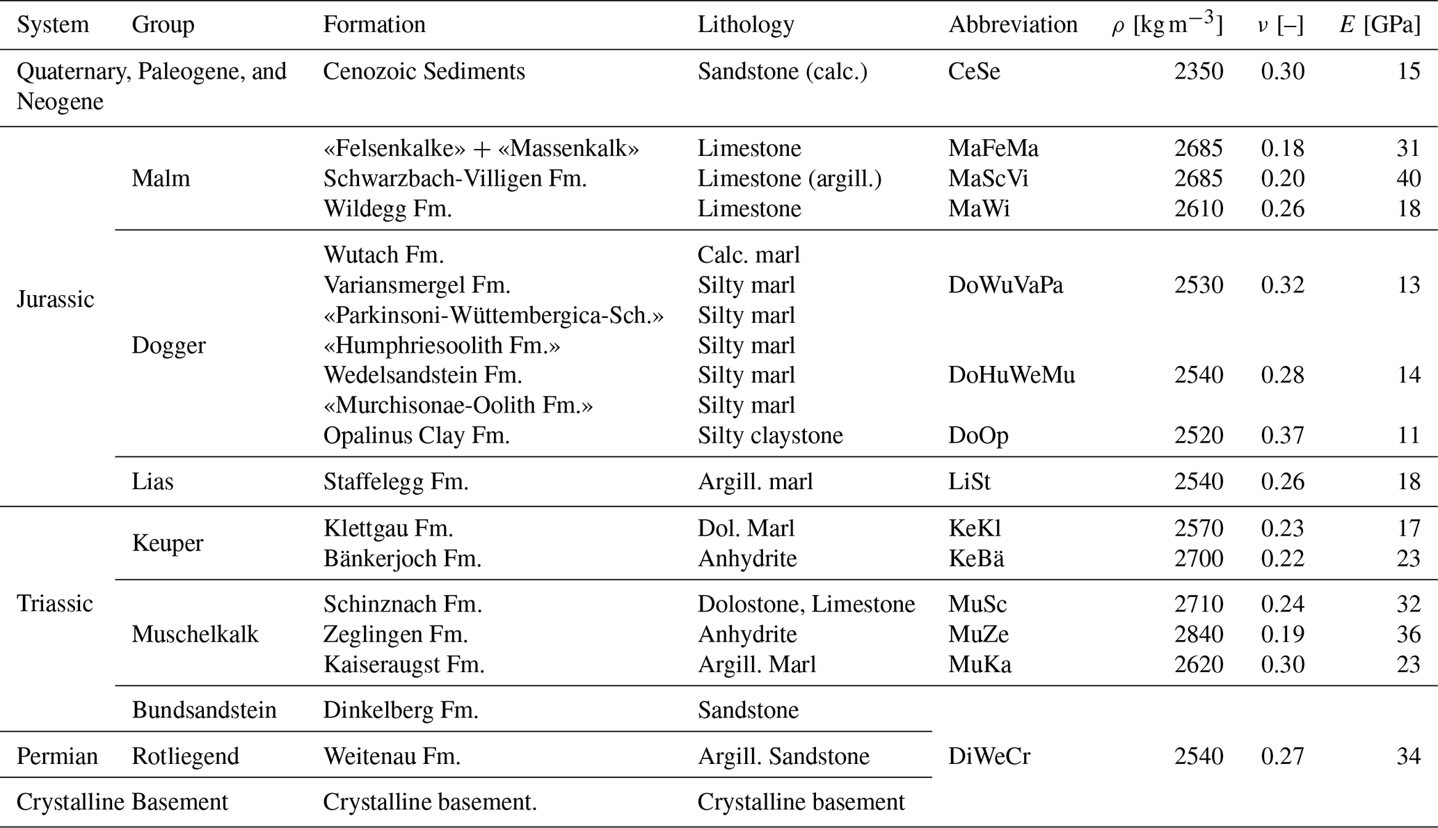
Table 1 Different geological formations with respective mechanical properties. The abbreviations are used solely to indicate the respective formations in the figures of this paper. Throughout the rest of this paper, the respective units can also be matched with the corresponding colors shown in Fig. 3 and with the abbreviations given here. Detailed information on the lithology is given in (Nagra, 2024c, b).

2.2.4 Model calibration

The present day stress state is computed by applying the gravitational forces and lateral displacement boundary conditions to simulate the tectonic loading from the geological history. These boundary conditions are chosen so that the modeled stresses best fit the measured horizontal stress magnitude data, a process known as model calibration (Reiter and Heidbach, 2014; Ziegler and Heidbach, 2020).

In total, we have 30 S_hmin and 15 S_Hmax magnitudes (Fig. 5). The S_hmin magnitude ranges (Fig. 5: red bars) are derived from the (MHF) tests and dry sleeve reopening (SR) tests (Desroches et al., 2021a, b, 2023; Nagra, 2024d) provide the basis to bracket the ranges for the S_Hmax magnitudes (Fig. 5: blue bars). However, the mean of these ranges was used for the model calibration.

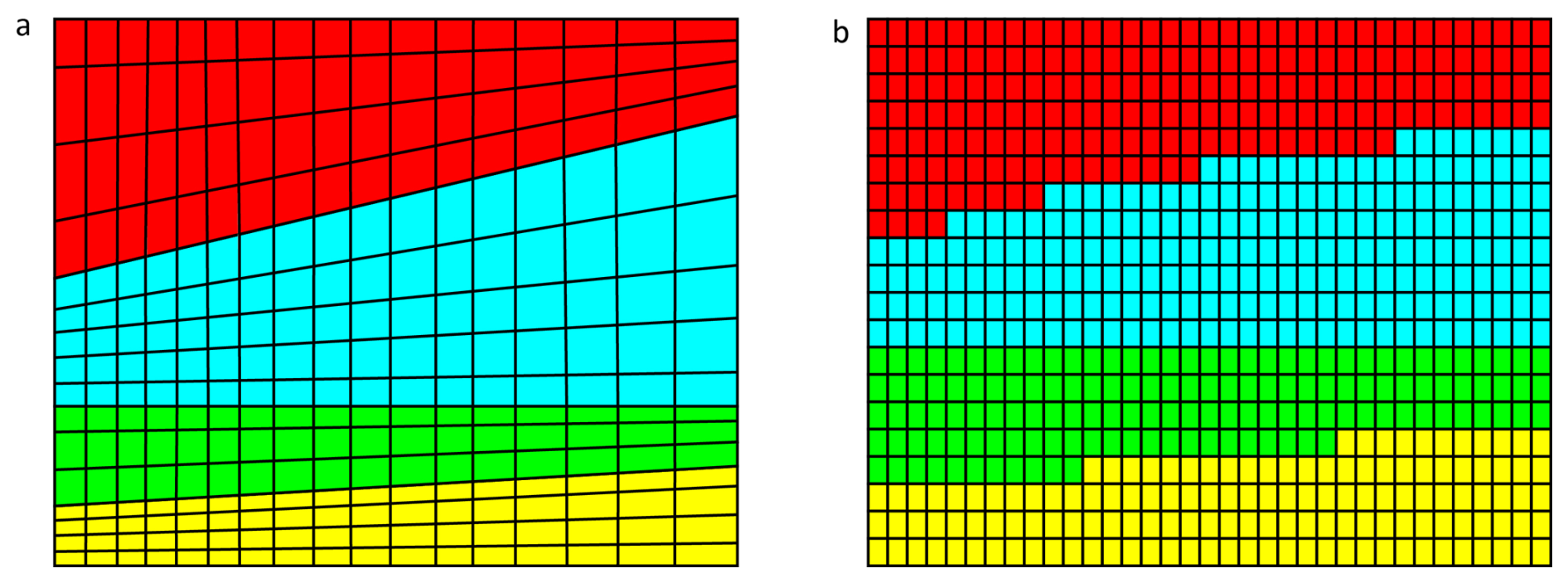
Figure 4 A conceptual visual comparison of (a) the standard procedure and (b) the ApplePy procedure for discretization and mechanical property assignment to geomechanical units. The four colors represent distinct geomechanical units, each with unique lithologies and mechanical properties.

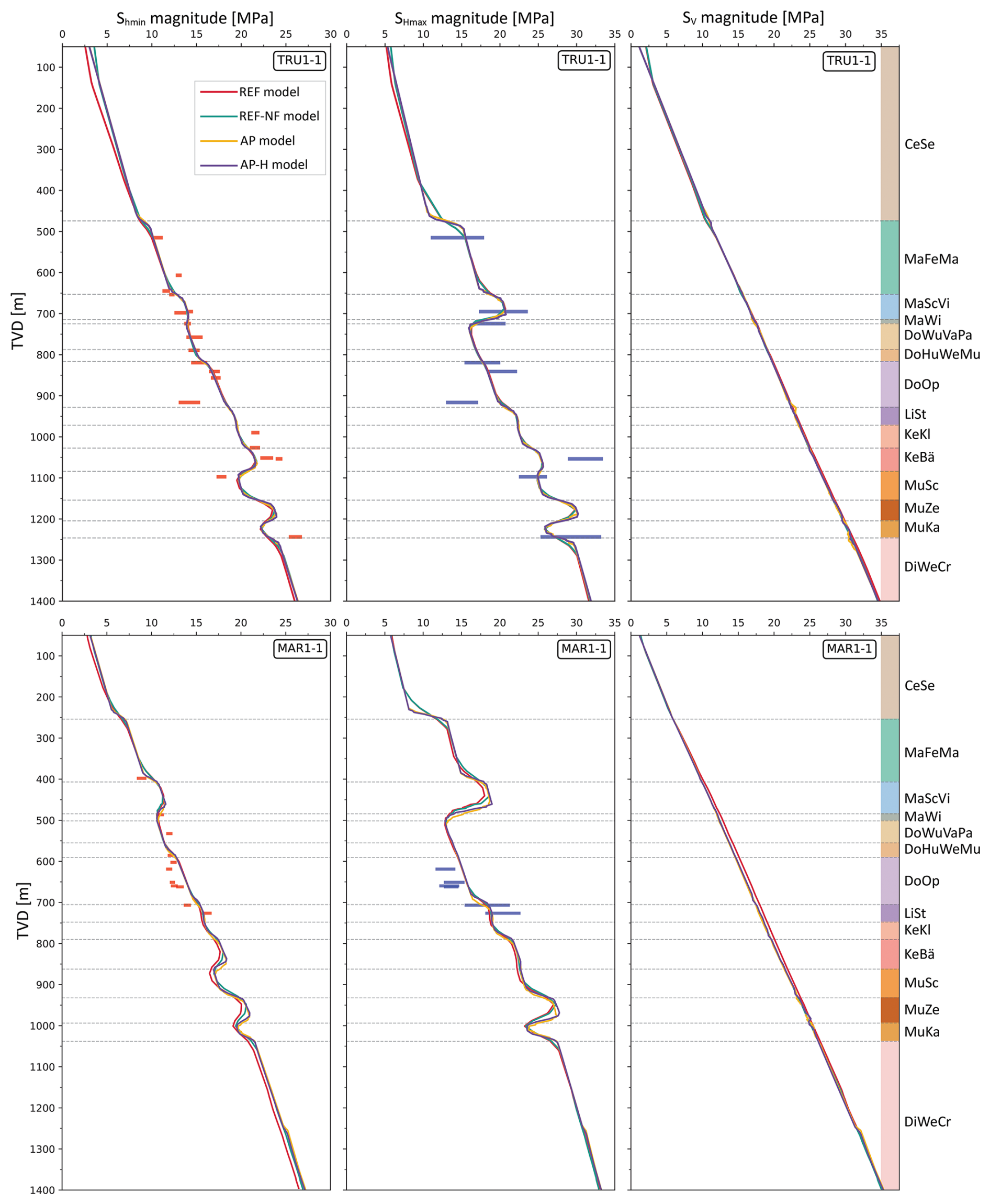
Figure 5 S_hmin magnitude, S_Hmax magnitudes, and S_V magnitude of all the model realizations with depth (TVD) along the borehole trajectories of TRU1-1 (top row) and MAR1-1 (bottom row). The red and blue horizontal bars show the measured in-situ stress magnitude data of the S_hmin and S_Hmax, with lengths indicating their individual uncertainty (Nagra, 2024d, c). The geomechanical units are represented by their respective colors and abbreviations, consistent with Fig. 3 and Table 1.

The model calibration is done using the PyFast Calibration tool (Ziegler and Heidbach, 2021), which uses a linear regression-based algorithm to compute the best-fit lateral displacement boundary conditions by minimizing the differences between the modeled and measured horizontal stress magnitudes. The resulting best fit for the boundary conditions of the model volume was found to be a total shortening of 0.82 m applied in the east–west direction, and 4.2 m in the north–south direction. Displacements parallel to the boundaries are permitted on all lateral faces of the model. At the base, vertical displacement is constrained to zero, while horizontal displacement is permitted; the model top remains fully unconstrained. The numerical solution is computed using the Simulia Abaqus v2021 finite element solver. The results are analyzed using Tecplot 360 EX 2023 R2 along with the Geostress v2.0 add-on library (Stromeyer et al., 2020).

3 Model set-up of 3D geomechanical numerical models without fault representation

3.1 Model discretization strategies

Removing the fault implementation from the 3D models allows us to use different model discretization strategies, which in turn significantly accelerates the model setup and stress prediction workflow. Using two different discretization strategies, we developed three additional fault-agnostic 3D geomechanical numerical models. The reference model and the three fault-agnostic models are then compared to quantify the spatial influence of faults on the far-field stress state. In our study, the time required to build a model was reduced from approximately two months for the reference model, the model that includes contact surfaces, to just two days for the fault-agnostic models.

The standard procedure discretizes each geomechanical unit individually using the definition of its top and bottom interface surfaces, and later connected by matching the nodes along the common interfaces. Each element of the unit is assigned to the appropriate mechanical properties (Fig. 4a) directly from the stratigraphic definition. While this approach results in a smooth unit boundary, it requires substantial manual effort and is particularly time-consuming when working with models containing many geomechanical units.

In order to simplify the setup and discretization procedure of the fault-agnostic models, we use ApplePy (Automatic Partitioning Preventing Lengthy Manual Element Assignment), a Python-based tool that automates the discretization and element property assignment process (Ziegler et al., 2020). The entire model volume is discretized in a single step as a largely homogeneous mesh, ignoring both lithological interfaces and fault structures. ApplePy uses the depth values of the stratigraphic boundaries to decide which element belongs to which lithological unit/geomechanical unit (Fig. 4b). Although this approach introduces step-like transitions at unit boundaries which looks optically unrealistic, it significantly reduces the meshing time, especially for large or complex models, like the REF model without compromising the stress prediction capability of the final 3D geomechanical numerical models, as discussed in Sect. 4.

Table 2 Summary of technical specifications for all model realizations used in this study. Reported vertical resolutions refer only to the Mesozoic units and are approximate for the ApplePy models due to depth-dependent variation. Minor differences in displacement boundary conditions reflect the presence of contact surfaces in the reference model, which allow elastic energy dissipation that is absent in the fault-agnostic models. The boundary conditions are compressional in nature.

3.2 Model realizations and configurations

Building on the discretization strategies described in Sect. 3.1, three fault-agnostic 3D geomechanical numerical model realizations were developed. The three fault-agnostic 3D geomechanical numerical models follow the general model workflow of the REF model, i.e., the model parameterization and calibration are the same (Sect. 2.2), along with the same model extents (Sect. 2.1). They are calibrated to the same dataset of 45 horizontal stress magnitude measurements used for calibrating the REF model. The only differences lie in the model discretization strategies (Sect. 3.1) and finite element resolution. Out of these three models, one is set up using the standard procedure, and two are set up using the ApplePy procedure. Table 2 presents the technical details on the number of elements and spatial resolution of each model used, along with the corresponding best-fit displacement boundary conditions obtained after applying FAST Calibration tool. The brief description of the three fault-agnostic models is:

• REF-NF model: Derived directly from the REF model with identical geometry, mesh and mechanical property assignments but with faults removed. Contact surfaces are eliminated, and opposing nodes are equivalenced, except for the Neuhausen Fault, where a 50 m lithological offset prevents node equivalencing. In this case, slip is prevented by assigning an artificially high friction coefficient of 50.

• AP model: Maintains the same extents and mechanical properties as the REF and REF-NF models but uses ApplePy for property assignment to the elements. It does not incorporate faults and has approximately 50 % more elements than the REF and REF-NF models.

• AP-H model: A higher resolution version of the AP model, with twice the number of elements. All the other features of the model are the same as the AP model.

4 Results

4.1 Stress magnitudes along borehole trajectories

The resulting predicted stress magnitudes from all the model realizations are presented together with the measured S_hmin (red bars) and estimated S_Hmax (blue bars) magnitude ranges along the TRU1-1 and MAR1-1 borehole trajectories in Fig. 5. In general, the predicted horizontal stress magnitudes from the REF model align reasonably well with the measured stress ranges across different geomechanical units. However, some discrepancies are present, particularly in the Klettgau and Bänkerjoch formations, where the REF model underestimates S_hmin magnitudes, and in the Schinznach formation, where S_hmin magnitude is overestimated. These deviations arise because, for the model calibration, the REF model uses P50 (median) horizontal stress magnitude values despite the MHF tests resulting in ranges (red and blue bars in Fig. 5). Therefore, the stress predictions may vary from the assumed P50 value at a particular point in the subsurface. The vertical stress magnitude (S_V) is calculated from the weight of the overlying rock mass, considering the densities of the individual lithologies. From Fig. 5, it can be seen that S_V increases linearly with depth.

The predicted results from all the model realizations, regardless of fault implementation or exclusion, also align well with the measured horizontal stress magnitude ranges along both borehole trajectories across different geomechanical units, and are consistent with the REF model. Minor but negligible differences of <1 MPa in the S_Hmax magnitudes can be found at ∼475 m (t.v.d) along the TRU1-1 borehole and at ∼250 m (t.v.d) along the MAR1-1 borehole in the AP and AP-H models (Fig. 5). This is likely due to a high stiffness contrast between the Cenozoic sediments (E= 15 GPa) and Felsenkalke + Massenkalke (E= 31 GPa) units, the transition boundary of which is differently discretized due to ApplePy usage. A similar difference can be found at the Zeglingen Fm. (E= 36 GPa), Kaiseraugst Fm. (E= 23 GPa) and the Dinkelberg, Weitenau Fm. and Crystalline basement (E= 34 GPa), which is also due to the widely varying stiffness contrasts.

Stiffer formations such as the Schwarzbach-Villigen Fm., Zeglingen Fm., and the basement have broader stress ranges in the measured data due to their statistically larger stiffness variability, while weaker formations like the Opalinus Clay exhibit narrower, more consistent stress distributions. Moreover, stiffer layers shield the weaker layers above and below, reducing stress variability in these formations. In short, Fig. 5 clearly indicates that the differences between the profiles from all the models are smaller than the measurement errors, represented by the length of the horizontal red and blue bars, and that the differences between the fault agnostic models and the REF model are insignificant. The variation of S_V magnitude with depth is consistent across all the model realizations, with differences <0.05 MPa observed between the models using ApplePy and the standard procedure.

The AP and AP-H models yield identical results. This indicates that increasing model resolution would not significantly improve stress predictions in our study and that the resolution of the AP model is already sufficient. This rules out resolution effects within the ApplePy models on the predicted stress magnitudes with respect to the REF model.

4.2 Model results along a vertical cross-section and a horizontal layer

4.2.1 Horizontal differential stress (S_Hmax−S_hmin)

Along the W–E cross-section through borehole TRU1-1, the horizontal differential stress (S_Hmax−S_hmin) of the four models displayed in Fig. 6a–d shows only small differences, except near the contact surfaces where noticeable localized stress concentrations in the REF model occur. Similar result shows up when comparing the values of S_Hmax-S_hmin along the mean Opalinus clay layer from the REF model (Fig. 6e) with those of REF-NF model (Fig. 6f). To quantify the difference of the three fault-agnostic models w.r.t the REF model, Fig. 7a–c displays the difference in the horizontal differential stress Δ(S_Hmax−S_hmin) between the models. The values of Δ(S_Hmax−S_hmin) exceed ±2 MPa only within 100 m of the fault. Beyond approximately 200 m from the faults, Δ(S_Hmax−S_hmin) across all models becomes more similar to each other, and differences relative to the REF model typically remain below ±0.4 MPa. As the distance from the faults increases, the value of Δ(S_Hmax−S_hmin) differences rapidly decreases.

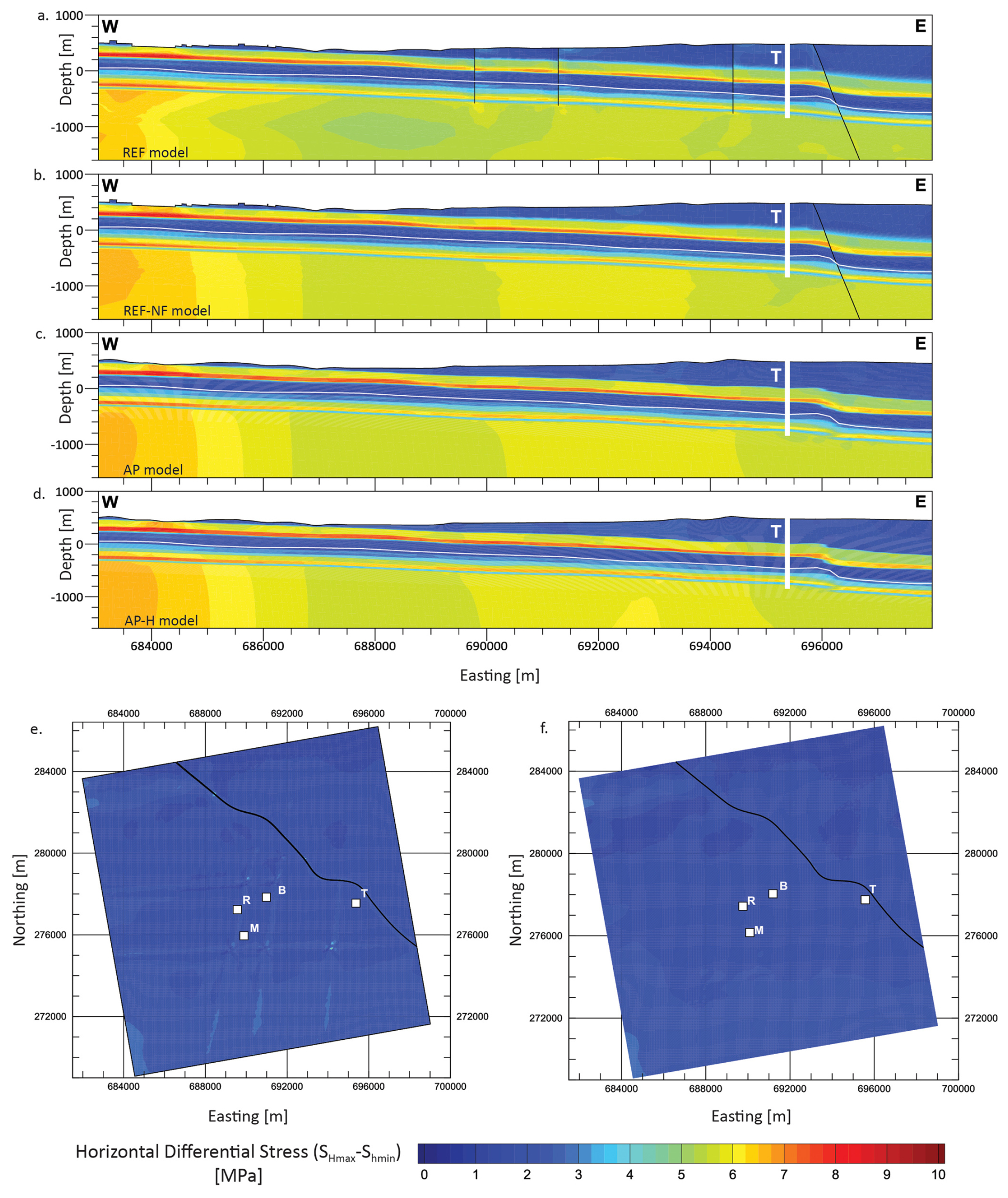
Figure 6 (a–d) Modelled horizontal differential stress (S_Hmax−S_hmin). (a–d) W–E cross section (brown line in Fig. 2) through the TRU1-1 borehole (white vertical bar) with depths referenced to below sea level (b.s.l.). The location of faults is indicated by black lines. (e, f) Mean Opalinus Clay layer of the REF and REF-NF model, indicated by the white lines on the W–E cross sections. Capital letters indicate the location of the four boreholes TRU1-1 (T), BEN (B), MAR1-1 (M), and RHE1-1 (R).

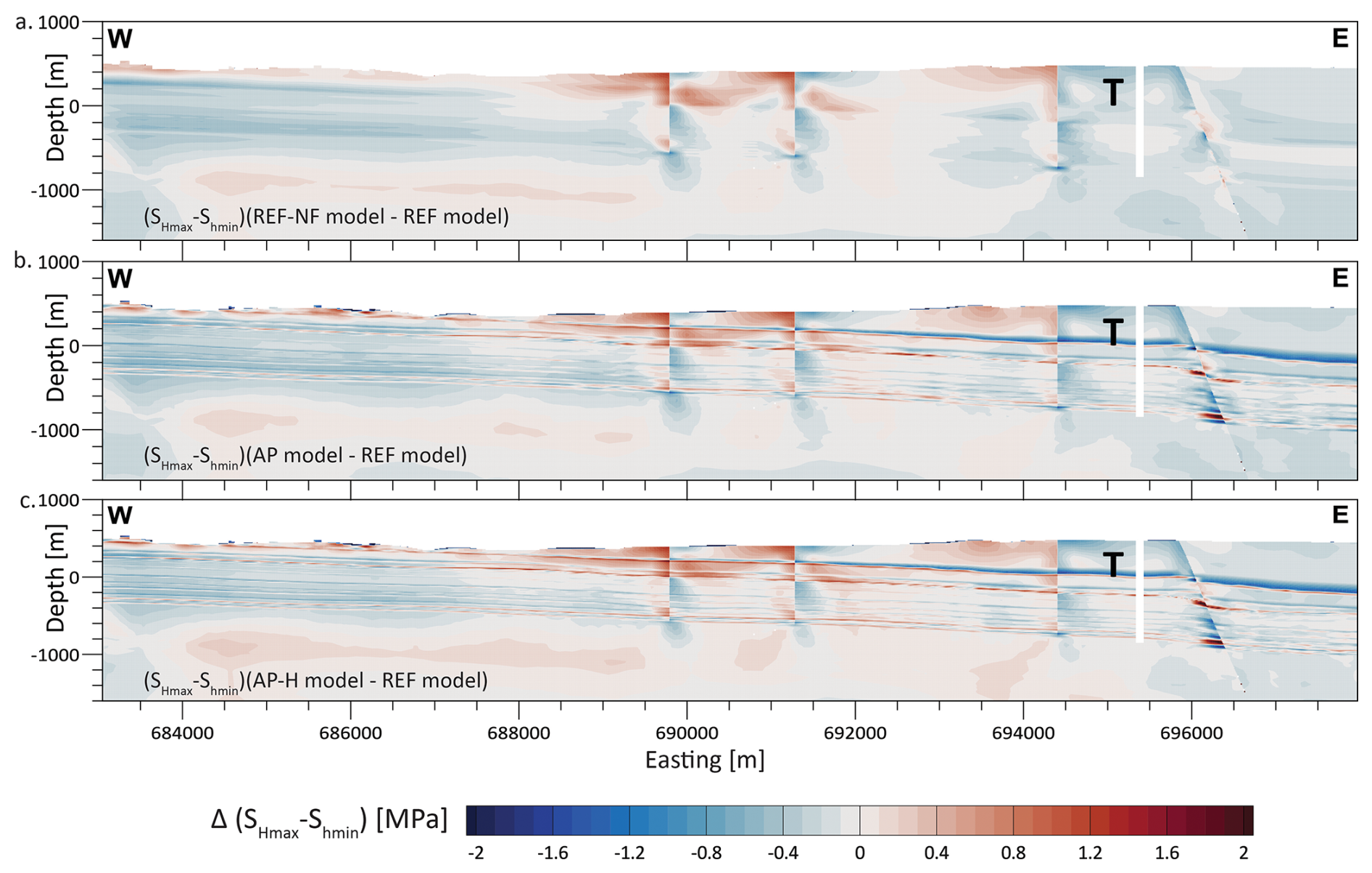
Figure 7 (a–c) Difference of S_Hmax−S_hmin between the models without faults and the REF model with active faults along the same cross-section as in Fig. 6. The cross-sections show the difference with respect to the REF model and are indicated at the bottom left of each slice. Although faults have not been directly indicated on the cross-sections, the location of the faults can be visually seen as sudden lateral changes in an otherwise continuous change in Δ(S_Hmax−S_hmin).

In addition to the spatial proximity to contact surfaces, the variation of S_Hmax−S_hmin depends on the stiffness of the geomechanical units. In specific Mesozoic units characterized by lower stiffness, such as from the Wildegg Fm. of the Malm Group to the Klettgau Fm. of the Keuper group, and the Kaiseraugst Fm. of the Muschelkalk group (Table 1), the S_Hmax−S_hmin typically is <3.5 MPa. In contrast, units with high stiffness can exhibit S_Hmax−S_hmin exceeding 7 MPa, such as in the «Felsenkalke» + «Massenkalk» and the Schwarzbach-Villigen Fm. of the Malm group, Schinznach and Zeglingen Fm. of the Muschelkalk group and the Dinkelberg Fm., Weitenau Fm. and Crystalline basement ( Table 1). This trend is expected, as lower stiffness materials accommodate deformation more readily, resulting in lower differential stresses, whereas stiffer units resist deformation, leading to higher differential stresses. The Opalinus Clay layer has a Young's modulus of 11 GPa, which is relatively low compared to the other geomechanical units present in the siting region. The adjacent stiffer geomechanical units act as stress-bearing members, effectively shielding the soft layer and further reducing the stress magnitudes concentrated within it. The S_Hmax−S_hmin in the mean Opalinus Clay layer, as predicted by the models, is <2 MPa irrespective of fault inclusion or exclusion from the model (Fig. 6e and f).

A particularly notable observation is that the differential stress near the Neuhausen fault remains relatively comparable across all models when compared to the magnitude of differences in S_Hmax−S_hmin at other contact surfaces. Despite the Neuhausen fault being either fully removed or mechanically disabled via a high friction coefficient, the differential stress pattern across the 50 m offset between the footwall and the hanging wall is well replicated in the AP and the AP-H models in Fig. 6a–d. This is attributed to the abrupt contrast in mechanical properties across the Neuhausen Fault (Fig. 3; Table 1), which effectively mimics the local stress response, even in the absence of explicit fault representation.

4.2.2 S_Hmax orientation

Along the same W-E cross-section as in Fig. 6a–d, the S_Hmax orientation of the four models is displayed in Fig. 8a–d, and the variability of the S_Hmax orientation w.r.t the REF model is displayed in Fig. 9a–c. Figure 8e–f show the variability of S_Hmax orientation along the mean Opalinus clay layer from the REF model and the REF-NF model respectively.

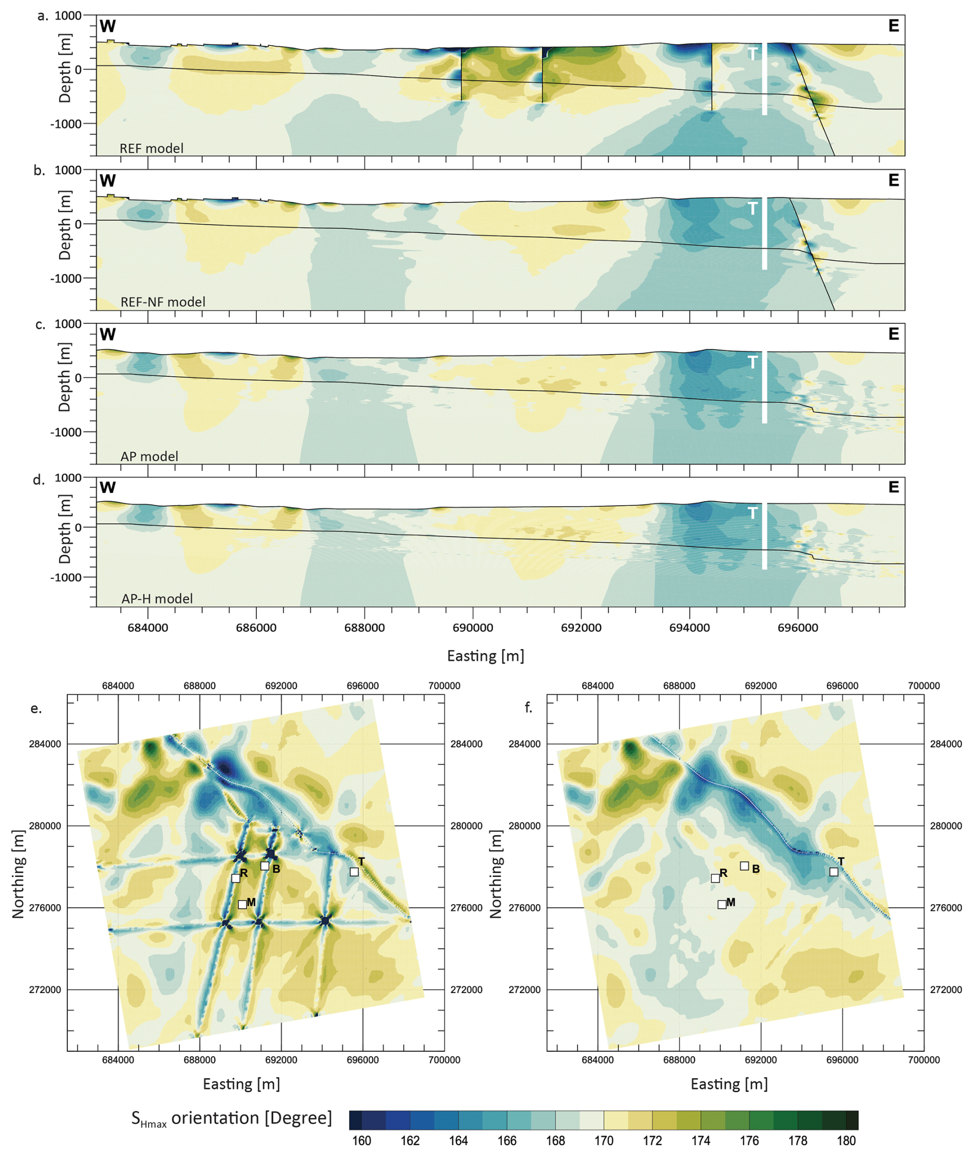
Figure 8 Absolute S_Hmax orientation. (a–d) W–E cross-section through borehole TRU1-1 (T) indicated with the white vertical bar. (e, f) Mean Opalinus Clay layer of the REF and REF-NF model, indicated by the black lines on the W–E cross sections. Capital letters indicate the location of the four boreholes TRU1-1 (T), BEN (B), MAR1-1 (M), and RHE1-1 (R).

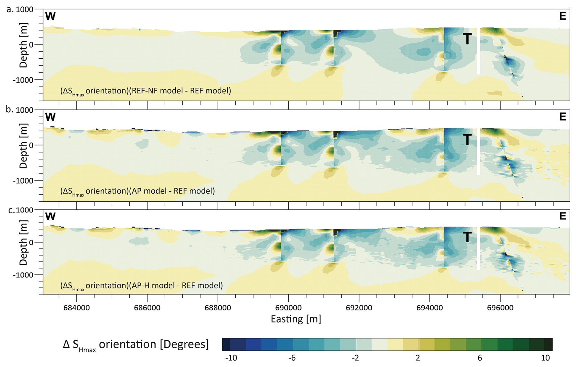
Figure 9 (a–c) Difference of S_Hmax orientation between the models without faults and the REF model with active faults along the same cross-section as in Fig. 7. The cross-sections show the difference with respect to the REF model and are indicated at the bottom left of each slice. Although faults have not been directly indicated on the cross-sections, the location of the faults can be visually seen as sudden lateral changes in an otherwise continuous change in Δ S_Hmax orientation.

The largest S_Hmax orientation variability is reoriented more within a distance of 100–200 m around the contact surfaces, similar to the observations of Δ(S_Hmax−S_hmin). At this distance, differences greater than 6° w.r.t. the REF model are observed. These differences tend to reduce to less than ±2° at lateral distances greater than 500 m from the contact surfaces. Within the near-field zone, which is <300 m from the contact surfaces, stress concentrations are probably artifacts arising from the numerical resolution limit. This shift in S_Hmax orientation can also be observed in Fig. 8e–f along and near the contact surfaces. Even under a hypothetical assumption that the observed variations are entirely fault-induced, the current stress indicator techniques cannot resolve S_Hmax variations within 10°. Therefore, these differences can be considered insignificant and non-resolvable. Finally, increasing model resolution does not change our results, as seen when comparing the AP and AP-H model results in Figs. 8 and 9.

4.3 Quantification of the lateral extent of fault-induced stress changes

To better quantify the impact of faults on stress, we interpolated the results of the four models on a SW-NE oriented horizontal line at 300 m (b.s.l.) crossing five of the seven faults (Fig. 10a–c). To improve readability, the results from the AP model were not plotted, as it is clear from Figs. 5, 7, and 9 that the AP and AP-H model results are almost identical.

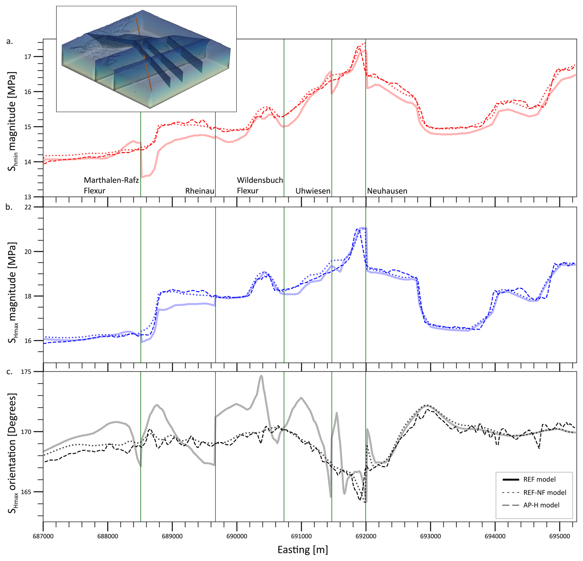
Figure 10 Magnitudes of S_hmin and S_Hmax, and the S_Hmax orientation along a SW–NE horizontal profile at 300 m (b.s.l.), shown in the 3D figure as a red line. Green vertical lines with the respective fault names denote the location where the profile crosses the modelled faults.

The S_Hmax and S_hmin magnitudes of different model realizations largely overlap each other along the horizontal line. A difference of ∼0.5 MPa is observed in S_Hmax magnitude (Fig. 10b), and ∼1 MPa is observed in the S_hmin magnitudes (Fig. 10a) between the REF model and the fault-agnostic models, within ∼500 m of the faults. However, these differences are less than the widths of the stress magnitude data, which in turn, represent the uncertainty of the measurements (Fig. 5). In general, the horizontal stress magnitudes from the REF model have an abrupt change in the vicinity of the faults, deviating from the continuous trend followed by other model realizations. The differences in the S_Hmax magnitudes reduce to <0.2 MPa beyond a distance of about 500 m from the fault. The differences in the S_hmin magnitudes follow the same pattern as the S_Hmax magnitude, and also reduce beyond a distance of about 500 m away from the fault.

Similarly, the S_Hmax orientation of the REF model shows negligible deviations of <2° in the undisturbed rock volume, away from the faults, and a deviation of 2–6° up to 1 km from the modeled faults (Fig. 10c). According to the quality ranking scheme of the S_Hmax orientation from the World Stress Map, the A-quality data, data of the highest quality, has a standard deviation of ±15° (Heidbach et al., 2025a). Even S_Hmax orientations derived from the DITF and BO in the MAR1-1 and TRU1-1 boreholes exhibit standard deviations of approximately ±11°. Considering this, the orientation deviations seen in Fig. 10c are not resolvable and well below the uncertainties of the in situ indicators.

Near the Neuhausen fault, there is a localized abrupt change in the horizontal stress magnitudes within ∼100 m on either side of the modelled fault for all the model realizations. An important observation is that this abrupt change occurs not only in the REF model but also in the models without any faults. These stress changes are primarily controlled by the lateral stiffness contrasts due to the offset and not by the mere presence of the faults.

Overall, the differences are <0.2 MPa in stress magnitudes and <2° in S_Hmax orientations beyond 1 km from the fault, which is far less than the uncertainties of the horizontal stress magnitude data from the MHF and the SR tests, as well as the stress indicators for the S_Hmax orientation from the boreholes. Even in a conservative approach, it is clear that the effect of faults on the stress field is within about 1 km from the fault core. This conclusion aligns with the findings by Reiter et al. (2024), who, through generic model studies, found that significant stress changes due to faults only occur within a distance of a few hundred meters, partly up to 1 km next to the fault.

5 Discussion

5.1 Comparison with observed S_Hmax orientation data

The S_Hmax orientation is the most widely available characteristic of the reduced stress tensor. It is also the easiest to analyze because it can be averaged and visualized with respect to the fault on stress maps (Fig. 1) (Yale et al., 1993, 1994; Yale and Ryan, 1994; Yale, 2003; Rajabi et al., 2017c; Heidbach et al., 2018). The S_Hmax orientation can be determined from different stress indicators, such as from direct borehole-based indicators, earthquake focal mechanisms, geological indicators, or passive seismic methods (Amadei and Stephansson, 1997; Zang and Stephansson, 2010; Heidbach et al., 2025a). Among these, direct borehole-based indicators such as borehole breakouts (BOs), drilling-induced tensile fractures (DITFs), and hydraulic fracturing (HFs) are commonly considered to be the most reliable (Bell, 1996a; Zang and Stephansson, 2010).

In the ZNO study region, 11 S_Hmax orientation data records are available from HFs, DITFs, and BOs. The mean S_Hmax orientation from these data is 170° with a standard deviation of ±11° (Nagra, 2024d, c; Heidbach et al., 2025b). The individual standard deviation of each data record is between ±9 and ±19°, indicating that rotations $<\pm \mathrm{11}$° cannot be resolved. As the differences between the REF model and the three fault-agnostic models, as displayed in Fig. 9, are smaller than ±10°, the potential impact cannot be resolved with any stress indicator. Furthermore, most of the rotations observed are located close to the fault. At a distance of 1000 m from a fault, the rotation is $<\pm \mathrm{2}$° and thus clearly below the uncertainties of any measurement.

The stress regime of the rock volume, by itself, would not have an influence on the S_Hmax orientation. A rotation of S_Hmax orientation would primarily be driven by the horizontal differential stresses, i.e., the greater the horizontal differential stresses, the lesser the possibility of any rotation in the S_Hmax orientation (Bell, 1996a; Yale, 2003; Reiter et al., 2024).

The 1 km spatial distance limit can also be confirmed by viewing the S_Hmax orientation from the boreholes in correlation with their distance from the nearest faults. The TRU1-1 borehole is less than 1 km from the Neuhausen fault. Similarly, the MAR1-1 and RHE1-1 boreholes are closest to the Rheinau fault. The average S_Hmax orientation from the BO, DITF, and HF is ∼165° along the TRU1-1 borehole, ∼175° along the MAR1-1 borehole, and ∼172.5° along the RHE1-1 borehole (Nagra, 2024d, c). Comparing the S_Hmax orientation values from these three boreholes to the regional S_Hmax orientation value of 170 ± 11° already strengthens the argument that the faults have minimal effects on S_Hmax orientation even at a distance of less than 1 km.

5.2 Impact of varying fault friction coefficient of the implemented faults

In geomechanical modelling, the fault strength is commonly characterized by its friction coefficient (μ) and cohesion (Brandes and Tanner, 2020). In most geological settings, the friction coefficient varies between 0.6 and 1.0 in reservoirs with depths where normal stresses are <200 MPa on a pre-existing fracture plane (Byerlee, 1978; Zoback and Healy, 1984). In stark contrast, significantly lower friction coefficient values are found in geological settings with extremely weak lithologies, overpressured fault cores, and in faults with very large offset and/or high slip rates (Morrow et al., 1982, 1992; Di Toro et al., 2011; Hergert et al., 2011; Li et al., 2022). Cohesion varies with different lithologies, but for pre-existing faults, it is commonly assumed to be zero. In general, the value of the friction coefficient varies between 0.4 and 0.8, and is standardly taken as 0.65 (Hawkes et al., 2005; Kohli and Zoback, 2013). In northern Switzerland, taking the lithology and the geological setting into consideration, the values of apparent fault friction coefficient also range from 0.6 to 1.0, and very rarely to 0.4 (Kastrup, 2002; Viganò et al., 2021). Kastrup (2002) states that the apparent fault friction value of 0.2 is extremely rare in Switzerland and only occurs at depths of more than 10 km.

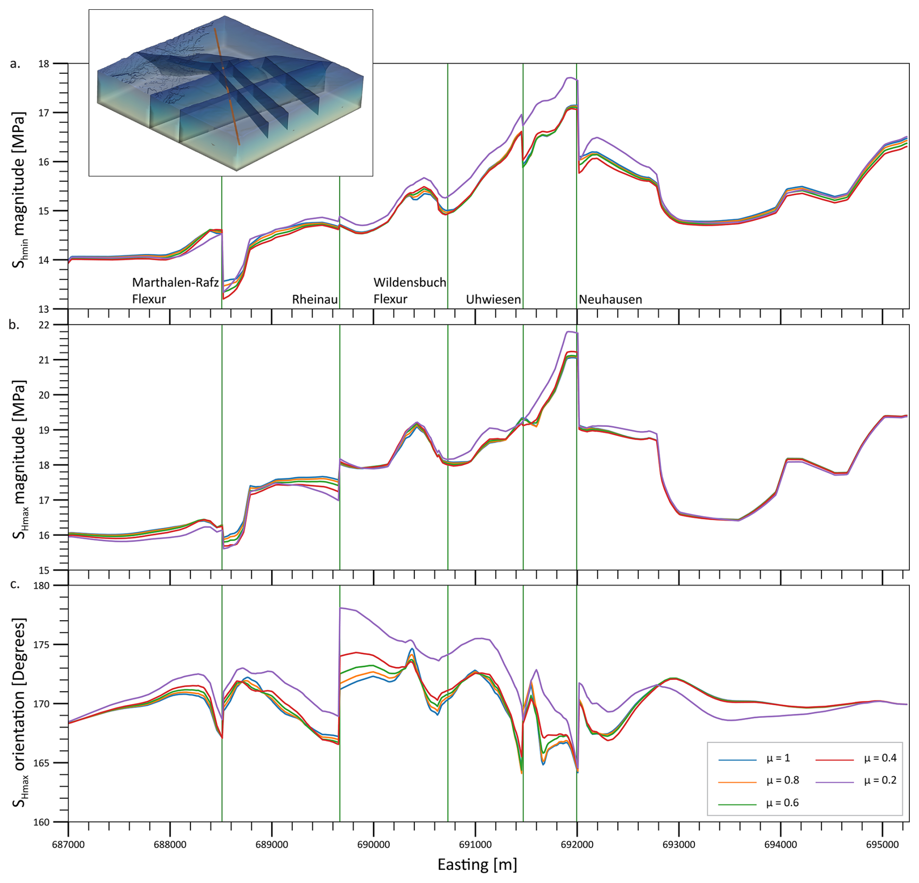
Figure 11 Impact of friction coefficient (μ) on the stress tensor components. The model used here is the REF model. The results are plotted along the SW–NE horizontal profile at 300 m (b.s.l.), shown in the 3D figure as a red line. Green vertical lines with the respective fault names denote the location where the profile crosses the modelled faults.

We investigate the effect of varying the friction coefficient of the contact surfaces on the predicted in situ stress state and recalibrate the REF model with a different friction coefficient. The results of stress magnitudes and orientation from friction coefficients 0.2, 0.4, 0.6, and 0.8 are compared to the friction coefficient of 1.0, the value we use in the REF model (Fig. 11). We see that changes in friction coefficient do not significantly affect our model results beyond lateral distances of 1 km. Even within 1 km from the faults, the horizontal stress magnitudes have observable variations of <1 MPa and <5° for the S_Hmax orientation variations. These variations reduce to <0.25 MPa in both minimum and maximum horizontal stresses, and <2.5° in the S_Hmax orientation beyond 1 km from the faults. The maximum variations, still far less than the uncertainties in the in situ stress data of the stress magnitudes and resolvable S_Hmax orientations, occur at a friction coefficient of 0.2. For the other values of the friction coefficient, the results are very much comparable to the REF model, with a friction coefficient of 1. This is to show that changing the friction coefficient has a negligible effect on the predicted stresses in our model. Minor amounts of slip, in the order of a few tens of cm, occur along the faults in the REF model during the application of boundary conditions. However, the stress change along the fault due to this slip is expected to be far less than the much larger background stresses and the differential stresses. Therefore, the minor slip occurring along the contact surfaces does not influence the overall stress field analysis.

These findings are in line with the results from the generic studies by Homberg et al. (1997) and Reiter et al. (2024), who studied the impact of variable friction coefficient on astress tensor and found that lower values of friction coefficient lead to a higher stress perturbation near the modelled fault. This is also seen in Fig. 11 and is because of possible decoupling at the fault and consequently a better dissipation of stress at the faults, facilitated by lower friction coefficients. The studies also showed that this effect is limited to a distance of 1 km from the fault zone.

5.3 Dependence of the modeling results on fault implementation

Faults in the REF model are represented as contact surfaces, a common and effective approach for large-scale geomechanical simulations. Using contact elements to model faults seems to be a reasonable simplification for large, field-scale reservoir models, where the actual width of the fault core is much smaller than the overall size of the model. Hence, contact surfaces are computationally efficient for reservoir-scale models where actual fault zone widths are negligible compared to model dimensions (Caine et al., 1996; Treffeisen and Henk, 2020). Since our interest is on reservoir scale, alternative fault representation using, e.g. continuous rectangular finite element grid, or a continuous curvilinear finite element grid in a homogenized continuum (Henk, 2009, 2020) is not used in our study. Furthermore, the results from Treffeisen and Henk (2020) and Reiter et al. (2024) show that the stress and strain perturbations from different technical fault implementations vary only within a few tens to a few hundred meters from the fault representation. As we focus only on the far-field stress state, it can be safely assumed that the choice of fault implementation approach does not significantly affect the far-field results.

Although a numerical value does not exist for what is universally defined as far-field stresses, our model indicates that at a distance of >500 m from the faults, the impact of the faults on the stress field is clearly smaller than the uncertainty of the model itself and smaller than the expected variability of the stress field. As seen in Fig. 10, the influence of faults on the stress field is limited to within 1 km from the contact surfaces. Beyond this distance, the choice of the fault representation approach would have no significant impact on the predicted in situ stress state.

5.4 Limitations of the study's results and future outlook

In the REF model, the faults, represented by contact surfaces, are simplified and a unified representation of numerous small fault patches that were interpreted from the 3D seismic interpretation. This simplification is necessary for an easier and reasonable representation of fault structures and the consequent computational simulation feasibility of the model. However, the reality is more complex. In the subsurface, faults often occur in clusters and display heterogeneous geometry, composition, and structure (Tanner and Brandes, 2020). Large faults are often accompanied by zones of secondary faults, which can extend the spatial influence of faults on the stress state. Small fault segments of the primary fault and the associated secondary faults can lead to a higher stress concentration along the fault surfaces, complicating the interaction between faults and the in situ stresses (Jones, 1988; Maerten et al., 2002). A single fault may also have complex geometry with multiple bends (Saucier et al., 1992; Roche et al., 2021), increasing its influence on stresses compared to the planar faults.

Our study focuses on a reservoir scale, in the order of a few km, to predict present day stress variation in the area of interest. While seven faults were implemented in the REF model, many more fractures or joints exist in reality but cannot be resolved at our current lateral resolution of approximately 70–100 m, and the available structural geological data. Including these would significantly increase the element count and computational demand, far beyond the scope or need of most studies. It is important to emphasize that the focus of our results is only the far-field present day stresses, and in an intact and undisturbed rock volume.

While previous studies have documented significant stress rotations near fault tips, they also emphasize that these perturbations are typically localized, rarely extending beyond a few hundred meters from the termination point (Homberg et al., 1997; Nicol et al., 2020). Our findings are in general agreement with this observation. In our model, fault tips ending within the Mesozoic sediments indeed exhibit localized stress concentrations and enhanced stress rotations. However, because these effects are spatially restricted, they do not significantly alter the regional stress field predicted by the fault-agnostic models at distances greater than a few 100 m from the structural discontinuities.

Extreme cases exist where large-scale faulting separated the crust into distinct fault blocks, each having an independent S_Hmax orientation between adjacent fault blocks of the same field (Yale et al., 1994; Yale and Ryan, 1994; Bell, 1996b; Kattenhorn et al., 2000; Hergert and Heidbach, 2011; Hergert et al., 2011; Li et al., 2019; Qin et al., 2024). While complex stress patterns and large S_Hmax rotations have been reported for major fault systems such as the Møre–Trøndelag Fault Complex and the San Andreas Fault, these systems differ fundamentally from the Alpine Foreland Basin in terms of tectonic setting, fault displacement magnitude, and fault frictional properties (Zoback et al., 1987; Pascal and Gabrielsen, 2001; Roberts and Myrvang, 2004). In particular, the large offsets and anomalously low friction coefficients reported for these systems are not representative of the fault conditions in northern Switzerland. But, as seen in our study region, if the Mesozoic sediments are not massively faulted or fractured, have sufficiently large differential stresses, and are located in an intraplate Foreland Basin setting, it could be expected that the impact of faults on the stress state would only be within 1 km from the fault zone. However, further investigation is needed for other geological settings, with different lithologies such as salt domes, anhydrite, or crystalline rock formations, or regions where faults exhibit more complex geometry with more curvature/bends, or with extremely large total offsets and high slip rates, to confirm the broader applicability of our results.

6 Conclusion

We evaluated the influence of faults on the regional stress state using 3D geomechanical models of the Zürich Nordost siting region, which are calibrated on a robust dataset of 30 minimum horizontal and 15 maximum horizontal stress magnitudes from two boreholes. We directly compare the predicted stress states between models where faults have been modelled as contact surfaces and models where faults have been excluded or mechanically deactivated. Our findings show that faults cause only local stress perturbations, within 500 m from the contact surfaces, with their impact becoming negligible beyond 1 km from the fault. At this scale, stress variations are mainly controlled by contrasts in rock stiffness on the juxtaposed formations rather than just the relative mechanical weakness presented by the fault plane. The variations between the model realizations must also be viewed in conjunction with the rock stress variability, which in turn results from stiffness variability. The fault-induced stress effects at distances >1 km are smaller than the typical resolution limits of stress data and uncertainties of the stress magnitude measurements, which are ±11° for S_Hmax orientation and 0.7–3.5 MPa for stress magnitude, derived from the description of stress magnitudes as ranges. Importantly, omitting faults from the modeling workflow can reduce model setup and computational time from months to 1–2 days using alternative discretization strategies, without sacrificing stress prediction reliability. These findings provide valuable guidance for efficient and reliable reservoir-scale geomechanical modeling, including site assessments for a deep geological repository, where predicting far-field in situ stresses in intact rock volumes is essential, given that the storage sites are located away from active faults (>1 km) in an intact and undisturbed rock volume. However, further studies in different geologic settings and under different stress conditions are required to verify the general applicability of our results from northern Switzerland.