The role of fault network geometry on the complexity of seismic cycles in the Apennines

Estimating the recurrence intervals and magnitudes of earthquakes for a given fault is essential for seismic hazard assessment but often challenging due to the long recurrence times of large earthquakes. Fault network geometry (i.e. spatial arrangement between faults) plays a key role in modulating stress interactions and, consequently, earthquake recurrence and magnitude. Here, we investigate these effects of fault network geometry using earthquake cycle models to generate numerous earthquakes on two different networks of normal faults in Italy: the Central Apennines, characterised by a wide network of faults offset across strike, and the Southern Apennines, a narrow fault network where faults are predominantly arranged along strike. For each region, we ran an earthquake cycle simulation on systems of seven normal faults generating approximately 150 earthquakes. In the Central Apennines, co-seismic stress transfer between faults promotes more heterogeneous stress, more partial ruptures, greater M_w variability and less periodic behaviour of large earthquakes (coefficient of variation of recurrence time, CV 0.1–0.9). In contrast, faults in the Southern Apennines experience more homogeneous stress loading, leading to a higher proportion of full-fault ruptures with more regular recurrence intervals (CV 0–0.4). In both fault networks, high long-term slip rate amplifies the effects of fault interactions: faults with higher long-term slip rate are more sensitive to positive stress perturbations from nearby faults compared to slower-moving faults. These results highlight that incorporating stress interactions from fault network geometry into seismic hazard models is particularly important for networks of faults offset across strike, where rupture behaviour is more variable.

1 Introduction

Earthquake recurrence intervals and magnitude distributions are key inputs for probabilistic and time-dependent seismic hazard assessment (Gerstenberger et al., 2020), therefore determining the mechanisms behind their variability is necessary to effectively mitigate associated risks. Fault stress interactions, which occur as stress is redistributed following earthquakes (Harris and Simpson, 1998; King et al., 1994; Stein, 1999), influence the recurrence and magnitude of earthquakes. These interactions can be either permanent (Coulomb static stress transfer, CST) or transient (associated with seismic wave propagation; Freed, 2005), and may either promote or inhibit rupture depending on the relative location and orientation of faults (e.g., Harris and Simpson, 1998; King et al., 1994; Nicol et al., 2005; Stein, 1999).

Several studies have investigated how fault network geometry shapes stress interactions (Cowie et al., 2012; Rodriguez Piceda et al., 2025b; Sgambato et al., 2020a, 2023). In particular, here we distinguish two basic spatial arrangements of fault networks: “along-strike fault networks” in which faults are co-planar, aligned in the along-strike direction, and “across-strike fault networks” in which faults are non-co-planar, offset in the across-strike direction. Sgambato et al. (2020a, 2023) used CST analysis of historical earthquakes in Italy to show that faults with more across-strike interactions develop more irregular stress loading histories, less dominated by interseismic stress loading, whereas faults with fewer across-strike interactions tend to have more regular stress histories controlled by interseismic loading. While these patterns suggest a link between stress loading history and the regularity of earthquake recurrence, it remains difficult to isolate the effects of network geometry using historical data alone, since other processes such as dynamic stress transfer from seismic waves, postseismic stress redistribution and fluid pressure changes (Freed, 2005) can obscure stress patterns driven by network geometry.

To explore the effects of network geometry under controlled conditions, numerical modelling approaches have been employed. For instance, studies with elastic-brittle lattice models (e.g., Cowie et al., 2012) found that more across-strike interactions lead to shorter earthquake recurrence intervals. However, these models do not include the effects of time-dependent stress healing and frictional memory as observed in natural fault rocks (Marone, 1998b), resulting in less realistic stress-loading histories, nor they address the effects of fault geometry in earthquake magnitudes and the partition between seismic and aseismic slip modes.

These effects are accounted for in models of sequences of earthquakes and aseismic slip (SEAS), incorporating rate-and-state friction, enabling a more realistic representation of nucleation, healing and slip mode variability (Erickson et al., 2020; Jiang et al., 2022; Lapusta et al., 2000; Rice, 1993). For example, Romanet et al. (2018) modelled two partially overlapping strike-slip faults with equal long-term tectonic slip rate and found that smaller across-strike separations can produce complex earthquake sequences and slow slip events. Yin et al. (2023) extended this to three overlapping strike-slip faults, showing that fault interactions promote aperiodic cycles and partial ruptures (i.e. ruptures that do not break the whole fault). Rodriguez Piceda et al. (2025b) focussed on the role of along-strike and across-strike separation on the earthquake cycle using a simplified system of two parallel normal faults with identical loading conditions. They showed that across-strike separation has a greater impact on recurrence intervals than along-strike separation, with closer across-strike faults characterised by more complex and non-periodic seismic cycles.

Natural fault networks, however, are geologically more complex than in generic models: they are often formed by more than three faults, are more geometrically diverse, and long-term slip rates vary between faults (e.g. Nicol et al., 2016; Papanikolaou et al., 2005; Papanikolaou and Roberts, 2007; Roberts, 2007; Roberts and Michetti, 2004). The combined effect of such complexities on earthquake timing, magnitude and slip modes remains poorly understood, as does the role of slip rate in modulating interaction effects. These research gaps have direct implications for seismic hazard assessment.

Here we address these questions by introducing a novel approach developing 3D SEAS simulations of over 100 earthquakes based on the Southern and Central Apennines normal-fault networks in Italy, an ideal natural laboratory due to its diverse network geometries and fault slip rates constrained by field data (Faure Walker et al., 2021; Mildon et al., 2019; Sgambato et al., 2020b) and exceptional historical and paleoseismic records (Galadini and Galli, 1996, 1999a; Galli et al., 2015; Galli, 2020; Guidoboni et al., 2019; Pantosti et al., 1993; Rovida et al., 2020). This approach overcomes several of the simplifications of previous studies by combining realistic fault network geometries, field-derived loading rates and spontaneous rupture propagation within a continuum framework. We investigate the effects of network geometry and long-term slip rate on earthquake recurrence, magnitude distributions, and slip behaviour, and discuss the implications for incorporating such variability into time-dependent seismic hazard models.

2 Geological background

The Apennines fold-and-thrust belt developed during the Neogene and Quaternary due to the convergence between the Eurasian and African plates (Anderson and Jackson, 1987; Doglioni, 1993; Jolivet et al., 1998). The thrusting phase was followed by extensional tectonics during the Pliocene (∼ 2–3 Ma; Cavinato and Celles 1999; Roberts and Michetti 2004). This extensional phase, continuing to the present day, led to the formation of NW-SE oriented normal faults that run nearly parallel to the fold-and-thrust belt. The tectonically active faults have formed surface offsets preserved since the Last Glacial Maximum (12–18 Ka), allowing the estimation of throw rates from exposed Holocene fault scarps Papanikolaou and Roberts, 2007; Roberts and Michetti, 2004). In the Southern Apennines, average throw rates on individual faults range between 0.2 and 0.67 mm yr⁻¹ (Faure Walker, 2010; Papanikolaou and Roberts, 2007; Roberts and Michetti, 2004; Sgambato et al., 2020a, b), while in the Central Apennines, they range between 0.2 and 1.56 mm yr⁻¹ (Faure Walker, 2010; Faure Walker et al., 2009, 2019, 2021; Mildon et al., 2019; Papanikolaou and Roberts, 2007; Roberts and Michetti, 2004). The different slip rates among faults allowed us to assess how slip rates modulate or amplify stress transfer and interaction between faults.

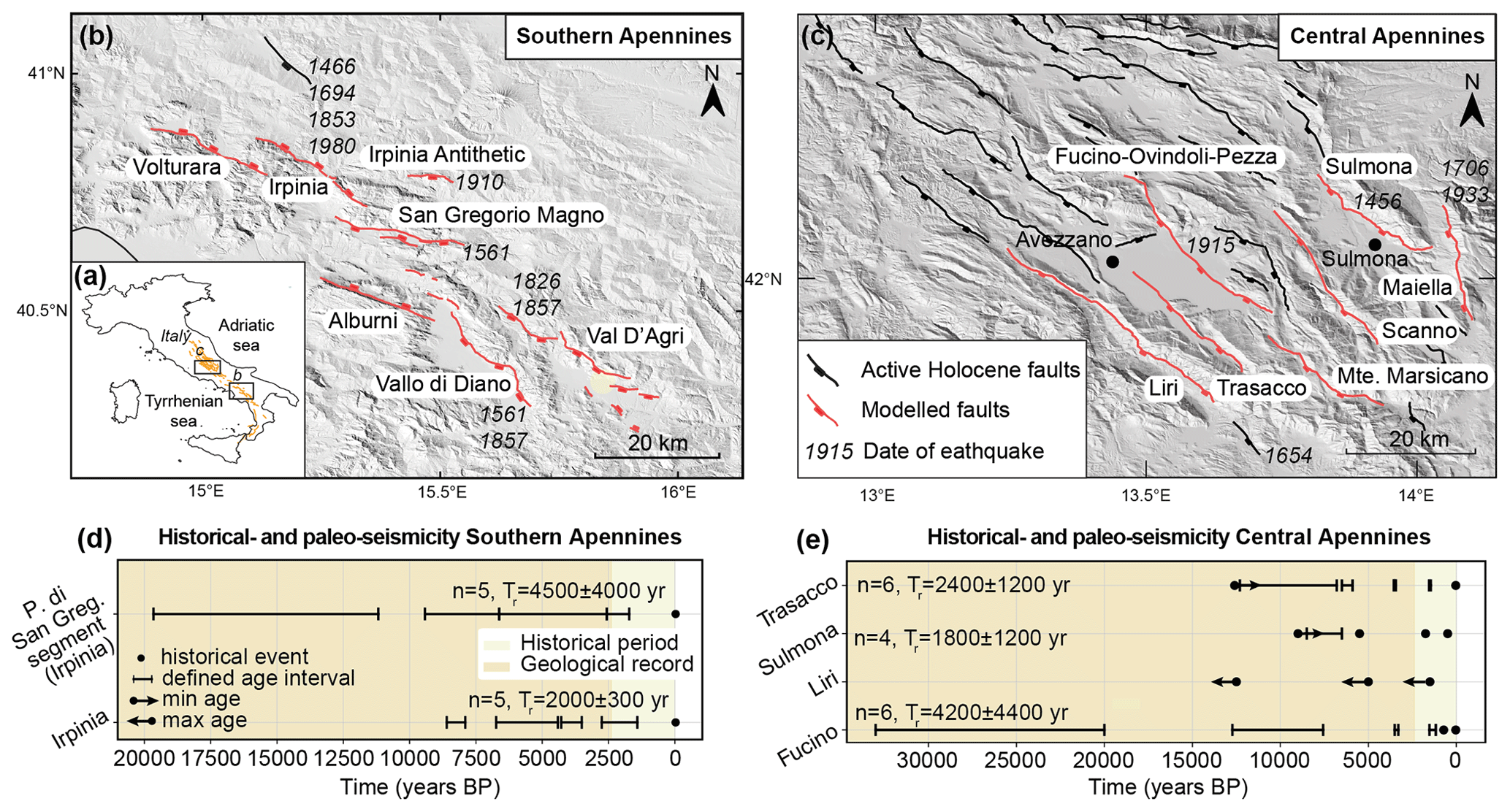
Figure 1 (a) Location of selected fault regions in Italy; (b, c) Map of the fault regions in the Apennines and historical earthquakes (post 1400  A.D.). Active Holocene fault traces in the (b) Southern Apennines (based on Sgambato et al., 2020b) and (c) Central Apennines (based on Faure Walker et al., 2021), showing the different fault network geometries between the regions, with few across-strike faults in the Southern Apennines and multiple across-strike faults for Central Apennines. Dashed black lines show the debated link between Vallo di Diano and Auletta faults and Auletta and Caggiano-Montemurro faults (see Sect. 3.1). (d, e) Chronology of paleoseismic and historical events with M > 6 in modelled faults of the (d) Southern Apennines and (e) Central Apennines (see Table B2 for details; Galadini and Galli 1999; Galli et al., 2008, 2015, 2016; Pace et al., 2020; Pantosti et al., 1993). Whisker plots represent the estimated time range of seismic events. The number of paleoseismic events per fault with defined aged brackets (n), and their estimated mean and standard deviation of recurrence time (Tr) is also shown.

A subset of faults in the Southern and Central Apennines was chosen for computational efficiency. The chosen fault networks differ in the number, length and orientation of faults. The chosen sector in the Central Apennines is characterised by a wide fault network, with up to 8 faults arranged NW-SE (Fig. 1b), whereas the Southern Apennines has a narrower fault network with fewer faults accommodating the extension, with a maximum of 3 across-strike faults (Fig. 1c). These faults are associated with moderate to large magnitude earthquakes (M_w 5.5–7; e.g,. Bagh et al., 2007; Chiaraluce et al., 2005, 2022; Guidoboni et al., 2019). In the Southern Apennines, the historical record documents 9 earthquakes of M_w > 5.6 since 1466 associated with the studied faults (Fig. 1c, Table B1; Cello et al., 2003; Galli et al., 2006, 2014; Galli and Peronace, 2014; Giardini et al., 1996; Rovida et al., 2020; Westaway, 1993; Westaway and Jackson, 1987). Two multi-fault seismic sequences have occurred in the region: one in 1857 of estimated M_w 7.1 involving either the Vallo di Diano and the Val D'Agri faults (Benedetti et al., 1998; Cello et al., 2003; Galli et al., 2006) or the Caggiano-Montemurro fault (Bello et al., 2022); and a second in 1980 of M_w 6.81 that ruptured the Irpinia (also known as Monte Marzano fault, e.g., Galli, 2020), and Irpinia antithetic faults, as well as possibly the San Gregorio fault (Sgambato et al., 2025). This rupture included a northeast dipping segment of the Irpinia fault known as the Pantano di San Gregorio segment (D'Addezio et al., 1991; Fig. 1b). The 1980 event was the largest earthquake instrumentally recorded in the Apennines (Bernard and Zollo, 1989). In the studied segment of the Central Apennines, the historical record includes 7 earthquakes of M_w > 5.6 since 1456 associated with the studied faults, including the 1915  A.D. Fucino earthquake. Paleoseismic data is available for 1 and 4 of the modelled faults in Southern and Central Apennines, respectively (Fig. 1d and e, Table B2).

3 Methods

3.1 Model set-up

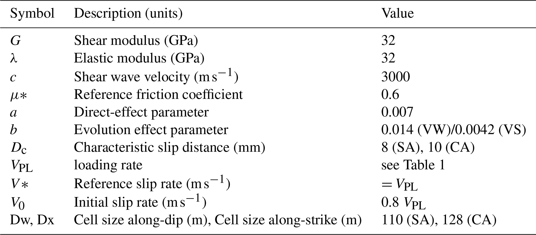
We use the boundary-element software QDYN (Luo et al., 2017) to model SEAS on the Southern and Central Apennines fault networks, each composed of 2D normal faults governed by rate-and-state friction, embedded in a 3D elastic medium (see Appendix A for a description of the governing equations).

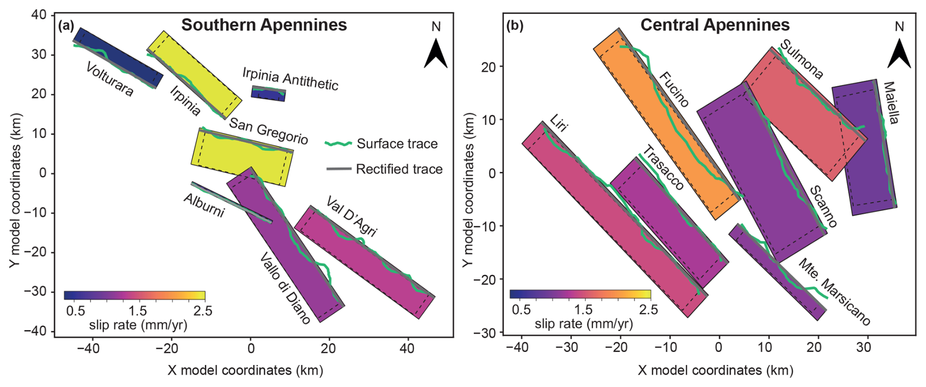
Figure 2 Map view of the model geometry for the (a) Southern Apennines and (b) Central Apennines fault network. Fault planes are colour-coded according to their Holocene slip rate. Black dashed lines show the velocity-weakening asperities. Surface fault traces (green) derived from (Faure Walker et al., 2021; Mildon et al., 2019; Sgambato et al., 2020b) and rectified traces (grey) used in the model are also shown.

Table 1 Geometry and long-term slip rate of modelled fault sources in the Southern and Central Apennines. References for slip rate: [1] (Valentini et al., 2017) [2] (Faure Walker, 2010) [3] (Galli et al., 2014) [4] (Cinque et al., 2000) [5] Fault2SHA database (Faure Walker et al., 2021) [6] (Morewood and Roberts, 2000) [7] (Roberts and Michetti, 2004) [8] (Faure Walker et al., 2019) [9] (Papanikolaou et al., 2005).

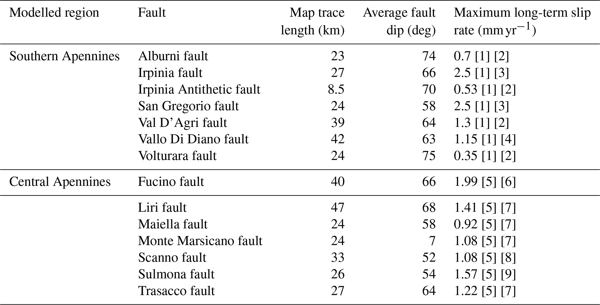
We model 7 faults in the Southern Apennines (Alburni, Irpinia, Irpinia Antithetic, San Gregorio Magno (here referred as “San Gregorio”), Val D'Agri, Vallo Di Diano and Volturara faults; Fig. 2a) and 7 faults in the Central Apennines (Fucino-Ovindoli-Pezza (here referred as “Fucino”, also known as San Benedeto dei Marsi-Goia dei Marsi segment by Galadini and Galli, 1999), Liri, Maiella, Monte Marsicano, Scanno, Sulmona (also known as Monte Morrone fault by Galli et al., 2015, and Trasacco faults; Fig. 2b). All selected faults are active, with documented Holocene throw (Faure Walker et al., 2021; Sgambato et al., 2020a; Valentini et al., 2017). In preliminary trials, we identified that the inclusion of three other active faults in the Central Apennines (Parasano-Pescina, Tremonti and San Sebastiano faults) led to unrealistically high stress concentrations in the Fucino fault, which caused numerical instability forcing the simulation to stop prematurely. For these computational reasons, we exclude the three active faults from the Central Apennines model. The potential implications of this exclusion are addressed in the Discussion section.

The trend and average dip of each fault is taken from published sources (Fault2SHA database, Faure Walker et al. (2021); Mildon et al. (2019); and Sgambato et al., 2020b) (Table 1). For the Central Apennines, we use the definition of “main fault traces” of Fault2SHA, which represent how faults segments have been interpreted to be linked at depth, at the scale recommended for input into hazard models (Faure Walker et al., 2021). For the Southern Apennines, which are not covered by the Fault2SHA database, we utilise fault traces from Sgambato et al. (2020b). The geometry and extent of some of these fault traces is debated. For instance, in some interpretations the NW segment of Vallo di Diano fault (also known as Auletta fault or Caggiano fault) is a separate segment from this fault and continues SE (Galli et al., 2006) or even joins with Val D'Agri fault as part of the Caggiano-Montemurro fault system (Bello et al., 2022) (Fig. 1b). Here, we follow the interpretation of Sgambato et al. (2020b), where the NW segment is part of Vallo di Diano fault based on the field-based evidence of the slip vector orientations (Papanikolaou and Roberts, 2007).

To accommodate QDYN current restriction to a uniform strike for each dip-slip fault, we rectify the fault traces (Fig. 2). The fault depths are set in most of the cases to 15 km, which is taken as approximately the depth of the brittle-ductile transition and is consistent with hypocentral depths observed in the region (Chiarabba et al., 2005; Chiaraluce et al., 2005; Frepoli et al., 2011). We make two exceptions for fault geometry parameters. The Irpinia Antithetic fault, being relatively short (length  < 15 km), is assigned a depth of 8 km to maintain an aspect ratio of 1 (Nicol et al., 1996). This modification has implications for the generation of full ruptures, as addressed in the Results and Discussion sections. We limited the Alburni fault to a depth of 3 km to prevent numerical instabilities caused by the intersection with the Vallo di Diano fault. This approximation may lead to an underestimation of its potential involvement in multi-fault rupture sequences and stress transfer, especially near the Vallo di Diano fault. However, the Alburni fault is not thought to have ruptured in historical times, but it is considered to have been active between late Pliocene and late Pleistocene (Gioia et al., 2011; Soliva et al., 2008).

We assign a constant loading rate value to each fault, corresponding to the maximum Holocene slip-rate (Fig. 2; Cinque et al., 2000; Faure Walker, 2010; Faure Walker et al., 2019, 2021; Galli et al., 2014; Morewood and Roberts, 2000; Papanikolaou et al., 2005; Roberts and Michetti, 2004; Valentini et al., 2017). Preliminary trials conducted in this study and from previous work (e.g., Yin, 2022), show that in the implicit LSODA solver used here (Yin et al., 2023), slip rates below 1 mm yr⁻¹ can cause velocity values to drop below numerical precision, especially when neighbouring faults also exhibit low slip rates. We suspect that this is due to the difference between the minimum and maximum slip rates present in the system, which span many orders of magnitude, causing precision underflow when jointly solving the system of equations. Therefore, we scale up the loading rate by a factor of 100 which represents the minimum value required to ensure numerical stability across the full fault network, while remaining as close as possible to the geologically inferred loading rates. Based on these trials and on previous studies (Yin, 2022) we find that this scaling has minimal impact on seismicity statistics, once we correct simulations outputs (such as recurrence times) for this upscaling factor (see Appendix B). All time scales reported hereafter account for this correction factor.

The set up does not contain further complexities such as variable fault geometry, heterogeneous slip-rate distribution along the fault strike, and or complex heterogeneous distribution of frictional properties. Although these elements may generate heterogeneous stress concentrations that might act as barriers to rupture propagation or as regions of earthquake nucleation (Delogkos et al., 2023; Hillers et al., 2007; Luo and Ampuero, 2018; Mildon et al., 2019; Rodriguez Piceda et al., 2025b), we chose to omit these complexities to primarily focus on the impact of fault network geometry and fault stress interactions on rupture dynamics.

The simulations run for 11 kyrs to ensure a sufficient number of seismic events for statistical analysis, with the first 500 years discarded as the spin-up phase. To compute the duration of a seismic event, we consider that it starts when one fault element has a slip rate larger than 0.1 m s⁻¹ and stops when the slip rate of all the elements slip drops below 0.01 m s⁻¹.

We additionally simulate SEAS on each individual isolated fault included in the Southern and Central Apennines networks to determine their reference behaviour in the absence of stress interactions with other faults. These simulations use the same parametrization as the full fault network simulations described above.

3.2 Fault network and seismic cycle characteristics

To quantify the effect of across-strike faults, we compute an across-strike interaction index (AI) for each fault i as:

$$\begin{array}{}\text{(1)}& {\text{AI}}_i={\sum }_{j\ne i}{\displaystyle \frac{\mathrm{1}}{s_{ij}}}\end{array}$$

where j are the indices of other across-strike faults, s_ij is the across-strike separation between fault i and fault j (see Appendix C for a detailed definition of the separation between faults). The inverse weighting $\frac{\mathrm{1}}{s_{ij}}$ ensures that faults that are closer contribute more to the index than those farther away. Faults with a larger number of across-strike interactions have a higher across-strike interaction index. We focus on across-strike density since previous work (Rodriguez Piceda et al., 2025b) showed that across-strike interactions dominate over along-strike interactions at comparable distances.

To characterise the complexity of seismic cycles, we compute three metrics: the coefficient of variation of recurrence times of individual faults (CV_Tr), the normalised number of partial ruptures ($N_{\mathrm{p}}^{\prime }$) and the coefficient of variation of rupture lengths (${\text{CV}}_{\text{RL}}^{\prime }$).

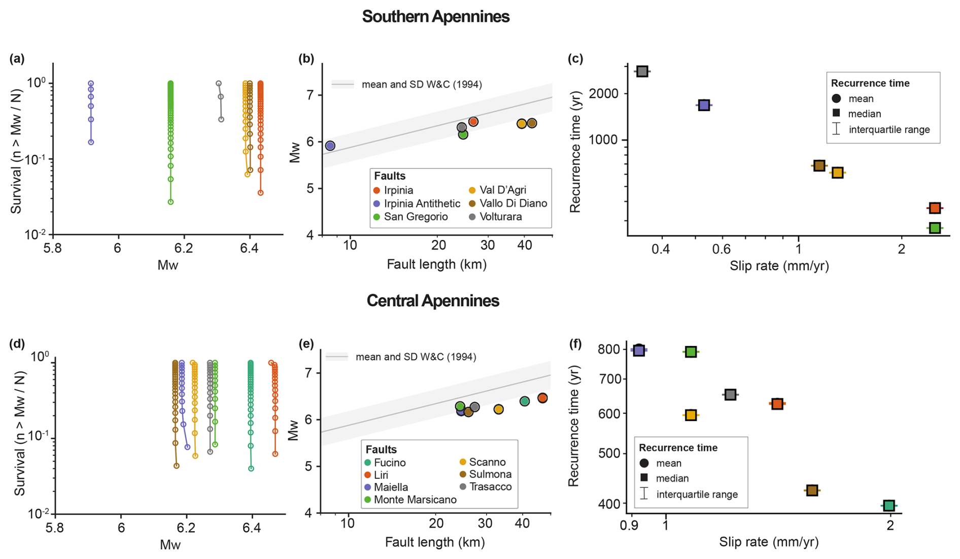
Figure 3 Earthquake cycle simulations of isolated faults in the (a–c) Southern and (d–f) Central Apennines. (a, d) Magnitude-frequency distributions of earthquakes on each fault (shown as survival functions: number of events with a M_w larger than a given value, normalised by the total number of events). Their near vertical appearance indicates all isolated faults in this model have characteristic-earthquake behaviour, with very narrow range of M_w. (b, e) Comparison between modelled seismic events and mean and standard deviation of empirical relationships of subsurface rupture length vs. M_w (Wells and Coppersmith, 1994); (c, f) Mean, median and interquartile range of earthquake recurrence times vs. long-term tectonic slip rate of individual faults. Note how the mean and median are equal, and the interquartile range is below the marker size for all faults across both regions.

CV_Tr is calculated as:

$$\begin{array}{}\text{(2)}& {\text{CV}}_{\mathrm{Tr}}={\displaystyle \frac{\text{std}\left(\mathrm{Tr}\right)}{\text{mean}\left(\mathrm{Tr}\right)}}\end{array}$$

where Tr is the distribution of time intervals between consecutive events on the same fault. CV_Tr=0 indicates strictly periodic seismic cycles; 0 < CV_Tr < 0.5, strongly periodic; $\mathrm{0.5}\le {\text{CV}}_{\mathrm{Tr}}\le \mathrm{1}$, weakly periodic; CV_Tr=1 indicates that event timing is random and independent of other events; and CV_Tr > 1 implies event clustering (Boschi et al., 1995).

$N_{\mathrm{p}}^{\prime }$ is calculated as:

$$\begin{array}{}\text{(3)}& N_{\mathrm{p}}^{\prime }={\displaystyle \frac{N_{\mathrm{p}}}{N}}\sqrt{{\displaystyle \frac{L_{\mathrm{\infty }}}{W_{\mathrm{s}}}}}\end{array}$$

where N_p is the number of partial ruptures, N the total number of events for each fault, W_s the seismogenic width and L_∞ the nucleation length (Eq. A5) introduced by Rubin and Ampuero (2005).

${\text{CV}}_{\text{RL}}^{\prime }$ is calculated as:

$$\begin{array}{}\text{(4)}& {\text{CV}}_{\text{RL}}^{\prime }={\displaystyle \frac{\left(\text{std}\right(\text{RL})/\text{mean}(\text{RL}\left)\right)}{(W_{\mathrm{s}}/L_{\mathrm{\infty }})}}\end{array}$$

where RL is the distribution of rupture lengths.

Both $N_{\mathrm{p}}^{\prime }$ and ${\text{CV}}_{\text{RL}}^{\prime }$ are normalised by $W_{\mathrm{s}}/L_{\mathrm{\infty }}$ to account for fault-to-fault differences in seismogenic width W_s and the nucleation length L_∞, enabling comparison of partial ruptures and rupture length variability (Cattania, 2019; Barbot, 2019). Overall, faults with larger CV_Tr, $N_{\mathrm{p}}^{\prime }$, ${\text{CV}}_{\text{RL}}^{\prime }$ have seismic cycles characterised by less periodic recurrence, more frequent partial ruptures and a wider range of rupture sizes.

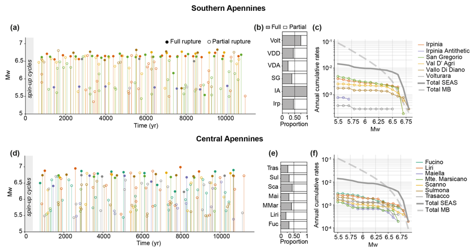
Figure 4 Earthquake statistics from the model results for the Southern (a–c) and Central (d–f) Apennines fault networks. Time distribution of simulated full- and partial-rupture events with stems and markers colour-coded by fault in the (a) Southern Apennines and (d) Central Apennines. Earthquakes in the first 5 years correspond to spin-up phases, thus are not included in the analysis. (b, e) Proportion of full and partial ruptures relative to the total number of events per fault in the (b) Southern Apennines and (e) Central Apennines. (c, f) Magnitude–frequency distributions of seismic events expressed as annual cumulative rates (number of annual occurrences with M_w greater than a given value) for individual faults in the (c) Southern Apennines and (f) Central Apennines. Annual cumulative rates for the entire fault network derived from the SEAS models, together with estimates obtained using the moment-budget method (MB; Appendix H), are also shown. Colour legend for each fault is shown in panels (c) and (f).

4 Results

4.1 Seismic cycles on isolated faults

In all single-fault simulations, faults rupture with a characteristic magnitude M_w (Fig. 3a and d), which is linearly related to the logarithm of fault length (Fig. 3b and e). In the Southern Apennines, M_w on individual faults ranges from 5.9 for the Irpinia Antithetic fault to 6.4 for the Irpinia and Vallo di Diano faults (Fig. 3a). In the Central Apennines, M_w values range from 6.2 on the Sulmona fault to 6.5 on the Liri fault (Fig. 3d). Notably, most earthquakes in both fault networks have magnitudes smaller than those predicted by empirical relationships of subsurface rupture length vs. magnitude (Fig. 3b and e; Wells and Coppersmith, 1994).

The resulting seismic cycles are periodic, with recurrence intervals inversely correlated to the prescribed long-term slip rate (Fig. 3c and f). Mean recurrence times range from 300 years in San Gregorio fault to ∼ 1700 years in Volturara fault in the Southern Apennines (Fig. 3c); and from 400 years in Fucino fault to 800 years in Maiella fault in the Central Apennines (Fig. 3f).

4.2 Seismic cycles on fault networks

We generated two synthetic seismic catalogues for the interacting fault networks, containing 150 events in the Southern Apennines and 154 events in Central Apennines (Fig. 4a and d). The magnitude range produced by faults within the networks is broader than that of isolated faults: from M_w 5.3 to 6.8 in the Southern Apennines (Fig. 4c) and from M_w 5.3 to 7 in the Central Apennines (Fig. 4f), broadly matching observed earthquake magnitudes. In our Southern Apennines model, the Alburni fault does not produce any earthquakes. This is likely due to its shallow seismogenic zone (down to a depth of 2.65 km). Unlike the isolated fault models, not all ruptures extended for the whole length of the faults, with some ruptures terminating as partial ruptures. Most faults generate both full and partial ruptures, with a larger proportion of partial ruptures (Fig. 4b and e). Due to the generation of full and partial ruptures, the magnitude-frequency distributions show a truncated Gutenberg-Richter distribution (Stirling et al., 1996). The largest magnitude events are limited by the length of the longest fault, in our case, the Vallo di Diano fault in Southern Apennines (Fig. 4c) and the Liri fault in Central Apennines (Fig. 4f). The Irpinia Antithetic fault is the only fault to consistently generate full ruptures with a characteristic M_w of 5.8. This is likely due to its small fault dimensions (8 km in length and depth), which limits its potential for partial ruptures in the model (Barbot, 2019; Cattania, 2019; Cattania and Segall, 2019) (Fig. 4b and c).

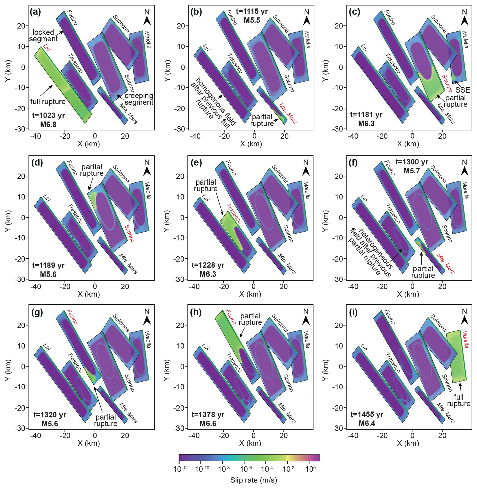
Figure 5 Map view of slip-rate snapshots showing the final timestep of the coseismic phase for each event in a subset of modelled ruptures in the Central Apennines including full ruptures, partial ruptures and slow slip events (SSE). Monte Marsicano fault is abbreviated as Mte. Mars.

To highlight the rupture styles observed in our simulation, Fig. 5 shows a subset of events that occur in the Central Apennines between two full ruptures, one on the Liri fault and one on the Maiella fault. While a full rupture occurs on one fault, the remaining faults stay locked (Fig. 5a). The full rupture affects both the locked and surrounding creeping segment of the fault (Fig. 5a), and it is followed by partial ruptures in the remaining faults (Fig. 5b–h). Some of these partial ruptures occur consecutively on the same fault (e.g. Fucino fault, Fig. 5g and h), with some separated by hours (e.g. two events on the Vallo di Diano fault at 5450 year and two events on the Monte Marsicano fault at 8360 year, not shown in Fig. 5, Videos S2 and S3; Rodriguez Piceda et al., 2026). Subsequent events in this type of sequence commonly rupture the fault segments that were not involved in the prior earthquake. Simulated full and partial ruptures nucleate typically at the base of the locked seismogenic zone (Videos S2 and S3; Rodriguez Piceda et al., 2026). Overall, while full-rupture events homogenise the slip rate field in locked fault patches (Fig. 5b), partial ruptures introduce a heterogeneous slip rate field in these patches (Fig. 5f), a direct consequence of the stress concentration left behind by the arrested partial ruptures. The heterogeneous slip rate then influences the nucleation and propagation of subsequent events (Video S2; Rodriguez Piceda et al., 2026), acting either as nucleation sites or barriers where ruptures terminate. In addition to the observed earthquakes, aseismic slip in the form of slow slip events sometimes occurs simultaneously with seismic events on other faults (Fig. 5c, Video S2; Rodriguez Piceda et al., 2026). The occurrence of full and partial ruptures, as well as slow-slip events, shows the more diverse slip behaviour of faults within a network compared to the isolated fault models.

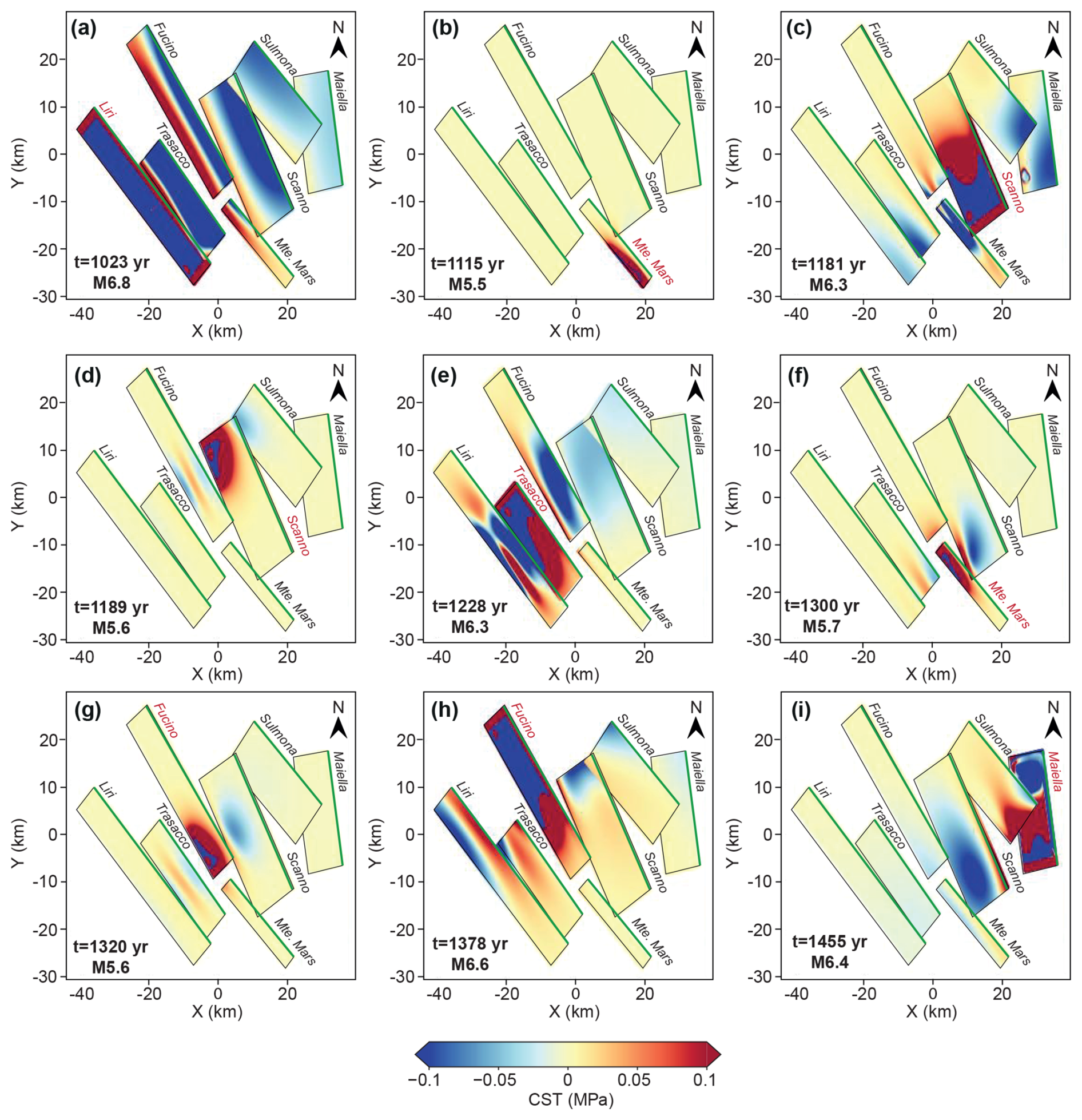
Figure 6 Coseismic Coulomb Stress Transfer (CST) for a subset of modelled earthquakes in the Central Apennines shown in Fig. 5, with fault planes projected to a horizontal surface.

To illustrate the stress changes introduced by each seismic event we computed the coseismic Coulomb stress transfer (CST) for each seismic event as (King et al., 1994):

$$\begin{array}{}\text{(5)}& \mathrm{\Delta }C=\mathrm{\Delta }\mathit{\tau }-\mathit{\mu }(\mathit{\theta },V)\mathrm{\Delta }\mathit{\sigma }\end{array}$$

where Δτ is the shear stress-change, Δσ is the normal stress change before and after the earthquake and μ(θ,V) the rate-and-state friction coefficient at the receiver fault location. Figure 6 shows the CST for the same subset of modelled ruptures as in Fig. 5, and the CST evolution from all events in both fault network models are shown in Figs. E1 and E2. Most full and partial ruptures introduce a heterogeneous stress change on nearby faults, due to the range of fault strike and partial overlaps between faults in the network (Fig. 6). In the rare cases where faults are almost parallel and with a near 100 % overlapping area, a full-rupture event on one fault introduces a homogenous stress change. This can be observed for the Liri and Trasacco faults, where a full-rupture event on Liri fault negatively loads Trasacco fault (Fig. 6a).

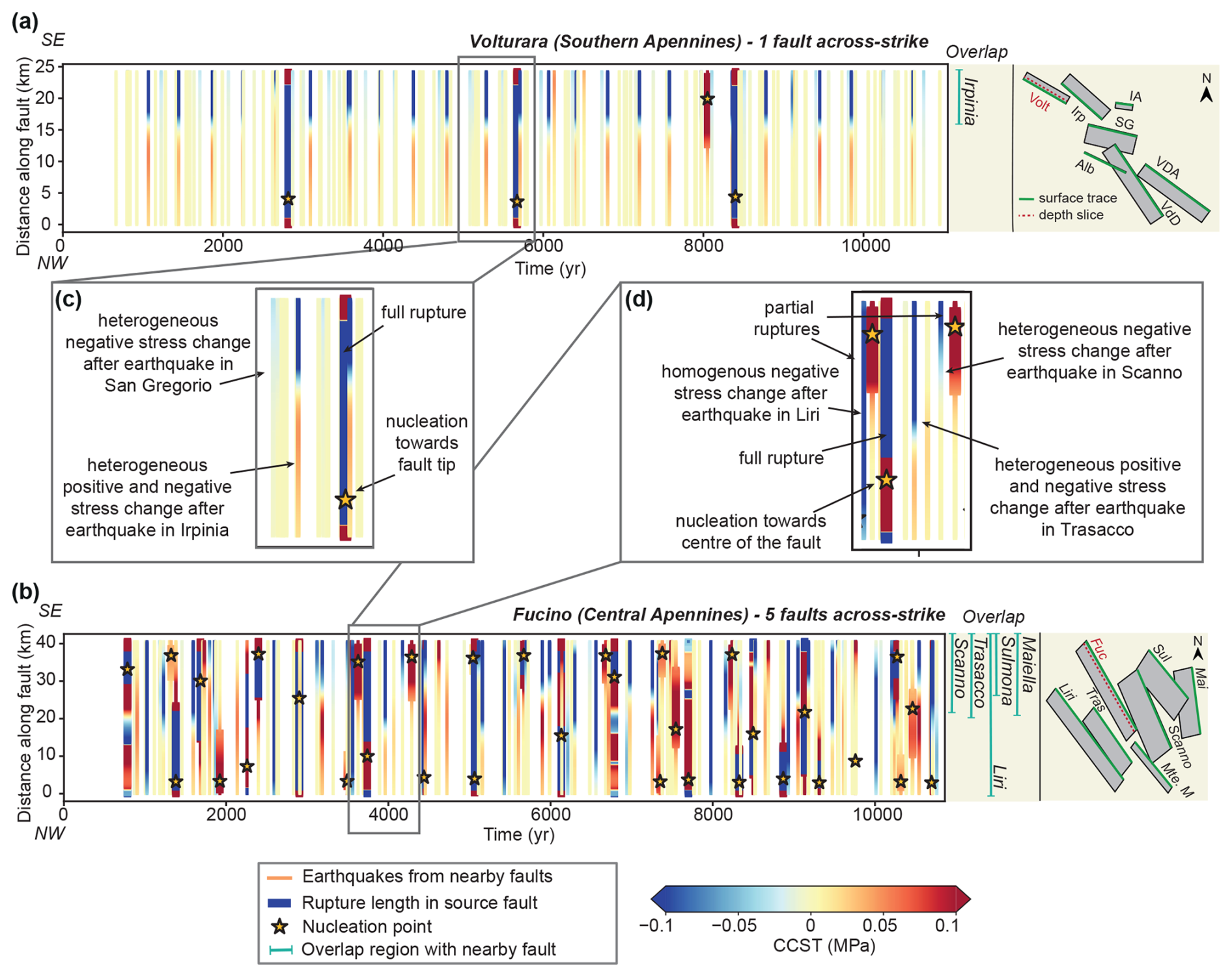
Figure 7 (a) Coseismic Coulomb stress transfer (CST) on the Volturara fault, which has 1 across-strike fault that overlaps; (b) CST on the Fucino fault, which has 5 neighbouring across-strike faults that overlap. Coloured backgrounds show the stress changes following each event along a depth slice close to the top of the velocity weakening asperity (location example shown in right panels of Fig. 7a and b). Coseismic CST due to ruptures on the fault are indicated by the thick vertical slices that coincide with a star (nucleation point on the fault); thin vertical slices without corresponding star represent the coseismic CST due to ruptures on neighbouring faults. On the right side of panels (a) and (b) we indicate the fault segments that are overlapping with neighbouring faults (taken as the maximum length measured along-strike from the NW fault tip, see Fig. D2, Appendix D), including an inset with map view of fault surfaces. (c) and (d) are zoom-ins highlighting contrasting behaviours between the faults. The Volturara fault shows spatially homogeneous stress changes and simple seismic cycles, with full ruptures and nucleation near fault tips. The Fucino fault exhibits spatially complex coseismic CST patterns, partial ruptures, and nucleation that is more distributed across the fault. Faults with limited across-strike interaction tend to show simpler rupture behaviour, while those with multiple across-strike interactions show a more heterogeneous stress evolution and complex earthquake cycle.

Figure 7a and b shows the evolution of CST and nucleation point of each event along a depth slice near the top of the velocity-weakening asperities (∼ 1700 m) of the Volturara and Fucino faults, compared to the extent of overlap with adjacent faults in the fault network (Figs. E3 and E4 show the same but for the remaining faults). Faults such as Volturara, which have few nearby, partially overlapping, across-strike faults, tend to show coseismic stress changes that remains broadly similar through successive earthquake cycles. Seismicity comprises mainly full ruptures that nucleate near fault tips (Fig. 7a and c). These nucleation locations correspond to regions of elevated stressing rates produced by the backslip loading method, which remain highest near fault tips despite the inclusion of velocity-strengthening buffer regions (Appendix A).

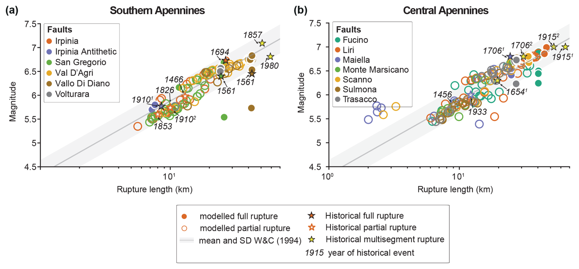
Figure 8 Comparison between modelled seismic events, historical ruptures and empirical relationships of subsurface rupture length vs. Magnitude (Wells and Coppersmith; 1994) for (a) Southern Apennines and (b) Central Apennines. Magnitude refers to M_w for SEAS simulations and empirical scaling relationships; magnitudes of historical earthquakes are defined in Table B1 (Appendix B). Modelled and historical single-fault events are colour-coded according to the source fault. Superindices on dates of historical events refer to alternative scenarios. 1910¹: scenario with rupture of entire Irpinia antithetic (Galli and Peronace, 2014); 1910²: scenario with 10 km rupture of Irpinia fault (Galli and Peronace, 2014); 1654¹: scenario with 13 km rupture of Southern section of Liri and entire Fibreno faults (outside of study area; (Guidoboni et al., 2019); 1706¹: scenario with rupture of entire Maiella fault (Guidoboni et al., 2019); 1706²: scenario with rupture of entire Maiella and Palena faults (outside of study area; (Guidoboni et al., 2019); 1915¹ scenario with rupture of entire Fucino, Parasano and San Sebastiano faults (Michetti et al., 1996); 1915² scenario with rupture of entire Fucino, Luco and Trasacco faults (Michetti et al., 1996) (see Table B1, Appendix B).

Conversely, faults with multiple neighbouring across-strike faults, such as Fucino fault (Fig. 7b and d), show a more spatially heterogeneous stress evolution and complex earthquake cycles consisting of full and partial ruptures. Additionally, the nucleation of full and partial ruptures is not necessarily confined to fault tips. Instead, partial ruptures that are either isolated or the first in a sequence often occur in areas where faults overlap. Therefore, the number and arrangement of across-strike faults, and the heterogeneous coseismic stress changes they induce, have a strong control on the earthquake cycle of individual faults.

We compared the magnitudes and rupture lengths of the modelled events with historical seismicity (Table B1, Appendix B) and empirical relationships between magnitude and subsurface rupture length (Wells and Coppersmith, 1994; Fig. 8a and b). Our models are able to reproduce the magnitude and rupture length of the historical single-fault events, including the two proposed scenarios for the 1910 earthquakes in Southern Apennines (Galli and Peronace, 2014). However, we are unable to reproduce multi-fault events as recorded in the historical seismicity catalogue (e.g. the 1857 and the 1980 seismic sequences in the Southern Apennines; one of the proposed scenarios for the 1706 sequence and the 1915 sequence in the Central Apennines; Table B1, Appendix B). Compared to the empirical relationships of magnitude vs. subsurface length, most of our modelled events (99 % in Southern Apennines and 92 % in Central Apennines) fall within the range marked by the mean and standard deviation of Wells and Coppersmith (1994).

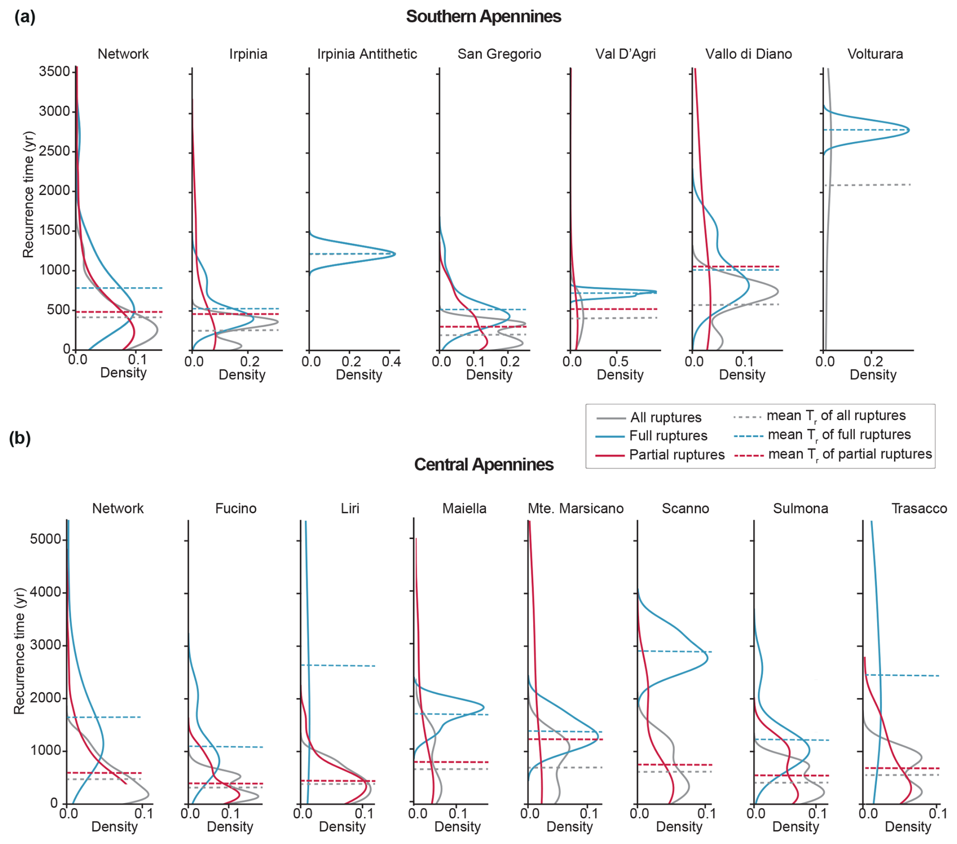
Figure 9 Variation of recurrence time (Tr) for the (a) Southern and (b) Central Apennines, shown as kernel density plots (KDE) and mean recurrence time, for the entire fault network and for individual faults considering the “All-ruptures”, “Full-ruptures” and “Partial-ruptures” catalogues. Volturara fault produced only 1 partial rupture, thus no KDE for its partial-rupture catalogue could be computed. As this single partial rupture is included in the “All-ruptures” catalog but absent from the “Full-rupture” catalog, the two distributions are different. Note how the density scale varies by fault, and that partial ruptures typically display a greater range in recurrence time than full ruptures.

Recurrence times vary between the two modelled regions, and depend on whether the full catalogue is considered, or whether it is split between full and partial ruptures. Full catalogue recurrence times for the system and for individual faults are positively skewed, with some faults showing bi-modal distributions (Fig. 9). When the Southern and Central Apennines are compared, greater variability is observed in the mean recurrence times of the Southern Apennines, which range from 250 (San Gregorio fault) to 2100 (Volturara fault) years in the Southern Apennines compared to 300 (Fucino fault) and 700 (Monte Marsicano fault) years in the Central Apennines (Fig. 9).

Where full and partial rupture catalogues are compared, partial ruptures tend to have shorter recurrence times than full ruptures (Fig. 9a and b). Across both regions, recurrence time distributions of partial ruptures in individual faults and the system are positively skewed, spanning a wide range, from hours to years. In contrast, the recurrence time distributions of full ruptures are narrower, typically following a bimodal or normal distribution (Fig. 9).

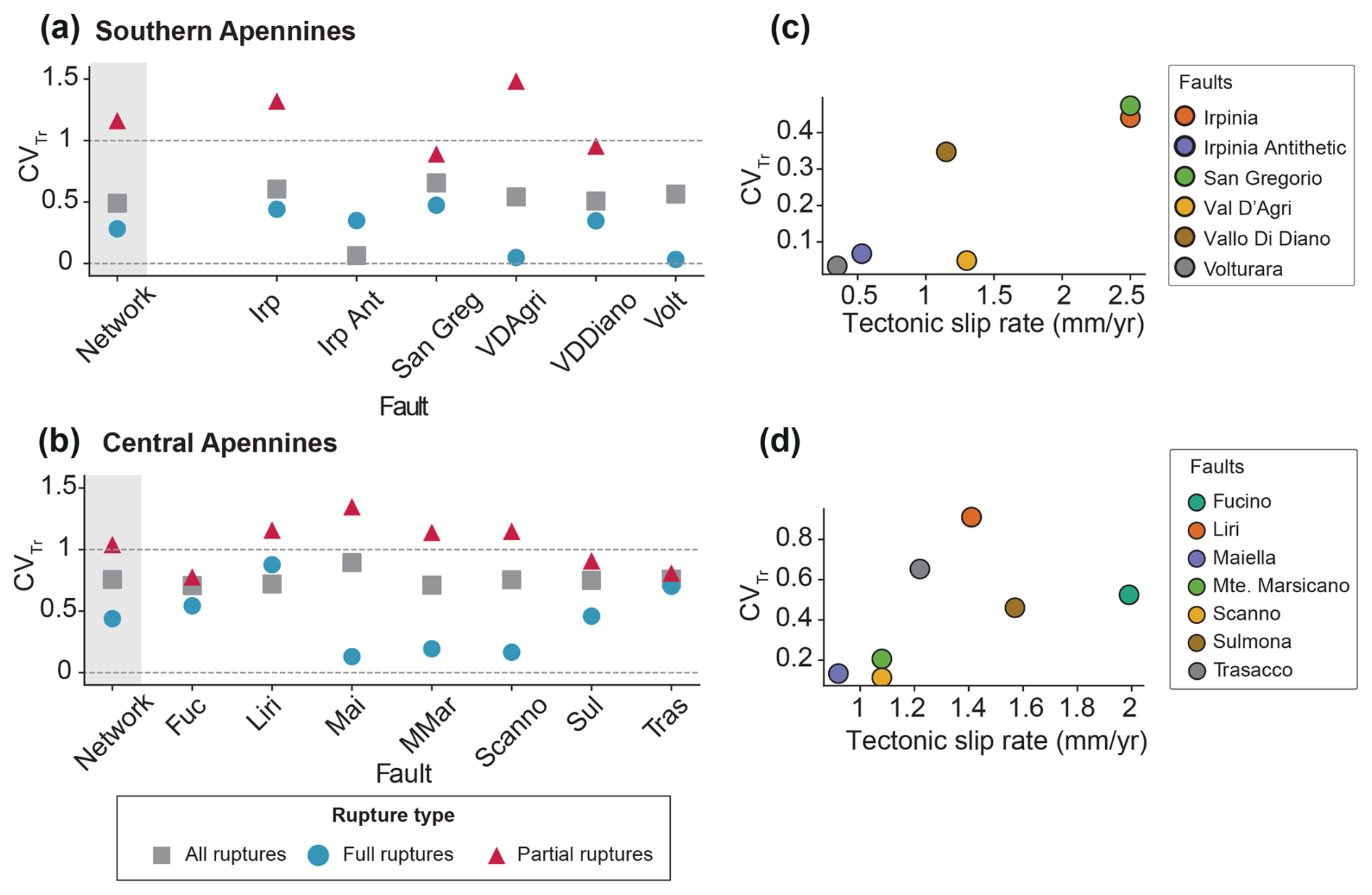
Figure 10 (a, b) Coefficient of variation of recurrence times CV_Tr of seismic events (all events, full ruptures and partial ruptures) for individual faults and entire fault network in the (a) Southern Apennines and (b) Central Apennines. Horizontal dashed lines mark the CV_Tr values of perfectly periodic (CV_Tr=0) and lower limit of random (CV_Tr=1) seismic cycles. (c, d) Long-term slip rate vs. CV_Tr of all events for the (c) Southern Apennines and the (d) Central Apennines. Seismic cycles of full-rupture events are either strongly or weakly periodic, while cycles of partial ruptures are weakly periodic, random or clustered. The fault network in the Central Apennines has less periodic seismic cycles than in the Southern Apennines.

The catalogue periodicity is assessed though the coefficient of variation of recurrence time CV_Tr. For the all-rupture catalogues, both regions display weakly periodic behaviour (CV_Tr = 0.5–1, Fig. 10a and b). The exception is the Irpinia Antithetic fault, which maintains a more periodic recurrence (Fig. 10a). Overall, the Central Apennines exhibits less periodic seismic cycles (CV_Tr=0.8, Fig. 10b) compared to the Southern Apennines (CV_Tr=0.5, Fig. 10a).

Periodicity differs between full and partial ruptures as well as between regions. Faults generate full rupture events with varying degrees of periodicity. In the Southern Apennines (Fig. 10a), all faults show strongly periodic full-rupture cycles (CV_Tr < 0.5). In the Central Apennines (Fig. 10b), the behaviour is more variable: the Maiella, Monte Marsicano and Scanno faults show strongly periodic full-rupture cycles whereas the Trasacco, Liri, Sulmona and Fucino faults are weakly periodic (0.5 ≤CV_Tr < 1). Partial ruptures in both networks show less periodic behaviour than full ruptures (Fig. 10a and b). Their recurrence ranges from weakly periodic (0.5 ≤CV_Tr < 1; e.g., San Gregorio, Fucino, Sulmona and Trasacco faults) to random (CV_Tr=1, e.g., Vallo di Diano fault) or clustered (1 < CV_Tr < 1.5, e.g., Irpinia, Val D'Agri, Liri, Maiella, Monte Marsicano and Scanno faults). CV_Tr of full-rupture events tends to increase with increasing long-term slip rate (Fig. 10c and d).

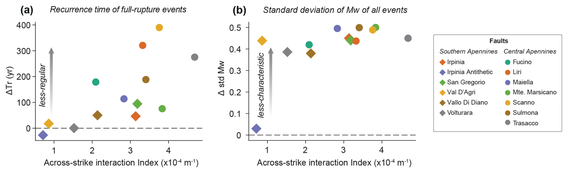
Figure 11 Comparison of earthquake cycles between single-fault simulations and fault-network simulations in terms of event (a) recurrence time (Tr) of full-rupture events (ΔTr = mean Tr_network − $\text{mean }{\mathrm{Tr}}_{\text{single}})/\text{mean }{\mathrm{Tr}}_{\text{single}}$ and (b) standard deviation of magnitude of full-rupture events (ΔstdM_w = $\text{std}{M_{\mathrm{w}}}_{\text{network}}-\text{std}{M_{\mathrm{w}}}_{\text{single}}$) as a function of the across-strike interaction index (Eq. 1). ΔT_r=0 indicates regular recurrence, while positive (negative) values correspond to longer (shorter) recurrence times in the fault-network simulations relative to the single-fault simulations. ΔstdM_w=0 indicates characteristic magnitude distribution, while increasingly positive values indicate broader magnitude-frequency distributions in the fault-network simulations. Faults with multiple faults across-strike (larger AI) show larger differences in recurrence time and standard deviations of magnitude compared to single-fault simulations, indicating a greater deviation from their characteristic periodic behaviour.

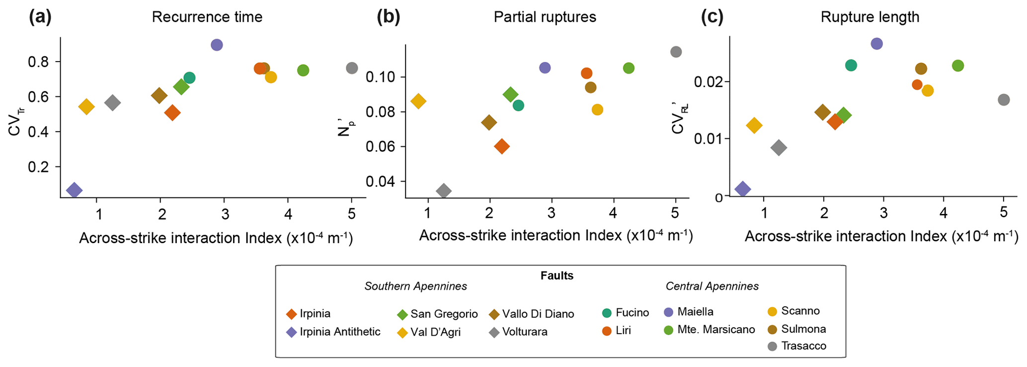
Figure 12 Relationships between fault network geometry, described by the across-strike interaction index (AI), and (a) coefficient of variation of recurrence times (CV_Tr), (b) number of partial ruptures ($N_{\mathrm{p}}^{\prime }$) and coefficient of variation of rupture lengths (${\text{CV}}_{\text{RL}}^{\prime }$) for faults in the Southern and Central Apennines. AI is calculated at a depth of 7.5 km, approximately the middle fault depth. Plots corresponding to depths of 0 and 15 km are shown in Fig. F1 (Appendix F).

4.3 Relationships between seismic cycle characteristics and fault network geometry

In the Southern Apennines, where the fault network has fewer across-strike faults and larger distances between them, the across-strike interaction index (AI) is less than in the Central Apennines, which has multiple closely-spaced across-strike faults, resulting in a higher AI due to both fault number and proximity. Fault interactions via stress transfer affect recurrence intervals and magnitudes of full-rupture events, compared to the isolated fault case (Fig. 11). Most faults produce full ruptures with longer recurrence times and larger magnitudes compared to the reference cycles on isolated fault (Fig. 11). These differences become more pronounced with an increase in the number of nearby across-strike faults in the Central Apennines, as opposed to the Southern Apennines.

Differences in earthquake cycle properties between the Southern and Central Apennines are influenced by fault network geometry (Fig. 12). When considering both networks together, we observe consistent positive correlations between the across-strike interaction index AI and the three metrics of seismic complexity (CV_Tr, $N_{\mathrm{p}}^{\prime }$, and ${\text{CV}}_{\text{RL}}^{\prime }$) with mean Spearman values ranging from 0.55 to 0.84 (Table F1, Appendix F). When analysed separately, the Southern Apennines show strong correlations for CV_Tr and ${\text{CV}}_{\text{RL}}^{\prime }$at some depths (Table F1), but no consistent trend for $N_{\mathrm{p}}^{\prime }$. In contrast the Central Apennines show weak or no correlations for all metrics (Table F1). This suggest that the geometric effects become clearer when sampling a broader range of network configurations across both regions.

5 Discussion

5.1 Comparison between simulated and natural seismic cycles in Italy

Italy's exceptional historical and paleoseismic record (D'Addezio et al., 1991; Galadini and Galli, 1996, 1999; Galli et al., 2006, 2008, 2016, 2014; Galli and Peronace, 2014; Pace et al., 2020; Pantosti et al., 1993) provides a valuable basis for evaluating our models. Our simulations are, to our knowledge, the first 3D continuum earthquake cycle models to combine rate-and-state friction with fault interactions across more than three faults, resolving nucleation and rupture self-consistently.

To compare with natural data, we focused on M ≥ 6.5 events and recurrence intervals from paleoseismic trenching (Table B2; Pace et al., 2016). After scaling due the high slip rates used in our models, natural recurrence intervals are 1.3–9.4× longer than simulated ones, consistent with our use of maximum along-strike long-term slip rates, which likely overestimate loading and shorten cycles. We expect that incorporating realistic tapered profiles would bring simulated intervals closer to observations (Delogkos et al., 2023; Faure Walker et al., 2019).

Paleoseismic recurrence times show greater variability than our nearly periodic modelled seismic cycles for full ruptures. This may reflect incomplete long-term records (e.g., Lombardi et al., 2025; Mouslopoulou et al., 2025), temporal changes in slip rates documented by cosmogenic dating (Benedetti et al., 2013; Cowie et al., 2017; Mildon et al., 2022; Roberts et al., 2024, 2025; Sgambato et al., 2025), the greater geometrical complexity of natural faults, and possibly also a larger ratio $W_{\mathrm{s}}/L_{\mathrm{\infty }}$ (Barbot, 2019; Cattania, 2019), all of which could enhance stress heterogeneity and variability.

While our models reproduce the magnitude range of historical single-fault events, they do not produce multi-fault ruptures as documented in the historical catalogue in the region (Benedetti et al., 1998; Cello et al., 2003; Galli et al., 2006). This likely stems from the quasidynamic approximation, which does not simulate dynamic triggering by seismic waves and limits stress drops, slip velocities and rupture jumping compared to fully-dynamic simulations (Thomas et al., 2014). However, studies using other quasidynamic simulators (e.g. RSQSim, (Dieterich and Richards-Dinger, 2010) have reported multi-fault rupture scenarios (Herrero-Barbero et al., 2021; Milner et al., 2021; Shaw et al., 2025). In these models, faults are more closely spaced and subject to higher effective normal stresses than our QDYN simulations (∼ 100 MPa), which increases rupture energy favouring multi-fault ruptures. In addition, model approximations of RSQSim, such as discrete state transitions and prescribed slip rates during the sliding stage (Shaw et al., 2025) might also promote larger ruptures. In comparison, our simulations resolve continuous rate-and-state friction, and include velocity strengthening barriers at fault tips and lower effective normal stress, all of which would favour rupture arrest at the fault boundaries. This limitation likely leads to an underestimation of the largest seismic events and biases the upper tail of the magnitude-frequency distribution toward single-fault ruptures. While non-periodic multi-fault ruptures would likely increase the recurrence variability and cycle complexity of individual faults, it is not expected to change the first-order role of fault network geometry identified here. Multi-fault ruptures could be promoted by stronger velocity weakening asperities or higher normal stresses, but such parameter choices would increase the computational cost, limiting their feasibility in these regional-scale simulations. A second alternative to address this would be using simulated cycles as initial conditions for fully dynamic rupture models (Galvez et al., 2020).

Despite these limitations, our results show that SEAS models can capture key behaviours of complex fault networks and generate synthetic earthquake catalogues that are directly comparable with paleoseismic data. This provides a strong basis for future simulations integrating more geologically realistic features, such as along-strike variations of slip rate and strike.

5.2 Effect of stress redistribution within a fault network on simulated seismic sequences

Our simulations show that earthquakes on networks with multiple across-strike faults, such as those in the Central Apennines, generate spatially heterogeneous stress perturbations on nearby faults. These interactions promote more partial ruptures, greater variability in rupture lengths, magnitude and nucleation locations, and less periodic behaviour of large earthquakes. In contrast, faults within more along-strike networks, like in the Southern Apennines, experience more uniform stress loading and tend to produce more periodic and characteristic seismic cycles, behaviours more similar to simulations of isolated faults (Figs. 4a, 11, and 12). These results build upon prior numerical modelling work of (Rodriguez Piceda et al., 2025b), which showed that complex and non-periodic seismic cycles emerge in a system of two across-strike normal faults. They also extend prior CST modelling work (Sgambato et al., 2020b, 2023), which showed that relatively isolated faults experience more regular stress loading histories dependent on interseismic loading than networks with multiple faults arranged across-strike.

The effects of fault network geometry can be isolated when other factors such as long-term slip rate are considered constant. A clear example of the influence of fault network geometry comes from the Central Apennines, where the Scanno and Monte Marsicano faults have similar slip rates (Table 1), yet they have contrasting seismic cycle characteristics. The Monte Marsicano fault exhibits more irregular rupture timing, partial ruptures and rupture extent variability than the Scanno fault (Fig. 12), likely due to the influence of multiple closely-spaced CST sources (Maiella, Sulmona, Scanno and Trasacco, Figs. E2e, f and E4, Appendix E), and therefore higher across-strike interaction index.

Fault networks also show longer recurrence times and larger magnitudes of full-rupture events, than the same faults modelled in isolation (Fig. 11). This results from stress interactions delaying full ruptures, allowing more time for fault healing and strength recovery, which leads to larger stress drops and higher seismic moments. Consequently, the magnitude versus rupture length scaling for fault networks (Fig. 8) better matches natural variability (Wells and Coppersmith, 1994), indicating that stress interaction among faults may contribute to the scatter seen in empirical scaling relationships.

Although not included in the simulations, the Parasano-Pescina, Tremonti and San Sebastiano may influence the seismic sequences of the Central Apennines fault network. Due to their limited area, the Parasano-Pescina and Tremonti faults would likely produce full-rupture events, similar to the Irpinia Antithetic fault in the Southern Apennines (Fig. 4a–c). The inclusion of these tree faults would increase the number of across-strike interacting fault segments, thus promoting more stress heterogeneities in neighbouring faults such as Fucino, Scanno and Trasacco, and potentially leading to more complex seismic cycles or multi-fault ruptures. Given the limitations of the modelling framework, it is currently not feasible to investigate these interactions within a network-wide approach

Our focus is on normal fault networks, thus a remaining question is whether the findings will be applicable to strike-slip and thrust faults. We speculate that similar effects could occur in these settings, with the outcome depending on the degree of development of the fault network. Fault networks in late stage of development tend to evolve into more localized structures, reducing the fault overlap and the extent of interactions. In contrast, interaction effects may be more pronounced in early-stage networks, where a higher number of closely spaced overlapping faults are more common.

5.3 Role of long-term slip rate in stress interaction effects

When faults have few stress interactions with others, as in the Southern Apennines, their seismic cycle is primarily controlled by their long-term slip rate, with faster moving-faults having shorter recurrence times that slower-moving faults (Fig. G1, Appendix G).

In both Central and Southern Apennines, faults with higher long-term slip rates are more responsive to positive stress perturbations from nearby faults. For a given across-strike interaction index, faster-loading faults show less periodic recurrence of full ruptures and more variable rupture lengths (Fig. 12). Indeed, as these faults approach failure more often, they are more likely to be triggered by even small CST perturbations from nearby faults (e.g., Sulmona, Liri and Trasacco faults in Central Apennines, Fig. 12). In contrast, slower-loading faults, such as the Volturara fault in the Southern Apennines (Fig. 7a), accumulate stress more slowly, experience stronger healing and show more regular recurrence.

This finding partially contrasts with results of elastic-brittle lattice models (e.g. Cowie et al., 2012), which associate higher CV with slower long-term slip rates in faults with multiple across-strike interactions. In those models the absence of time-dependent stress healing means that slower loading allows heterogeneity to accumulate over longer timescales, increasing CV. In our rate-and-state friction models, by contrast, we isolate loading-rate effects at a fixed network geometry and find that CV increases with higher slip rate, consistent with reduced interseismic healing for the same time interval and higher sensitivity to small CST perturbations. Although the long-term slip-rate trends differ, both approaches agree that more complex fault networks lead to greater recurrence variability.

5.4 Implications of fault network geometry on seismic hazard assessment

Physics-based earthquake simulators based on SEAS models provide an alternative framework to constrain earthquake rates and magnitude-frequency distributions for seismic hazard assessment (SHA, e.g., Milner et al., 2021; Shaw et al., 2018, 2022). To explore this potential, we compare magnitude-frequency distributions derived from our SEAS simulations with those obtained from an approach (Pace et al., 2016) based on seismic moment conservation and a truncated Gutenberg-Richter distribution (“fault-based method”, Appendix H).

For both fault networks, the two approaches yield systematically different magnitude-frequency distributions (Fig. 4c and f). The fault-based method predicts lower recurrence rates that the SEAS simulations for M_w <  < ∼ 6.3, but higher rates at larger magnitudes. One likely explanation is that, unlike the fault-based method which assumes that the entire long-term slip rate is released seismically, the SEAS models allow part of the moment budget to be accommodated aseismically through creep or slow slip transients (e.g. Fig. 5c), thereby reducing the seismic budget for small earthquakes (Rodriguez Piceda et al., 2025a). Additionally, the tested frictional properties in our SEAS models yield a $W_{\mathrm{s}}/L_{\mathrm{\infty }}$ ratio (Eq. A5) that may favour more characteristic rupture behaviour, limiting the occurrence of smaller events relative to Gutenberg-Richter assumptions (Barbot, 2019; Cattania, 2019).

At the high-magnitude end, SEAS simulations produce larger magnitudes and higher rate of events than the fault-based method. This difference is likely due to the fault-based method assuming stationary recurrence and a priori prescribed maximum magnitude (Pace et al., 2016), while in the SEAS models rupture sizes emerge dynamically from stress evolution over a finite catalogue duration. Therefore, this comparison, although limited, shows how physics-based models can provide independent constraints both on the shape of the magnitude-frequency distribution and the maximum magnitude for SHA.

Beyond these general applications, our results also show how fault-network geometry modulates earthquake recurrence and magnitude variability challenging the common practice of applying uniform recurrence parameters (e.g. a single mean recurrence time or coefficient of variation) across an entire fault system (e.g., Nishenko and Buland, 1987; Ellsworth et al., 1999; Matthews et al., 2002). In networks with numerous across-strike faults and high long-term slip rates, recurrence can vary greatly between faults faults (e.g., Central Apennines, Fig. 9b), suggesting that hazard models should allow for broader epistemic uncertainty in recurrence and magnitude distributions. Therefore, probabilistic SHA could further benefit from integrating network-derived metrics, such as the across-strike interaction index, as quantitative guides for weighting logic-tree branches. While such metrics do not directly prescribe recurrence or magnitude parameters, they may provide physically grounded constraints to better reflect the complexity of fault interactions. Physics-based simulators are well suited to quantify the recurrence and magnitude variability (Milner et al., 2021; Shaw et al., 2018, 2022), and to inform the weighting of alternative fault-based SHA models. In addition, time-dependent SHA approaches, such as those based on Coulomb stress transfer histories (Chan et al., 2010; Iacoletti et al., 2021; Mignan et al., 2018; Stein et al., 1997; Toda et al., 1998), should also account for spatial variability in stress changes. Finally, our simulations indicate that overlap zones between faults can act as preferred nucleation sites and constrain rupture extent (Fig. 7), highlighting their importance for assessing rupture scenarios and directivity effects (Spagnuolo et al., 2012; Thompson and Worden, 2017).

6 Conclusions

We numerically simulated seismic cycles on two fault networks in the Southern and Central Apennines to examine how changes in stress interactions caused by fault network geometry influence earthquake recurrence rates and magnitudes. Increased number of fault interactions leads to a greater departure from the characteristic and periodic behaviour of an isolated fault, with higher variability of earthquake recurrence, nucleation location and magnitude with increasing fault interaction. Fault networks with multiple across-strike faults are characterised by more complex seismic cycles than networks with fewer across-strike faults. When the number of across-strike interactions is similar, faults with higher slip rates tend to produce less-periodic earthquakes with more variable magnitude, meaning that slip rate influences how faults respond to stress changes from nearby ruptures. Our models demonstrate that, by carefully considering the numerical limitations, simulated earthquake catalogues can be meaningfully compared to natural earthquake records, highlighting the potential of using earthquake cycle modelling to assess the seismic hazard of complex normal fault networks.

Appendix A: SEAS governing equations and material properties

Fault friction follows the rate-and-state friction law (Dieterich, 1979; Marone, 1998a; Ruina, 1983), where the shear stress (τ) along the fault is equal to its frictional strength:

$$\begin{array}{}\text{(A1)}& \mathit{\tau }=\mathit{\mu }\mathit{\sigma }\end{array}$$

μ is the coefficient of friction and σ is the effective normal stress (total normal stress minus pore-fluid pressure). We adopt the regularised formulation of rate-and-state (Lapusta et al., 2000; Rice and Ben-Zion, 1996) where friction evolves with slip rate (V) and a state variable (θ) as:

$$\begin{array}{}\text{(A2)}& \mathit{\mu }(\mathit{\theta },V)=a{\text{sinh}}^{-\mathrm{1}}\left[{\displaystyle \frac{V}{\mathrm{2}{V}^{\ast }}}\exp \left({\displaystyle \frac{{\mathit{\mu }}^{\ast }+b\text{ln}\left(\frac{V^{\ast }\mathit{\theta }}{D_{\mathrm{c}}}\right)}{a}}\right)\right]\end{array}$$

where μ^∗ is the reference coefficient of friction at a reference slip rate V^∗; a and b are constants for the magnitude of the contributions of the slip rate and fault state to the friction, respectively. D_c is the characteristic slip distance and it controls how the state variable evolves following the aging law (Dieterich, 1979; Ruina, 1983):

$$\begin{array}{}\text{(A3)}& {\displaystyle \frac{\mathrm{d}\mathit{\theta }}{\mathrm{d}t}}=\mathrm{1}-{\displaystyle \frac{V\mathit{\theta }}{D_{\mathrm{c}}}}\end{array}$$

At steady state, $\frac{\mathrm{d}\mathit{\theta }}{\mathrm{d}t}=\mathrm{0}$, so steady state-friction is:

$$\begin{array}{}\text{(A4)}& {\mathit{\mu }}_{\text{ss}}=a{\text{sinh}}^{-\mathrm{1}}\left[{\displaystyle \frac{V}{\mathrm{2}{V}^{\ast }}}\text{exp}\left({\displaystyle \frac{{\mathit{\mu }}^{\ast }+b\text{ln}\left(\frac{V}{V^{\ast }}\right)}{a}}\right)\right]\end{array}$$

In this state, the parameter (a−b) describes the dependence of μ_ss with velocity, with positive (a−b) characteristic of velocity-strengthening materials (i.e. steady-state friction increases with increasing velocity) and negative (a−b) characteristic of velocity-weakening materials (i.e. steady-state friction decreases with increasing velocity). Velocity-weakening materials can develop stick-slip behaviour, thus they are assumed to be characteristic of the seismogenic portion of a fault or seismic asperity. To produce unstable sliding, the smallest dimension (length L or width W) of a segment with velocity strengthening material must exceed a so-called nucleation length (L_∞) (Rubin and Ampuero, 2005):

$$\begin{array}{}\text{(A5)}& L_{\mathrm{\infty }}={\displaystyle \frac{\mathrm{1}}{\mathit{\pi }}}{\left({\displaystyle \frac{b}{b-a}}\right)}^{\mathrm{2}}{\displaystyle \frac{G{D}_{\mathrm{c}}}{b\mathit{\sigma }}}\end{array}$$

where G is the shear modulus of the host rock. If the size of the velocity-weakening fault does not exceed the nucleation length, aseismic slip will occur (Rubin and Ampuero, 2005).

To compute earthquake cycles, QDYN solves the equation of elasto-static equilibrium, where stress and slip rate V are related by (Rice, 1993):

$$\begin{array}{}\text{(A6)}& {\mathit{\tau }}_{\mathrm{0}}+{\mathit{\tau }}_{\mathrm{e}}-{\displaystyle \frac{G}{\mathrm{2}c}}V=\mathit{\sigma }\mathit{\mu }\end{array}$$

where τ₀ is the background shear stress, τ_e is the elastic shear stress due to fault slip, $\frac{G}{\mathrm{2}c}$ is the radiation damping term which approximates the inertial effects of seismic waves, c is the shear-wave speed, σ is the effective normal stress, calculated by summing the initial normal stress σ₀ and the elastic normal stress σ_e from stress interactions:

$$\begin{array}{}\text{(A7)}& \mathit{\sigma }={\mathit{\sigma }}_{\mathrm{0}}+{\mathit{\sigma }}_{\mathrm{e}}\end{array}$$

QDYN utilises the back-slip approach, such that the stresses transmitted from a fault element to neighbouring elements are proportional to their slip deficit relative to the long-term tectonic slip (Heimisson, 2020; Savage, 1983). In this interpretation of backslip, faults are approximately modelled as faults of finite size loaded remotely by tectonic stresses (Allam et al., 2019; Dieterich and Smith, 2010). When faults are remotely loaded in an elastic medium, they tend to accumulate stresses indefinitely with increasing slip; however, due to the crust finite strength, there should be some process of off-fault inelastic deformation to relax these stresses. The backslip method approximately accounts for these inelastic processes, such that it maintains kinematic consistence with the long-term slip rate of faults (Allam et al., 2019; Dieterich and Smith, 2010). The backslip approach implemented in QDYN is the same as in Heimisson (2020).

The elastic shear stress at the ith fault element ${\mathit{\tau }}_i^{\mathrm{e}}$ due to the slip on the remaining fault elements is:

$$\begin{array}{}\text{(A8)}& {\mathit{\tau }}_i^{\mathrm{e}}=-{\sum }_j{k}_{ij}^{\mathit{\tau }}\left(u_j\right(t)-V_{\text{PL}}t)\end{array}$$

where V_PL is the long-term tectonic slip rate on the fault, u_j is the slip on the jth cell and $k_{ij}^{\mathit{\tau }}$ is the stiffness matrix for shear stress, which describes the shear stress change on the ith fault element exerted by a unit slip on the jth fault element. The elastic normal stress σ_e from Eq. (A7) is calculated similarly than in Eq. (A8), but with the stiffness matrix for normal stress $k_{ij}^{\mathit{\sigma }}$:

$$\begin{array}{}\text{(A9)}& {\mathit{\sigma }}_i^{\mathrm{e}}=-{\sum }_j{k}_{ij}^{\mathit{\sigma }}\left(u_j\right(t)-V_{\text{PL}}t)\end{array}$$

Table A1 Material and frictional properties of the model set up in the Central Apennines (CA) and Southern Apennines (SA).

Both stiffness matrices in Eqs. (A8) and (A9) are calculated using the analytical equations for static stresses induced by rectangular dislocations in a homogeneous elastic half-space (Okada, 1992). Free surface conditions are included in the formulations. Because the faults have varying orientations relative to one another, we are unable to use optimizations that take advantage of the invariant strikes to construct the stiffness matrices, such as Fast Fourier transforms (Rice, 1993). Instead, we use the implementation by Galvez et al. (2020) of the hierarchical matrix (H-matrix) compression to the stress transfer component (Bradley, 2014) and the LSODA solver implemented by Yin et al. (2023). Despite the improved time-stepping efficiency demonstrated in Yin et al. (2023), the simulations remain computationally demanding, requiring approximately two months to complete.

The material and frictional properties are listed in Table A1. Each fault consists of a rectangular patch in the centre with velocity-weakening properties, bounded by a velocity-strengthening region with a width of 1.5 km in the Southern Apennines and 1.1 km in the Central Apennines. Additionally, we set a 1 km transition zone with velocity-strengthening friction properties along the edges of the velocity-weakening regions to prevent infinite stress rates at the fault edges that could arise from the backslip method (Rodriguez Piceda et al., 2025b).

The variation of normal stress with depth follows the approach by Lapusta et al. (2000), where effective normal stress ${\stackrel{\mathrm{‾}}{\mathit{\sigma }}}_{\mathrm{l}}$ equals the lithostatic pressure minus the hydrostatic pore-fluid pressure at shallow depths, with a transition to lithostatic pore pressure gradient with a 50 MPa offset at depth (z):

$$\begin{array}{}\text{(A10)}& {\stackrel{\mathrm{‾}}{\mathit{\sigma }}}_{\mathrm{l}}=min\left\{\begin{array}{l}\mathrm{2.8}+\mathrm{18}\times z/\mathrm{km}\\ \mathrm{50}\mathrm{MPa}\end{array}\right.\end{array}$$

We account for the dip angle of the normal faults (α) in our simulations:

$$\begin{array}{}\text{(A11)}& \stackrel{\mathrm{‾}}{\mathit{\sigma }}={\stackrel{\mathrm{‾}}{\mathit{\sigma }}}_{\mathrm{l}}\text{sin}\left(\mathit{\alpha }\right)\end{array}$$

In this set up, where multiple faults are interacting, the normal stress can reach negative values near the surface. To accommodate the possible stress change that could occur during the spin-up phase, the initial minimum normal stress is increased to 15 MPa (Yin, 2022).

Appendix B: Historical and paleoseimicity of the Southern and Central Apennines

Table B1 Historical seismic events (> 0  A.D.) based on (Mildon, 2017; Sgambato, 2022).

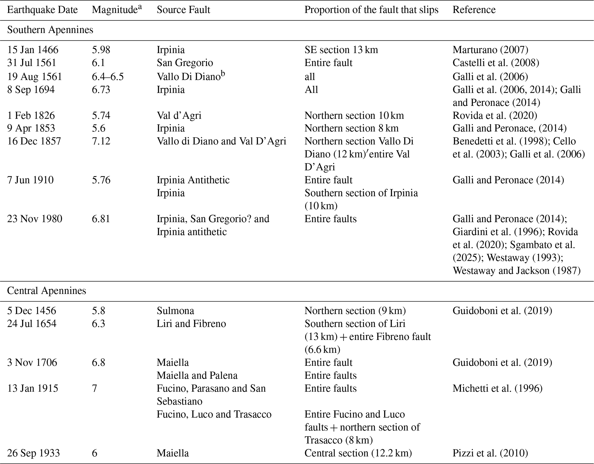
^a Magnitudes of seismic events in Central Apennines prior to 1979  A.D. are taken from the Catalogue di Forti Terremoti (Guidoboni et al., 2019) and are derived from the macroseismic shaking records (Gasperini and Ferrari, 2000) and as such are described as equivalent magnitudes (Me, based on Mildon, 2017). For more recent earthquakes in the Central Apennines post 1979 A.D. the magnitudes described are from seismological sources. ^b The name NW segment of Vallo di Diano often differs in the literature, being also known as Auletta fault or Caggiano fault (Bello et al., 2022; Galli et al., 2006)

Table B2 Paleoearthquakes and historical events in modelled faults of the Southern and Central Apennines.

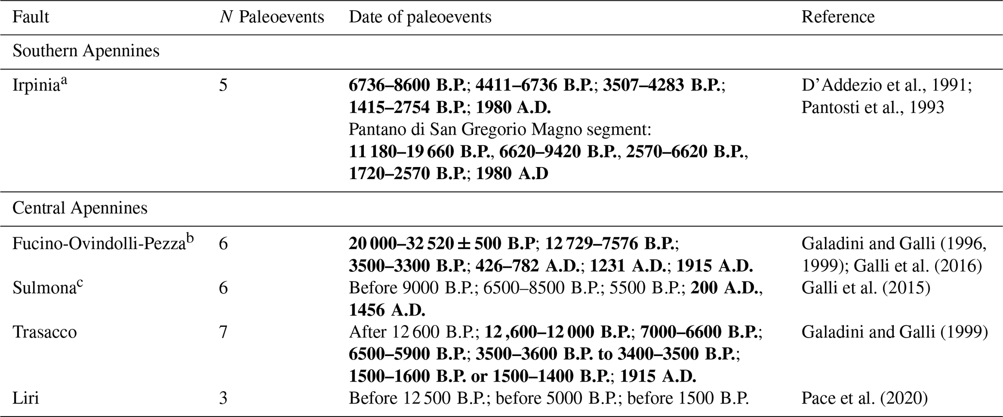
The nomenclature of some of the faults adopted by Faure Walker et al. (2021) and Sgambato et al. (2020b) and in this study differs from that of the paleoseismic data: ^a part of the Monte Marzano fault system by Galli (2020); ^b part of this fault is the San Benedetto dei Marsi–Gioia dei Marsi segment in the Fucino fault system in Galadini and Galli (1999); ^c also known as Monte Morrone fault by Galli et al. (2015). Paleoevents in bold are events with defined aged brackets used for the calculations of mean and standard deviation of recurrence times in the Discussion section.

Table B3 Comparison between recurrence times (mean and standard deviation in years) derived from historical and paleoseismological data (Tr_paleo) and modelled seismic events (Tr_model). Only paleoseismic events with well-defined age brackets were included in the calculation (see Table B2). Tr_paleo = recurrence times based on historical and paleoseismological data from the past 20 kyr. Scaled Tr_model = recurrence times from modeled seismic events adjusted by the correction factor.

Appendix C: SEAS simulations of Southern Apennines with nominal sip rate

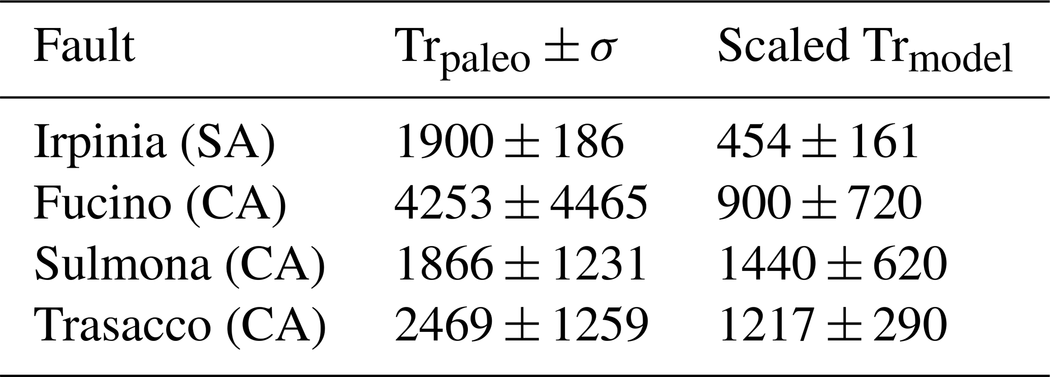
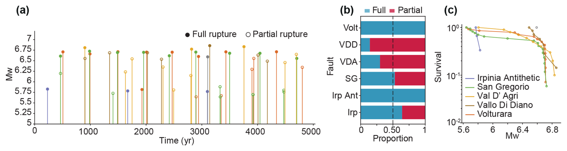
Figure C1 Synthetic catalog for a simulation of the Southern Apennines with nominal values of prescribed long-term slip rate. (a) Time distribution of simulated full- and partial-rupture events with stems and markers color-coded by fault (b). (b, e) proportion of full and partial ruptures per fault. (c) Magnitude-frequency distributions of seismic events shown as survival function (number of events with a M_w larger than a given value normalized by total number of events) for each fault. Color legend for each fault is shown in panels (c).

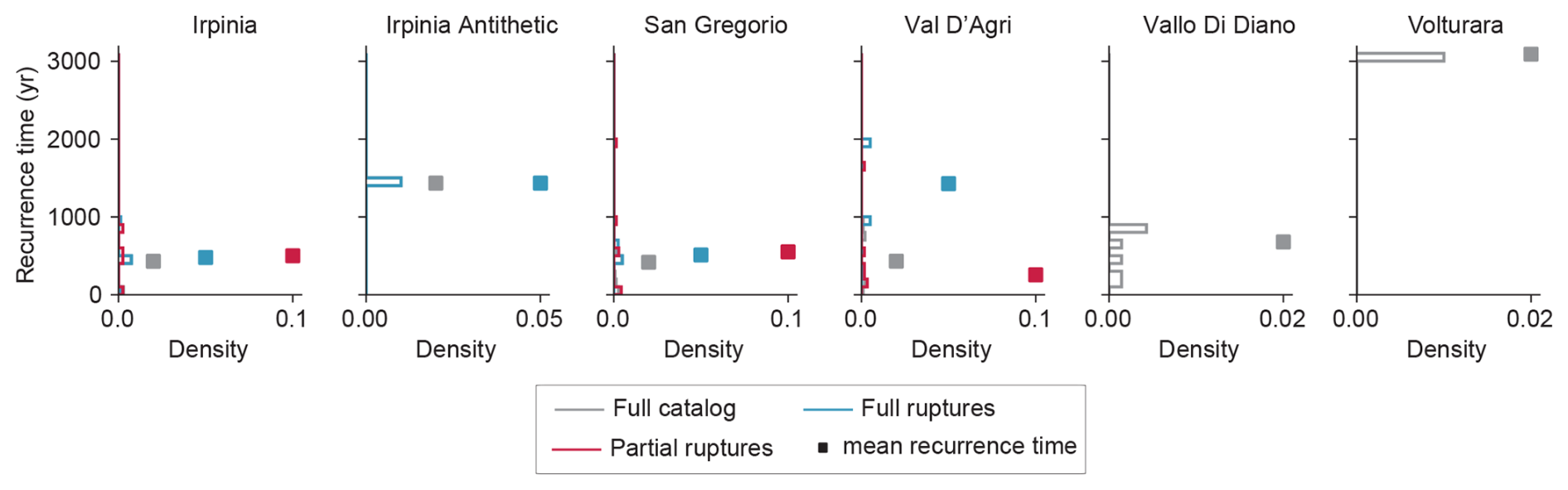
Figure C2 Variation of recurrence time of individual faults (step density histogram and mean recurrence time) and of the entire fault system for seismic events considering the full catalog, full-rupture and partial-rupture events of the fault networks for a simulation of the Southern Apennines with nominal values of prescribed long-term slip rate.

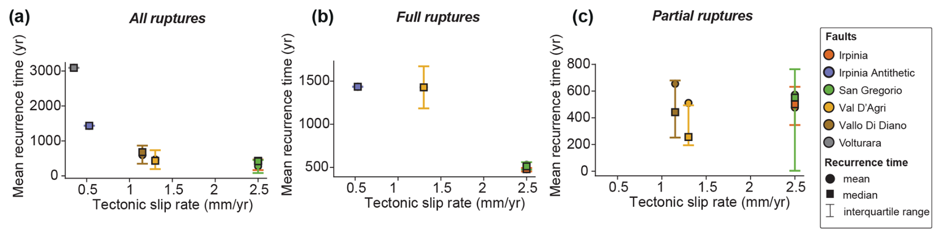
Figure C3 Mean, median and interquartile range of recurrence time of seismic events vs. (scaled) long-term tectonic slip rate of individual faults for a simulation of the Southern Apennines with nominal values of prescribed long-term slip rate.

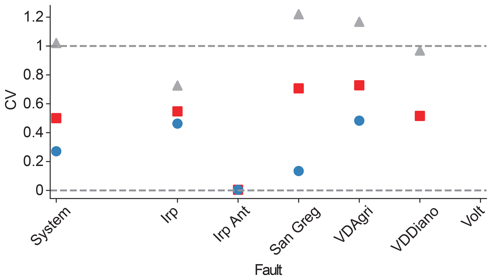
Figure C4 Coefficient of variation of recurrence times CV_Tr of seismic events (all events, only full ruptures and only partial ruptures) for individual faults and entire fault system for a simulation of the Southern Apennines with nominal values of prescribed long-term slip rate.

Appendix D: Determination of separation between faults

To determine the separation between two faults at depths of 0, 7.5 and 15 km we followed the following steps. First, for all fault traces, we created bounding transects normal to the fault tips (Fig. D1a). Second, for each fault pair, we drew a polygon bounded by two of the transects (one for each fault) and the fault traces (Fig. D1b). Third, we created sample lines (separation lines) equally spaced by 100 m parallel to the transects (Fig. D1c). Lines that did not intersect the fault traces or the transects were removed. Fourth, we clipped the sample lines to the polygon area (Fig. D1d and e). Finally, for each set of overlap and separation lines, we computed the average length (preferred value) and standard deviation. The workflow was carried out with QGIS (QGIS Development Team, 2009).

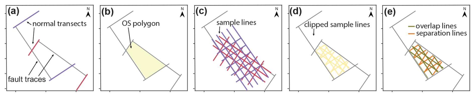
Figure D1 Illustrative workflow used to determine the separation between two fault traces at a given depth.

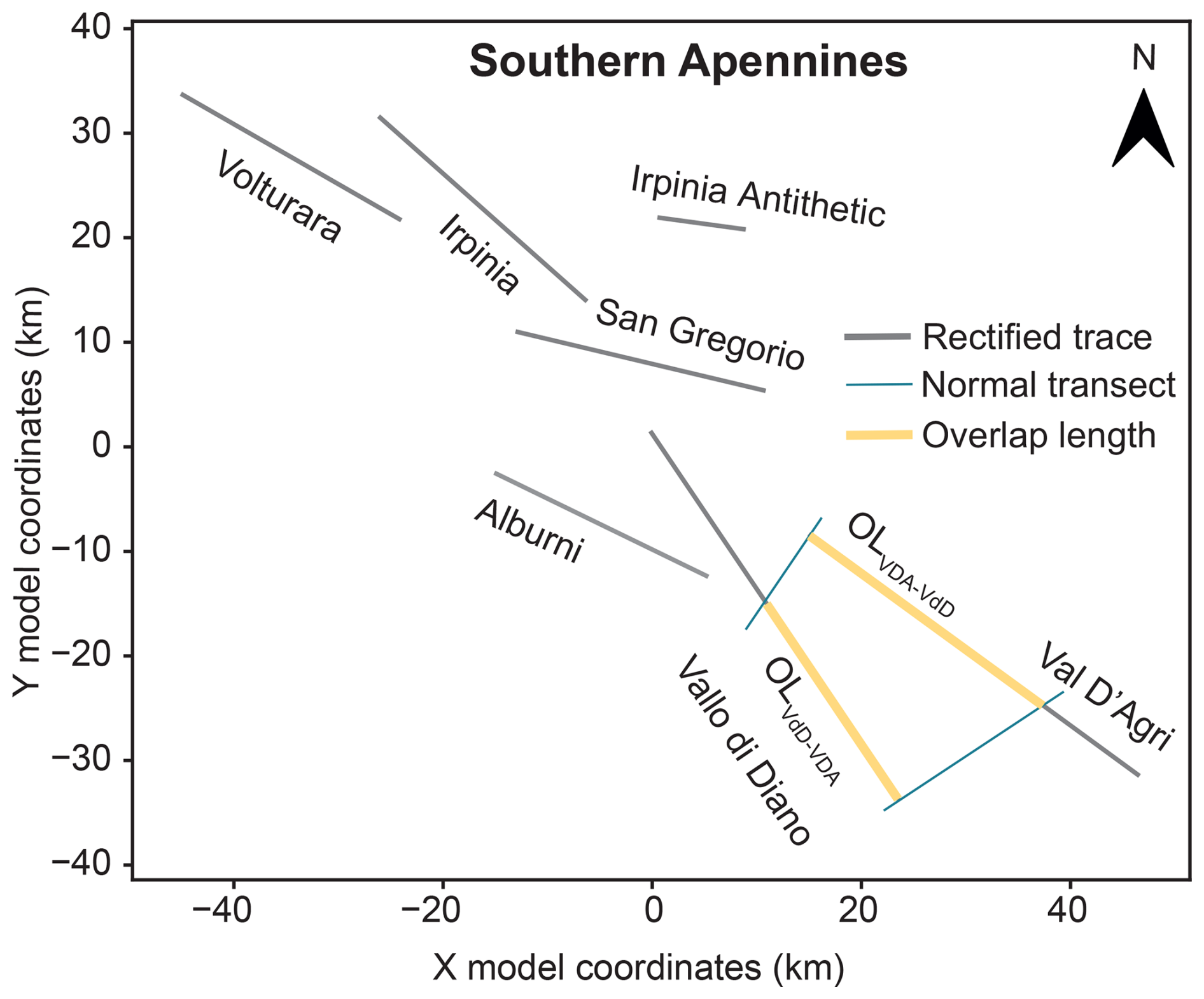
Figure D2 Determination of overlap length between two faults (in this example, Vallo Di Diano and Val D'Agri fault in the Southern Apennines) used for Figs. 7, E3 and E4. To determine the overlap length between two given faults (fault 1 and 2), we measure the distance along the strike of fault 1 between the normal transect to one of the tips of fault 1 to the normal transect of to one of the tips of fault 2.

Appendix E: Coseismic coulomb stress transfer

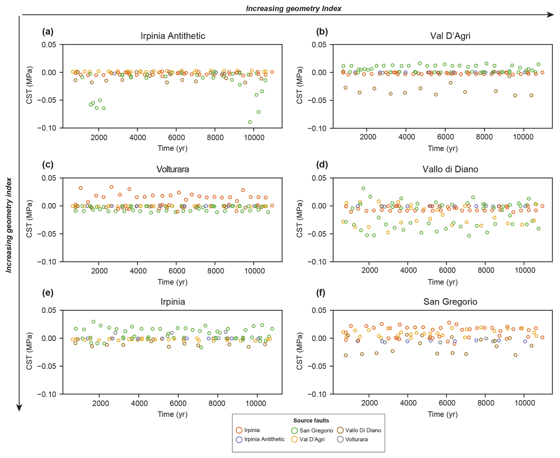
Figure E1 Time series with coseismic Coulomb stress transfer (CST) averaged across the fault surface induced by nearby faults in the Southern Apennines.

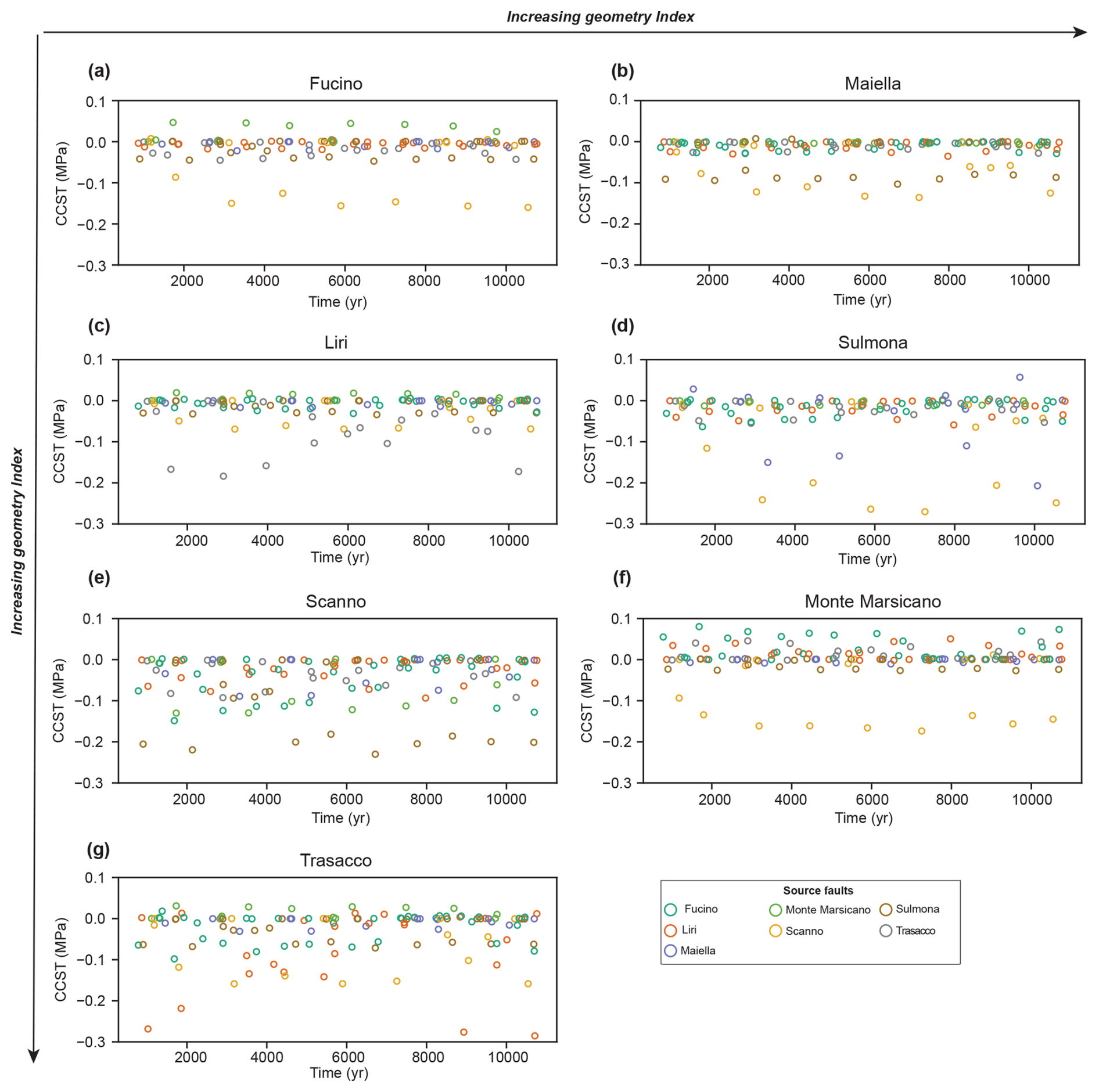
Figure E2 Time series with coseismic stress transfer averaged across the fault surface induced by nearby faults in the Central Apennines.

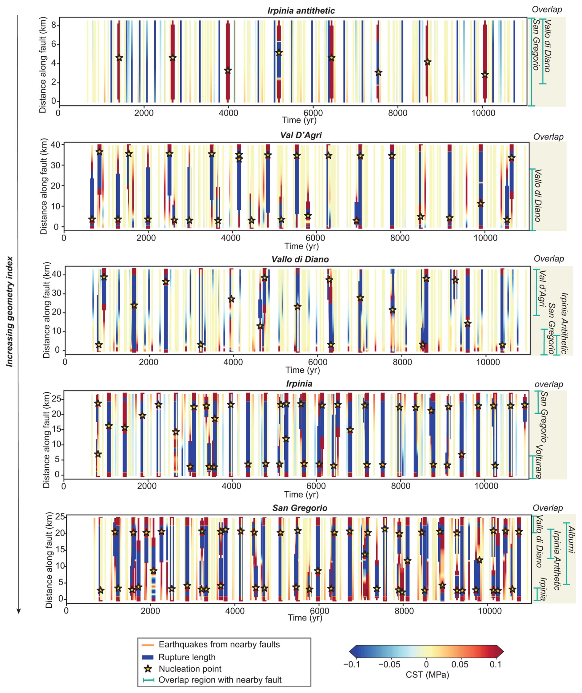
Figure E3 Coseismic stress transfer (CST) in the Irpinia Antithetic, Val D'Agri, Vallo di Diano, Irpinia and San Gregorio faults in the southern Apennines. For the figure explanation, see caption of Fig. 8 in the main text.

Figure E4 Coseismic stress transfer (CST) in the Maiella, Liri, Sumona, Scanno, Monte Marsicano and Trasacco faults in the Central Apennines. For the figure explanation, see caption of Fig. 8 in the main text.

Appendix F: Across-interaction index

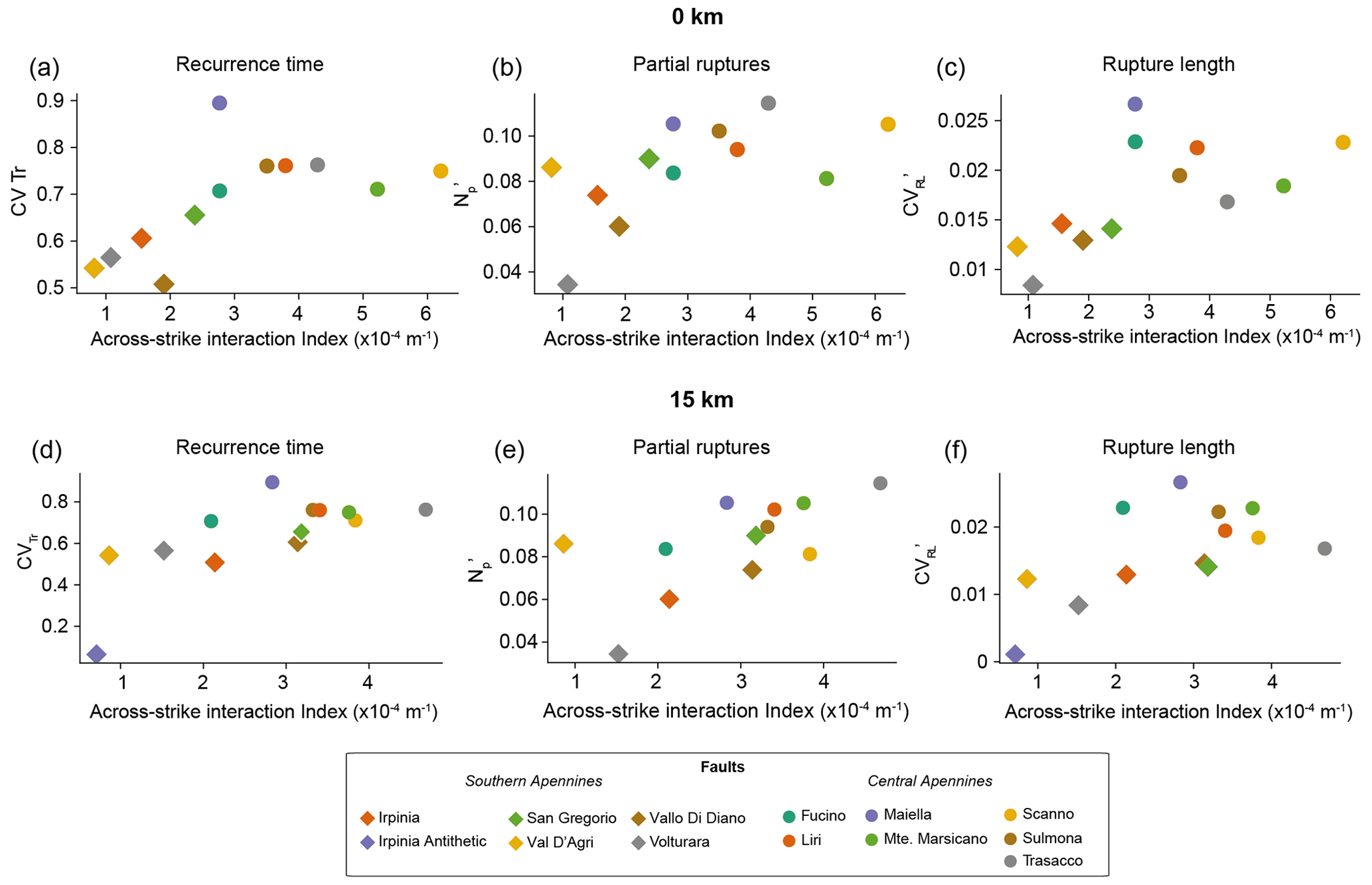
Figure F1 Relationships between fault network geometry, described by the across-strike interaction index (AI), and (a, b) coefficient of variation of recurrence times (CV_Tr), (b, c) number of partial ruptures ($N_{\mathrm{p}}^{\prime }$) and (d, e) coefficient of variation of rupture lengths (${\text{CV}}_{\text{rl}}^{\prime }$) for faults in the Southern and Central Apennines. AI index corresponds to a depth of (a, d, and e) 0 km and (b, d, and f) 15 km.

Table F1 Leave-one-out Spearman's correlation coefficients (mean, standard deviation, minimum, maximum) for relationship between across-strike interaction index (taken at 0, 7.5 and 15 km) and coefficient of variation of recurrence times (CV_Tr), number of partial ruptures ($N_{\mathrm{p}}^{\prime }$) and coefficient of variation of rupture lengths (${\text{CV}}_{\text{rl}}^{\prime }$) for faults in the Southern and Central Apennines.

Appendix G: Recurrence time and tectonic slip rate

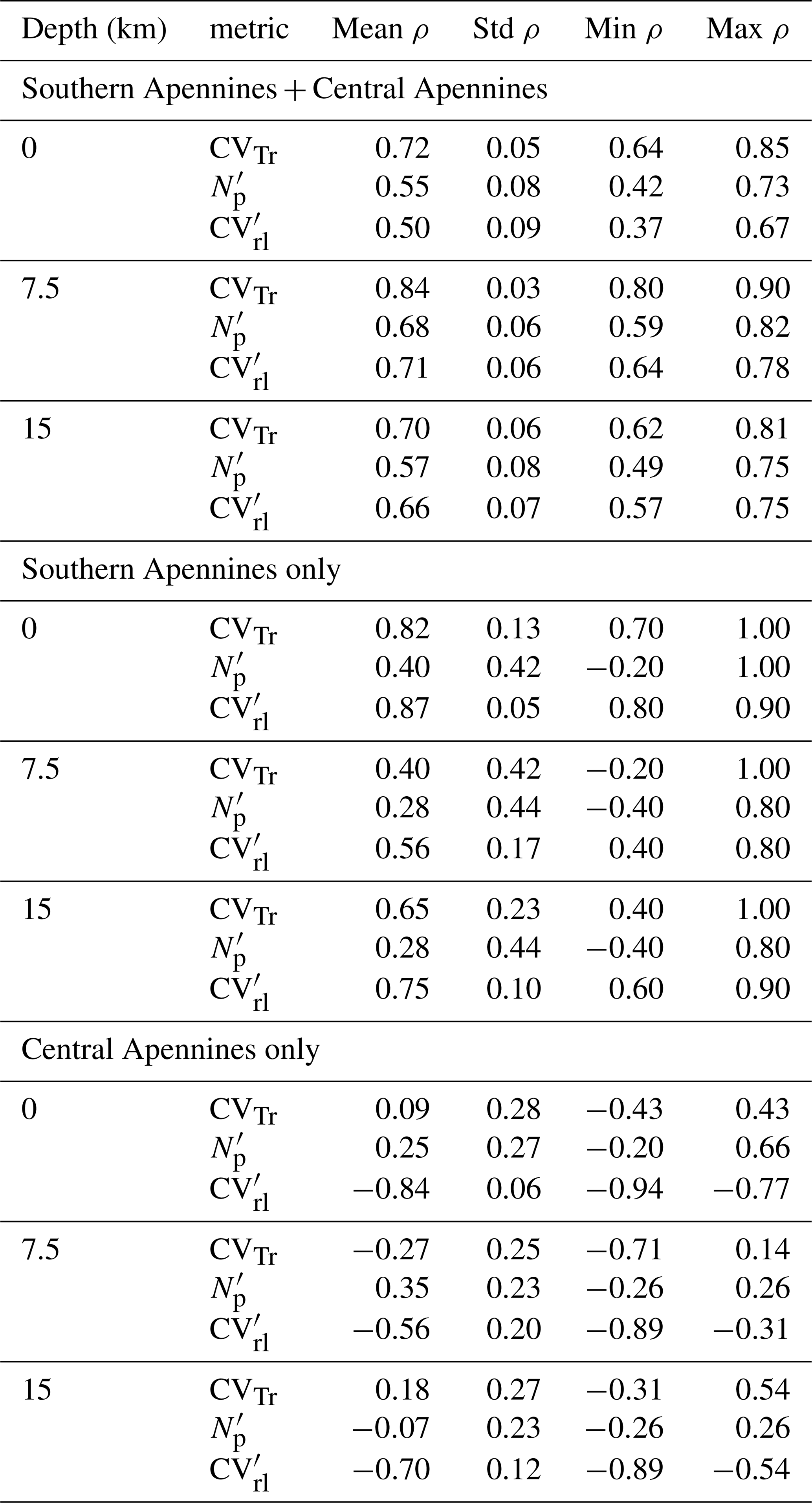
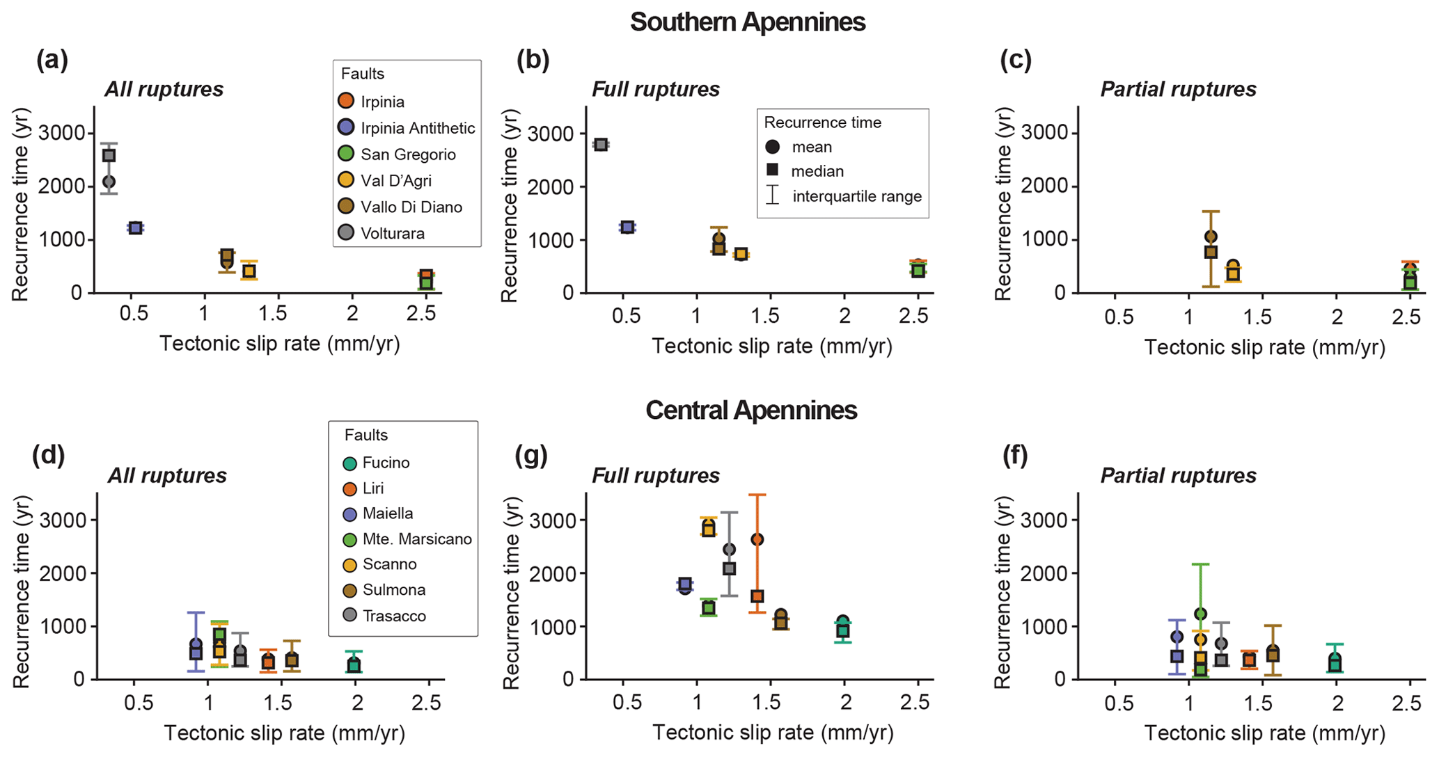
Figure G1 Mean, median and interquartile range of recurrence time of seismic events vs. long-term tectonic slip rate of individual faults for (a) Southern Apennines and (b) Central Apennines.

Appendix H: Calculation of magnitude-frequency distributions with the moment budget method

We estimate annual cumulative earthquake rates for individual faults and fault networks using the moment-budget (MB) and activity-rate (AR) tools implemented in the seismic-hazard code FiSH (Pace et al., 2016). This approach is based on the conservation of seismic moment over tectonic time scales, requiring information of the fault geometry and long-term slip-rate (Table 1). For each fault, the moment rate ${\dot{M}}_{\mathrm{0}}$ that must be released by earthquakes on the fault over time is calculated as:

$$\begin{array}{}\text{(H1)}& {\dot{M}}_{\mathrm{0}}=GA\dot{D}\end{array}$$

Where G is the shear modulus, A is the fault area derived from its geometry and $\dot{D}$ is the long-term slip rate. Earthquake magnitudes M_w are related to the seismic moment M₀ through the standard relationship of Hanks and Kanamori (1979):

$$\begin{array}{}\text{(H2)}& {\text{log}}_{\mathrm{10}}\left(M_{\mathrm{0}}\right)=\mathrm{1.5}{M}_{\mathrm{w}}+\mathrm{9.1}\end{array}$$

We used the truncated Gutenberg Richter formulation, where the incremental magnitude frequency distribution is defined as:

$$\begin{array}{}\text{(H3)}& v\left(M\right)=C{\mathrm{10}}^{-b(M-M_{min})},M_{min}\le M\le M_{max}\end{array}$$

Where b is the b-value (b=1), M_min the minimum magnitude ($M_{min}=\mathrm{5.5}$) and M_max the fault-specific maximum magnitude inferred from geometry. The constant C is determined by enforcing the moment conservation, such as the integral of the seismic moment released by the distribution is equal to the long-term moment rate:

$$\begin{array}{}\text{(H4)}& {\int }_{M_{min}}^{M_{max}}{M}_{\mathrm{0}}\left(M\right)v\left(M\right)\mathrm{d}M={\dot{M}}_{\mathrm{0}}\end{array}$$

From the incremental rates, we calculate the annual cumulative exceedance rate for each fault defined as the expected annual number of events with magnitude equal or greater than m:

$$\begin{array}{}\text{(H5)}& \mathit{\lambda }(M\ge m)={\int }_m^{M_{max}}v\left(M\right)\mathrm{d}M\end{array}$$

To obtain the exceedance rates per fault network, we summed the cumulative rates assuming independent Poissonian sources. Further details on this approach are provided in (Pace et al., 2016)