Deciphering the crustal structure of the Lerma Valley (NW Argentina): a multi-method seismic investigation

We investigated the crustal structure beneath the Lerma Valley in northwestern Argentina using data from a local seismic network deployed between 2017 and 2018. This geologically complex transition zone between the Eastern Cordillera and the Santa Bárbara system is characterized by moderate to high seismicity, yet remains largely understudied despite its strategic location within the Andean orogen. Its passive orogenic setting and evidence of inherited structures make it a natural laboratory for exploring intraplate deformation and foreland basin evolution. We combined local and teleseismic receiver functions with ambient noise tomography (ANT), jointly inverting Rayleigh wave phase velocities to obtain 1D shear-wave velocity profiles. The results reveal a stratified crust with four main discontinuities at $\sim \mathrm{53}-\mathrm{43}$, 35–30, 10–8, and 1.5–1.2 km, corresponding to the Moho, mid- and lower-crustal boundaries, and the sedimentary basin base. A southward-dipping Moho is evident from CCP migration and T-component phase shifts. Velocity profiles also show a north–south contrast: lower velocities (1–2.5 km s⁻¹) in the south indicate thicker, less consolidated sediments, while the north exhibits more competent crust (up to 3.5 km s⁻¹). The final model comprises five layers, including three sedimentary and two crystalline crustal units. We also introduced a layer-dependent κ correction, revealing a trend from 1.65 at the Moho to 2 in the upper layers. These results provide new geophysical constraints on the crustal architecture and tectonic evolution of this underexplored Andean region.

1 Introduction

The Lerma Valley, located in Northwestern Argentina, represents a geologically complex transition zone between the Eastern Cordillera and the Santa Bárbara system (Fig. 1a). Characterized by moderate to high and diffuse seismicity (INPRES, 2024) in comparison to its surrounding orogenic belts, this region exhibits unique tectonic features that remain largely understudied. Despite its strategic location within the Andean orogen, due to its mining and agronomic activities, and also being a densely populated province capital, no detailed geophysical or seismological investigations have been carried out in the valley, leaving significant gaps in our understanding of crustal deformation processes in this area (Jordan et al., 1983; Allmendinger et al., 1997). The basins current structural configuration suggests a passive orogenic regime, where deformation is not strongly controlled by active tectonics but rather by inherited structures and long-term crustal reorganization (Ramos, 2008). This makes it a natural laboratory for investigating the dynamics of passive orogen and the foreland evolution in continental interiors.

Geological evidence indicates that the Lerma Valley has undergone a complex tectonic history marked by Paleozoic basement uplift, Cenozoic basin development, and Quaternary fault reactivation (Mon and Salfity, 1995; Kley and Monaldi, 2002). These features offer a valuable opportunity to analyze the interplay between ancient tectonic inheritance and ongoing stress fields. The lack of systematic geophysical data, including seismic imaging, ambient noise tomography, and receiver-function analysis, underline the need for comprehensive studies aimed at understanding both its current rheologic and geodynamic behavior and its relationship with broader Andean processes. The integration of multidisciplinary geophysical approaches in the Lerma Valley holds the potential to shade some light on the mechanisms of intraplate deformation and the evolution of passive orogens–topics that remain poorly constrained at a global scale (Pérez et al., 2016; Tassara et al., 2018).

In this context, improving our knowledge of the crustal structure of the Lerma Valley in northwestern Argentina has important implications for the understanding of the Andean crustal characteristics, ongoing orogenesis, and isostatic processes. Moreover, the Lerma Valley and adjacent areas in the Santa Bárbara System has a very active seismogenic history with several destructive events with M_w>5. Recent events include the M_w 6.1 2010 Salta earthquake and the 1930 La Poma event (INPRES, 2024). In the Santa Bárbara System, historic 1692 Nuestra Señora de Talavera de Esteco (INPRES, 2024), the 1825 Anta (INPRES, 2024; Ortiz et al., 2022), and the M_w 5.8 2015 el Galpón earthquakes testify to the present-day seismotectonic activity that reflects the stress transfer from the active continental margin to the orogenic hinterland. The destruction related to the 2015 El Galpón earthquake and the damage-buildings suffered by the 2010 Salta earthquake are testimony of potential high-acceleration zones in this region. Recent studies conducted in the vicinity of the Salta city (in the center of Lerma valley) have revealed the presence of unconsolidated sediments within the first 25 m below the surface (Orosco, 2007; Orosco and Orosco, 2010). It has been demonstrated (Elías et al., 2022) that these sediments are susceptible to water saturation after heavy rainfalls during the austral monsoon season; these unconsolidated deposits have important implications for site effects and amplification phenomena.

The main tectonic structures of this area remain poorly constrained at depth, and they are very complex due to the existence of Cretaceous extensional faults that have been subjected to contractional inversion during Cenozoic Andean mountain building. A detailed characterization of the basin sediments is of paramount importance for further seismological and geotechnical applications and mitigation efforts. In addition, the deeper crustal structures are poorly known. For example, the boundaries for the upper, middle and lower crust were only studied for the northern and southern limit of the studied region. The thickness of the crustal units was first established by Cahill et al. (1992) in a study of the seismicity of the Zapla ranges in the province of Jujuy, which provided a depth of 42 km for the Moho. Thirty years later, Zeckra (2020) presented a model for the crust that placed the Moho at 46 km to the southeast of our study region. However, deriving detailed velocity models was not the aim of neither of these previous studies, as the models were derived from inversions of the travel times of seismic phases of local crustal earthquakes for better location.

The limitations of traditional seismic methods based on active seismic sources include their limited spatial coverage and the associated implementation costs. In contrast, ambient noise tomography (ANT) uses records of the seismic ambient noise wavefield at different locations to passively probe subsurface structures. By cross-correlating such records between two seismic stations, it is possible to extract coherent signals that are, under certain assumptions, proportional to the Green's function between the pair of stations, in addition it is worth to mention that unlike active seismic sources, the ANT are diffuse spatially and temporally (Wapenaar, 2004; Stehly et al., 2006; Bensen et al., 2007). As complementary information to that provided by the ANT (Green's functions and wave velocities), receiver functions (RF) contain information related to the seismic discontinuities in the subsurface, which can in turn be used in the inversion of velocity models based on the dispersion curves calculated for the surface wave part of empirical Green's functions (Julia et al., 2000).

The goal of this study was to develop a detailed velocity model that includes the lower, middle, and upper crust. This model was constrained by receiver function results and phase velocity dispersion curves (obtained from ANT); when jointly inverted these provide a local S-wave velocity model that accounts for the discontinuities at different scales. These discontinuities where then be compared to those proposed by previous studies for the uppermost units of the upper crust.

2 Geological setting

The studied area encompasses the Lerma Valley, an approximately 150-kilometer-long, north–south-oriented intermontane basin in the Eastern Cordillera of Argentina. The basin is flanked by basement-cored ranges (Pascha and Lesser ranges in the west, and Mojotoro-Castillejo-El Cebilar ranges in the east) delimited by reverse faults with both east and west vergence. These main structures correspond to inverted Cretaceous normal faults and Paleozoic faults which were reactivated during the Andean orogen (Grier et al., 1991; Mon and Hongn, 1991; Mon and Salfity, 1995). One of the most important structures in the area is the regional Calama-Olacapato-Toro (COT) lineament (1). This NW–SE trending structure crosses the Lerma Valley and could have exerted a tectonic control over the Paleozoic depostis and the Salta Group rift sequences to the north and south, respectively (Moya, 1988; Marquillas et al., 2005). Marrett and Strecker (2000) and Hongn and Seggiaro (2001) postulated a main transcurrent sinistral movement for this segment of the lineament, which could reflect the differential blocks movements both towards the north and the south.

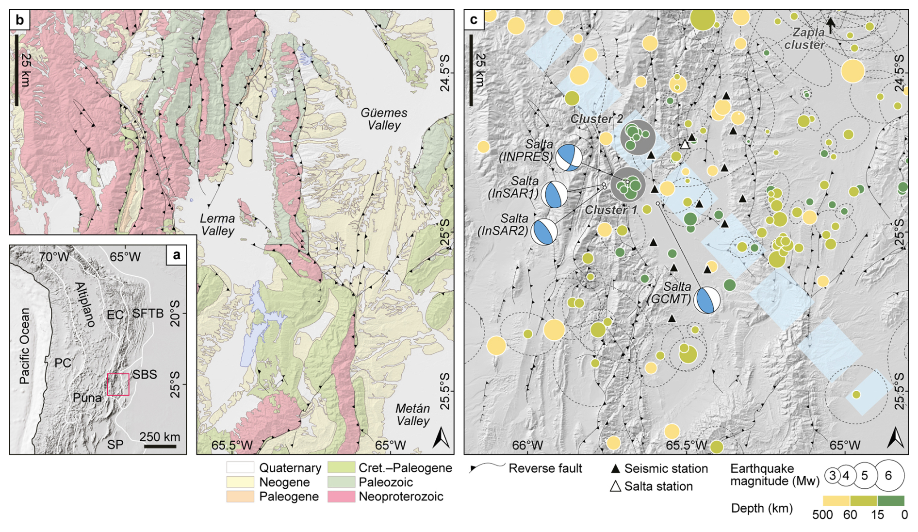
Figure 1 (a) Location map in context of the geological provinces: SFTB: sub-Andean fold-and-trust belt, AP: Altiplano-Puna, EC: Eastern Cordillera, SBS: Santa Bárbara System and SP: Sierras Pampeanas (modified after Jordan et al., 1983) (b) Lerma Valley, and surrounding valleys with lithologies and reverse faults Seggiaro et al. (2019). (c) LeVaRIS catalog (Criado-Sutti et al., 2017) discriminated by depth (in color) and magnitude (area), with focal mechanisms solutions provided by Scott et al. (2014). The light blue stripped line marks the COT (Calama-Olacapato-Toro) lineament (Salfity, 1985).

The stratigraphic succession that crops out along the valley and into the bounding ranges is composed of:

1. Neoproterozoic-Lower Cambrian metasediments of Puncosviscana Formation (Turner and Mon, 1979)

2. Cambro-Ordovician quartzites, marine shales and sandstones from the Mesón and Santa Victoria Groups (Turner, 1960)

3. Cretaceous-Paleogene rift deposits of Salta Group mainly composed of mudstones, sandstones and carbonates (Moreno, 1970)

4. Miocene-Pleistocene continental sequences from Orán Group that includes conglomerates and sandstones (Russo, 1972)

5. Quaternary fill of the valley was separated into three main units, the Calvimonte, Tajamar and La Viña Formations (Gallardo et al., 1996) formed by fluvial-alluvial and lacustrine deposits.

A comprehensive review of the stratigraphy of the Lerma Valley can be found in García et al. (2013).

3 Data and Methods

3.1 Deployment of the seismic network

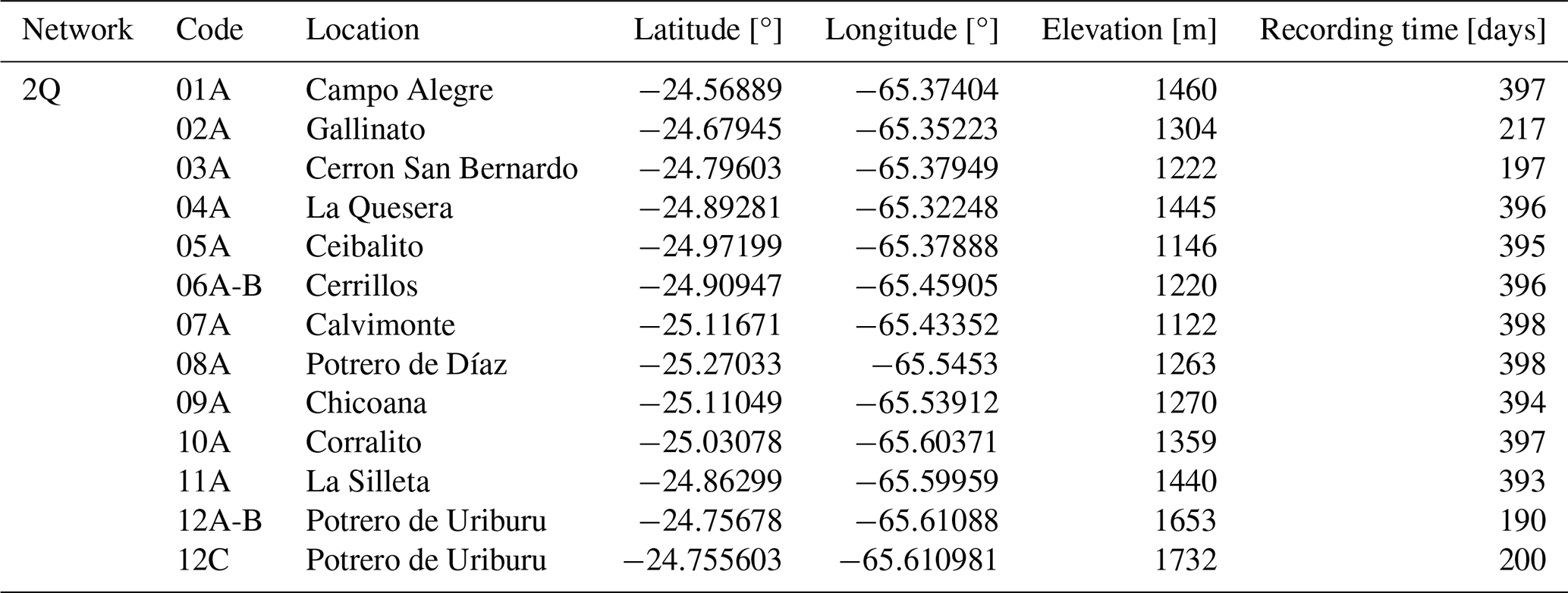
In August 2017, a temporary seismic network, composed of thirteen seismic stations, the Lerma Valley Ring Installation of Seismometers (LEVARIS, Criado-Sutti et al., 2017) was installed in the studied area. The network spanned the central and northern regions of the valley ($-\mathrm{24.558},-\mathrm{25.272};-\mathrm{65.623},-\mathrm{65.318}$) and operated for a total of thirteen months. Prior to this deployment, there was only one permanent short-period station within the valley, managed by Argentine agency INPRES (code SLA, INPRES, 2024).The dimensions of our temporary network spanned approximately 80 km in the north–south direction and 30 km in the east–west direction, with seismic stations strategically located to ensure safety, accessibility, and minimal interference from anthropogenic noise sources. The seismic stations were equipped with a DATA-Cube3 type digitizer paired with a Lennartz 3D/5s sensor. One of the installations (2Q.09A in Fig. 1) used a Mark L-4C-3D short-term seismic sensor. In all cases, instruments were buried at an approximate depth of 60 cm. The Data-Cube3 digitizers were set to a sampling rate of 100 Hz, and the seismic stations were powered by batteries connected to solar panels.

Table 1 Location of the seismic stations of the LEVARIS temporary network, with their approximate recording time in days.

3.2 Methods

In order to study the various discontinuities of the crust below the grater Lerma Valley and to derive local velocity models, we employed three methods: receiver functions analysis (teleseismic and local), ambient noise cross-correlation tomography, and joint inversions (forward modeling). The first two methods involved processing the raw data from the LEVARIS network (see Sect. 3.1, Criado-Sutti et al., 2017) to produce receiver functions and dispersion curves. Then latter results were combined to be inverted using forward modeling and fitting the data to the S-wave velocity model, thus obtaining a representative crustal model. In the following sections we present and briefly describe each method and also provide a complete description of the parameters used in the data processing.

3.2.1 Teleseismic Receiver Functions (RFs)

As seismic waves from distant earthquakes (teleseisms, from 30–90° distance) travel through the Earth's interior, they can undergo reflections and P-to-S conversions at interfaces, such as the crust-mantle boundary (the Moho). Receiver function (RF) analysis enables the detection of these converted phases, providing insights into the subsurface structure beneath the region covered by a seismic station.

The “RFs” method, originally developed for teleseismic analysis (Langston, 1977; Vinnik, 1977; Burdick and Langston, 1977), involves the deconvolution of the vertical component from the horizontal components of a rotated seismogram to isolate the Earth's impulse response (Ligorría and Ammon, 1999) beneath the seismic station. This procedure suppresses the effects of the source-time function and distant propagation path, highlighting converted arrivals such as the Ps phases. Arrival times of these converted phases can be associated with structural discontinuities, provided that a reference velocity model is available.

To improve spatial resolution and imaging of discontinuities such as the Moho, Common Conversion Point (CCP) stacking is employed. CCP stacking allows a pseudo-migration of RFs from the time domain to depth by tracing converted phases back into the Earth along theoretical ray paths using a local velocity model. This approach helps account for lateral heterogeneity and enhances structural imaging, particularly when focusing on strong, isolated phases like Ps, which are typically more prominent and interpretable than crustal multiples (Dueker and Sheehan, 1997; Audet, 2015).

3.2.2 Local Receiver Functions

Local deep earthquakes provide a complementary and, in several respects, more diagnostic source for receiver function (RF) analysis than teleseismic events. Their shorter source durations and enriched high-frequency content result in shorter dominant wavelengths, which enhance sensitivity not only to sharp velocity contrasts but also to strong impedance variations associated with highly fractured or damaged zones within rocks of otherwise similar bulk composition (Langston, 1979; Bostock, 1998; Rondenay, 2009). Such zones may produce coherent converted phases or scattered energy that are strongly attenuated or entirely smeared out in lower-frequency teleseismic RFs.

This sensitivity to fine-scale heterogeneity makes local RFs particularly effective for imaging tectonically damaged crust, shear zones, and transitional boundaries where fracturing and fluid content, rather than major lithological changes, dominate seismic contrasts (Hansen et al., 2013). In addition, the steep incidence angles of waves generated by deep local earthquakes reduce lateral averaging of converted phases, further improving the resolution of subhorizontal discontinuities such as the Moho and intracrustal interfaces.

In the study region, the application of local RFs is especially advantageous because deep seismicity is concentrated within the Jujuy cluster, with hypocentral depths of approximately 200 km (blue dots in Fig. 2) (Mulcahy et al., 2014; Valenzuela Malebran, 2022). This source geometry provides dense and narrowly focused sampling of the crust beneath the LEVARIS stations, despite the limited lateral extent of the earthquake cluster. As a result, local RFs offer high-resolution constraints on crustal thickness and internal structure, including the Moho, which lies at depths of 40–50 km in this region (Cahill et al., 1992; Zeckra, 2020), and supply an independent test of interpretations derived from teleseismic RFs.

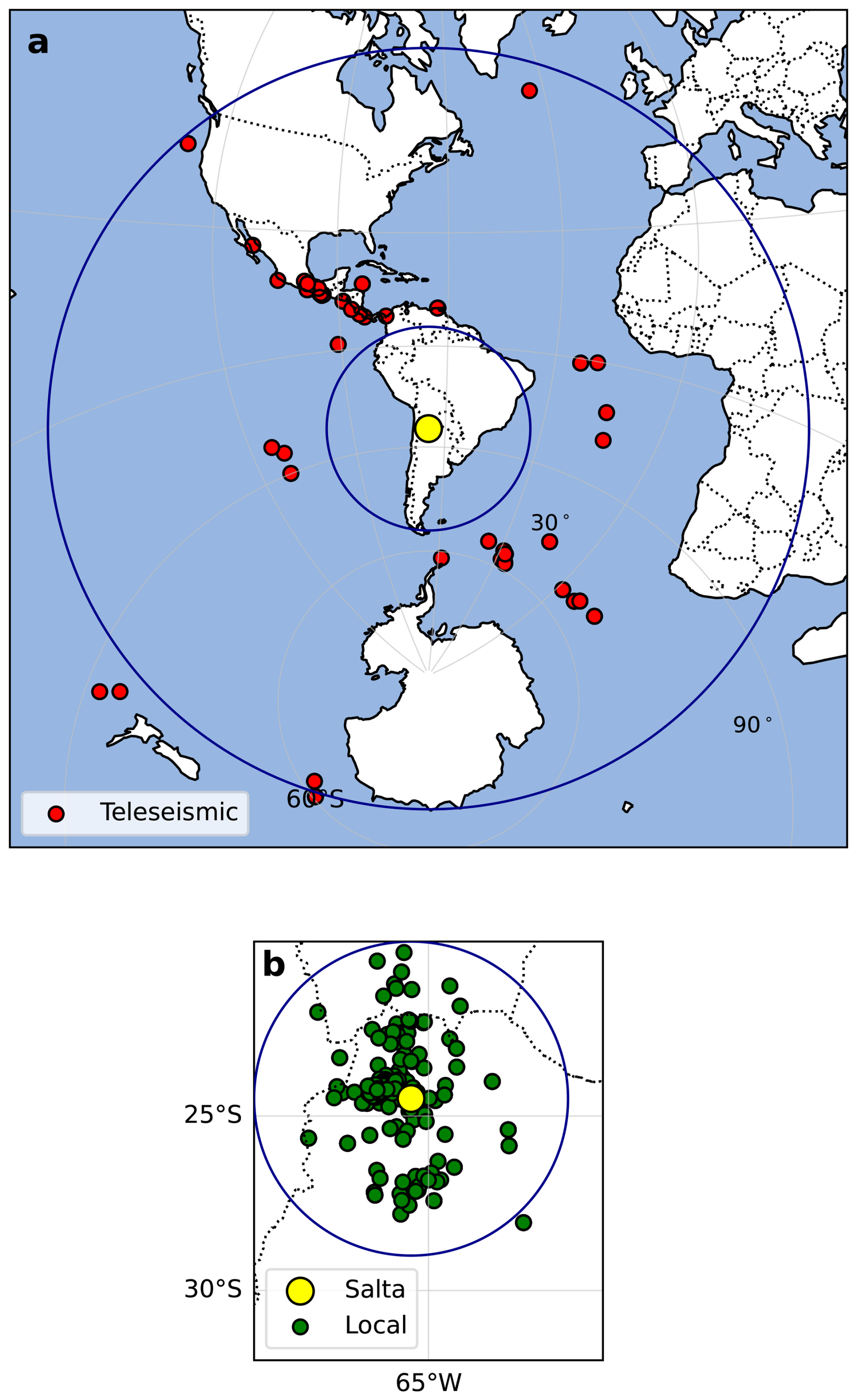
Figure 2 Events distributions for teleseismic (a, red) and local (b, green) events used for the receiver functions in an equidistant plot.

Local deep earthquakes ($M_{\mathrm{L}}\in [\mathrm{1.5},\mathrm{4}]$, depth ∼200 km) were analyzed using the same general workflow, with the main difference being the event catalog, which was constructed specifically for this study based on the LEVARIS network (Criado-Sutti et al., 2017).

3.2.3 Teleseismic and Local RF Parameters Setting

For both teleseismic and local events, we applied a bandpass filter from 0.01–2.0 Hz to isolate the relevant frequency band. To ensure data quality, we extracted 300 s noise windows ending 10 s prior to the P-wave arrival and computed the RMS of both noise and signal windows, discarding traces where the RMS ratio was below 1.5. Deconvolution was performed using the water-level method (e.g., Langston, 1977), with a Gaussian filter width of a=0.5 and a water-level parameter of c=0.1. A subsequent manual inspection step was used to remove traces with excessive noise or anomalous amplitudes. The resulting quality-controlled receiver functions were used to identify P-to-S converted phases and to estimate crustal properties, including Moho depth and $v_p/v_s$ ratio, via the H−k stacking technique (Zhu and Kanamori, 2000).

3.2.4 H−k Analysis

The H−k stacking method, introduced by Zhu and Kanamori (2000), is a widely used technique for estimating crustal thickness (H) and the $v_p/v_s$ ratio (k) by analyzing teleseismic receiver functions. The method relies on identifying the arrival times of converted and multiple seismic phases, such as Ps, PsPs, and PpSs. When appropriate values of H and k are found, the sum of the amplitudes of the receiver functions at the corresponding travel-times interfere constructively, allowing the determination of crustal discontinuities by locating maxima in the stacking function.

In our implementation, we assumed a fixed P-wave velocity of 6 km s⁻¹ (average of the crust). The analysis was performed on a grid with 2 km increments in depth (H) and 0.05 increments in the $v_p/v_s$ ratio (k). The bounds of the grid search were set from 0–70 km for H and from 1.6–2.5 for k. These parameter ranges and step sizes were selected to ensure adequate resolution while maintaining computational efficiency. We estimated the uncertainties in the parameters H and k following the method of Eaton et al. (2006), who proposed defining a contour line at one standard error below the maximum stack amplitude. The standard error is given by $({\mathit{\sigma }}^{\mathrm{2}}/N{)}^{\mathrm{1}/\mathrm{2}}$, where σ² is the variance and N is the number of stacked receiver functions. This method implies that confidence in the estimated parameters increases with the number of receiver functions included in the stack.

3.2.5 Estimation and Adjustment of Effective k Values

The H−k technique yields only an average $v_p/v_s$ ratio (k) above a given discontinuity. To capture its depth dependence, we compute an effective k_eff(H) using a 1D velocity model with depth-varying v_p and v_s, defined as the ratio of their travel-time integrals down to depth H:

$$\begin{array}{}\text{(1)}& k_{\text{eff}}\left(H\right)={\displaystyle \frac{{\int }_{\mathrm{0}}^H\frac{\mathrm{1}}{v_s\left(z\right)}\mathrm{d}z}{{\int }_{\mathrm{0}}^H\frac{\mathrm{1}}{v_p\left(z\right)}\mathrm{d}z}}.\end{array}$$

Uncertainties are estimated by propagating bounds on H:

$$\begin{array}{}\text{(2)}& {\mathit{\sigma }}_k={\displaystyle \frac{\mathrm{1}}{\mathrm{2}}}\left|k_{\text{eff}}\right(H_{\text{max}})-k_{\text{eff}}(H_{\text{min}}\left)\right|.\end{array}$$

This formulation provides a physically consistent comparison with measured k, which assumes constant velocities. The measured k can be interpreted as a velocity–thickness weighted average of individual layer contributions. For a stack of n layers with thickness H_i, P-wave velocity v_p,i, and ratio k_i, the effective value is

$$\begin{array}{}\text{(3)}& k_{\text{meas}}^{\left(n\right)}={\displaystyle \frac{{\sum }_{i=\mathrm{1}}^n{k}_i\cdot v_{p,i}\cdot H_i}{{\sum }_{i=\mathrm{1}}^n{v}_{p,i}\cdot H_i}}.\end{array}$$

This relation allows reconstruction of depth-dependent k_i values through a bottom-up recursive scheme using known v_p,i, an assumed average 〈k〉 at the Moho, and layer thicknesses. However, the method assumes vertical incidence of seismic waves; deviations (e.g., ∼15°) introduce systematic bias due to longer ray paths. For typical crustal velocities, this may lead to an overestimation of k of about 5 %, highlighting the need to account for incidence angle effects when interpreting results.

3.2.6 Ambient Noise Tomography (ANT)

To estimate empirical Green's functions between receiver pairs within the LEVARIS network, we applied ambient noise cross-correlation techniques to continuous seismic data (Table 1). The available recordings were segmented into two-hour windows, detrended, cosine-tapered (5 %), and corrected for instrument response. Cross-correlations were then computed by spectral multiplication in the frequency domain, following the method of (Ekström, 2014):

$$\begin{array}{}\text{(4)}& {\mathit{\rho }}_{ijk}={\displaystyle \frac{u_{ik}\left(\mathit{\omega }\right)u^{jk}\left(\mathit{\omega }\right)}{\sqrt{u_{ik}\left(\mathit{\omega }\right)u^{ik}\left(\mathit{\omega }\right)}\sqrt{u^{jk}\left(\mathit{\omega }\right)u_{jk}^{*}\left(\mathit{\omega }\right)}}},\end{array}$$

where ρ_ijk is the cross-correlation for stations i and j in time window k, u represents the Fourier-transformed time series, and ^* denotes complex conjugation. The resulting cross-correlograms were stacked across the entire deployment period, and a time-scale phase-weighting scheme (Ventosa et al., 2017) was applied to enhance signal-to-noise ratios prior to further analysis.

The ambient noise dataset from the LEVARIS network was organized using the Pyrocko-based “jackseis” tool (Heimann et al., 2019), with daily MiniSEED files sorted by component and stored in annual station-specific folders using Julian day naming conventions. Cross-correlations were computed as described above for all possible vertical-component station pairs using 1 h windows with 50 % overlap, and were then stacked over the entire deployment period to improve coherence. Dispersion measurements were obtained using time-frequency analysis to pick group velocities, following the method of Bensen et al. (2007), and phase velocities were estimated by numerical integration. To address the 2πN ambiguity in phase velocity curves, we selected the curve that remained closest to the corresponding group velocity without being slower, as recommended by Bensen et al. (2007).

Subsequently, the derived dispersion curves were used to produce surface wave tomographic maps based on the method of Barmin et al. (2001), which assumes surface waves propagate along great-circle paths between stations. The tomographic inversion was conducted in two stages. In the first inversion, strong regularization parameters were applied (α=1000, β=50, and σ=400 km) to generate oversmoothed velocity maps for quality control, following procedures outlined in Barmin et al. (2001). Measurements that deviated by more than two standard deviations from the mean phase or group velocity were flagged and removed. A second inversion was then performed using the same regularization parameters to produce the final phase velocity maps. The regularization involved a balance between smoothing and fidelity to the data, and parameter values were chosen through trial-and-error (Barmin et al., 2001), with visual inspections confirming that small perturbations in the chosen parameters did not significantly affect the resulting maps.

3.2.7 Joint Inversion of RFs and Phase Velocity Dispersion Curves using Hamiltonian Monte Carlo (JIHMC)

The Hamiltonian Monte Carlo (HMC) inversion method (Betancourt and Girolami, 2015; Betancourt, 2018) provides a robust framework for exploring complex posterior distributions by leveraging an energy-based sampling approach that minimizes the misfit between observed and synthetic data. This technique is particularly well-suited for seismic inversion problems due to its ability to efficiently explore high-dimensional parameter spaces with strong correlations.

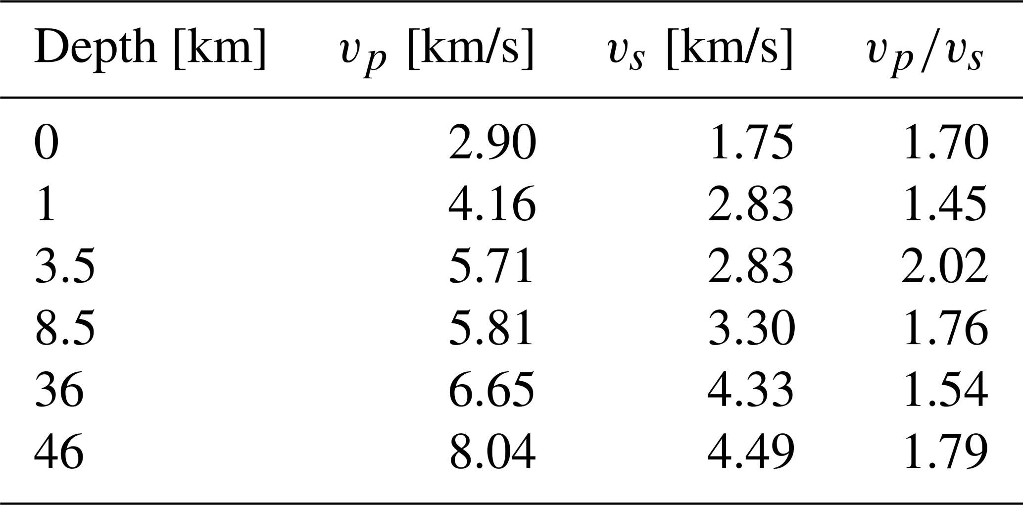
For our local model inversion, we adopted a modified version of the velocity structure proposed by Zeckra (2020) as a baseline (Table 2). Although alternative velocity models were considered, including a preliminary 1D velocity model derived from a VELEST inversion of local events, these alternatives proved unstable and were ultimately not used.

Table 2 Modified velocity model derived from Zeckra (2020), with the second layer subdivided into two layers of 1 and 3.5 km thickness, showing depth, P- and S-velocities, and $v_p/v_s$ ratios.

The joint inversion was carried out using the RfSurfHmc software package (Quang-Duc, 2021), a Python-based framework with C-based computational kernels that implements the HMC approach developed by Betancourt and Girolami (2015) and Betancourt and Girolami (2015)) and later integrated with the EvodCinv platform (Luu, 2018). The RfSurfHmc (Quang-Duc, 2021) tool enabled the simultaneous inversion of teleseismic receiver functions and phase velocity dispersion curves to construct station-specific shear wave velocity profiles.

The input data included stacked receiver functions in the time range from 0–10 s and surface wave dispersion curves from 1.7–10 s. Inversions were performed using data from all LEVARIS seismic stations (see Fig. 1) to resolve broader basin-scale features. The inversion was run for 200 iterations, with misfit weighting parameters set to ${\mathit{\sigma }}_{\text{rf}}=\mathrm{1}\times {\mathrm{10}}^{-\mathrm{3}}$ for receiver functions and ${\mathit{\sigma }}_{\text{swd}}=\mathrm{0.7}\times {\mathrm{10}}^{-\mathrm{2}}$ for surface wave dispersion curves.

The forward modeling step used a Gaussian filter with parameters a=1.5 and c=0.001, and a time step of dt=0.1 s. We used a ray parameter of $\mathrm{0.045}\mathrm{s}/\mathrm{°}$ and explored the depth range from 0–50 km ($L=\mathrm{0}-\mathrm{50}\mathrm{km}$). These parameter values were selected after a series of empirical tests in which each parameter was varied by approximately ±10 % around the reference configuration. For each tested setup, synthetic receiver functions were computed and compared with the observations. The final parameter set was retained because it consistently led to a better fit to the observed receiver functions than the alternative configurations tested (see Appendix).

3.2.8 Inversion of Surface Wave Phase Velocity Dispersion Curves with Evolutionary Algorithm (IEA)

Evolutionary algorithms (EAs) are optimization techniques inspired by the principles of natural selection and genetics. These methods are particularly well suited for exploring large, complex solution spaces where conventional optimization strategies may struggle due to non-linearity, high dimensionality, or multimodal objective functions (Mitchell, 1998; Deb, 2001). EAs have seen widespread application in various fields such as machine learning, computational biology, and geophysical inversion (Sambridge and Drijkoningen, 1992), offering a flexible and robust approach to finding globally optimal solutions (Mitchell, 1998; Deb, 2001).

In this study, we employed an evolutionary algorithm to invert surface wave phase velocity dispersion curves, following the approach described by Luu (2018). This method was particularly effective in enhancing resolution in the upper five kilometers of the crust, where conventional methods often lack sensitivity.

The inversion was carried out on phase velocity dispersion curves measured over periods ranging from 1.7–9.9 s. The evolutionary algorithm was initialized with a population size of 20 and a random seed set to zero to ensure reproducibility. The optimization process was iterated for a total of 200 generations. These settings were chosen based on prior benchmarking (Luu, 2018) to ensure a balance between computational efficiency and solution robustness.

4 Results

In this section and the sections that follow, we present the results of our multi-methodic analysis of the Lerma Valley. In order to provide further support for these features, we have included a supplementary material that accounts for RFs, H−k analysis, ANT (path maps), and joint inversion.

4.1 H−k Analysis

The solution obtained from the H−k analysis showed to be stable and constrained in depth for both teleseismic and local receiver functions station stacks, which resulted in good results, for the deepest discontinuities at $\sim \mathrm{53}-\mathrm{43}$ and $\sim \mathrm{36}-\mathrm{30}\mathrm{km}$. However, the k values fluctuated considerably for the local receiver functions for the layers above the shallower $\sim \mathrm{10}-\mathrm{8}$ and $\sim \mathrm{1.5}-\mathrm{1.2}\mathrm{km}$ discontinuities. In Fig. 3 we present the results for the Moho defined from the teleseismic receiver functions for stations 01A and 05A. These two stations were selected because they show representative results, however the results for the other seismic stations are available in pickle format.

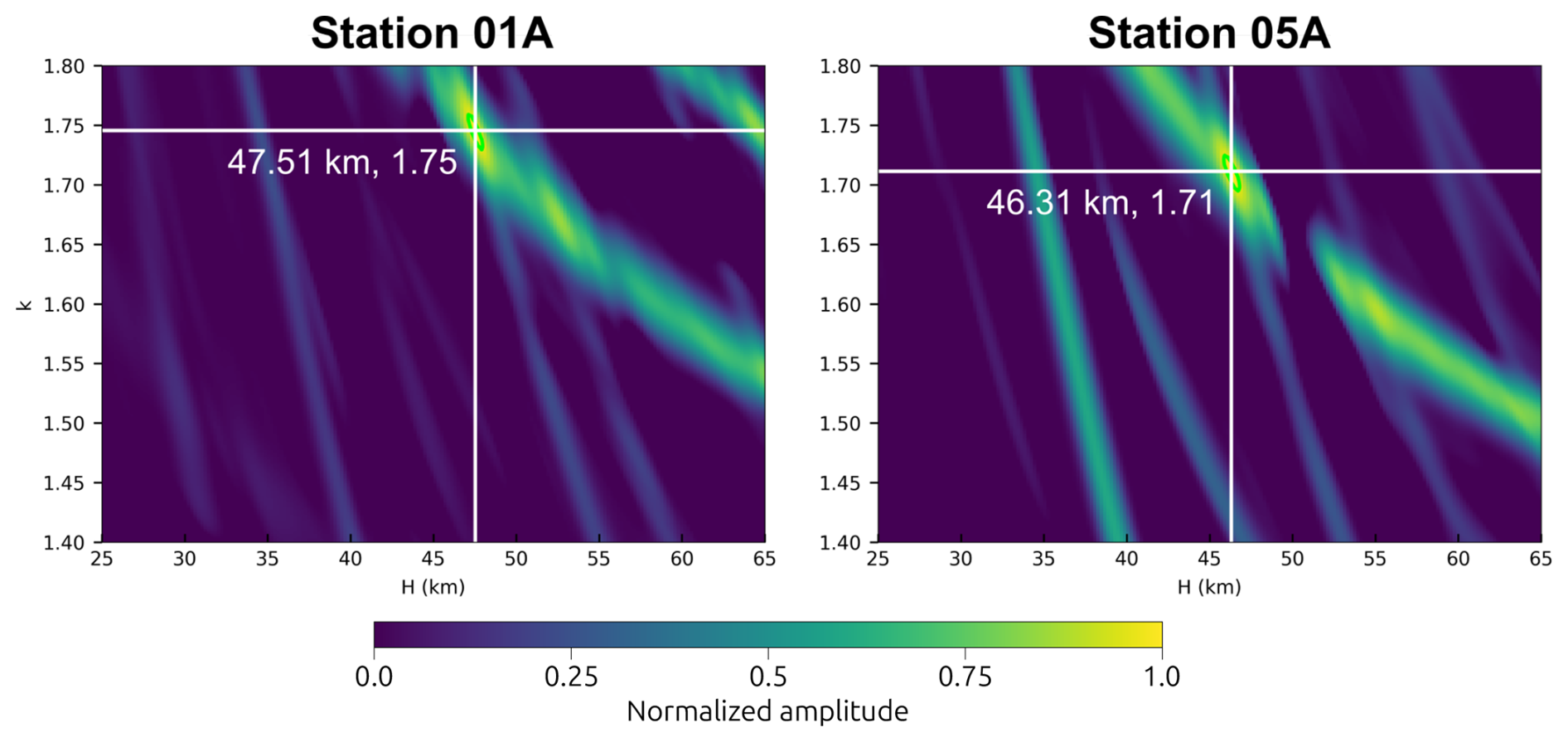
Figure 3 Sample H−k stacking results for stations 01A and 05A. The white lines indicate the position of the maximum value.

We see in Fig. 3 that the depth of the Moho discontinuity and the k parameters are well constrained. The $v_p/v_s$ ratio is the one expected for the Moho's region, being ∼1.75. For receiver functions calculated from local events the estimated Moho depths for the seismic stations shown in Fig. 3 are similar but the average $v_p/v_s$ ratios are slightly lower (see Table 3).

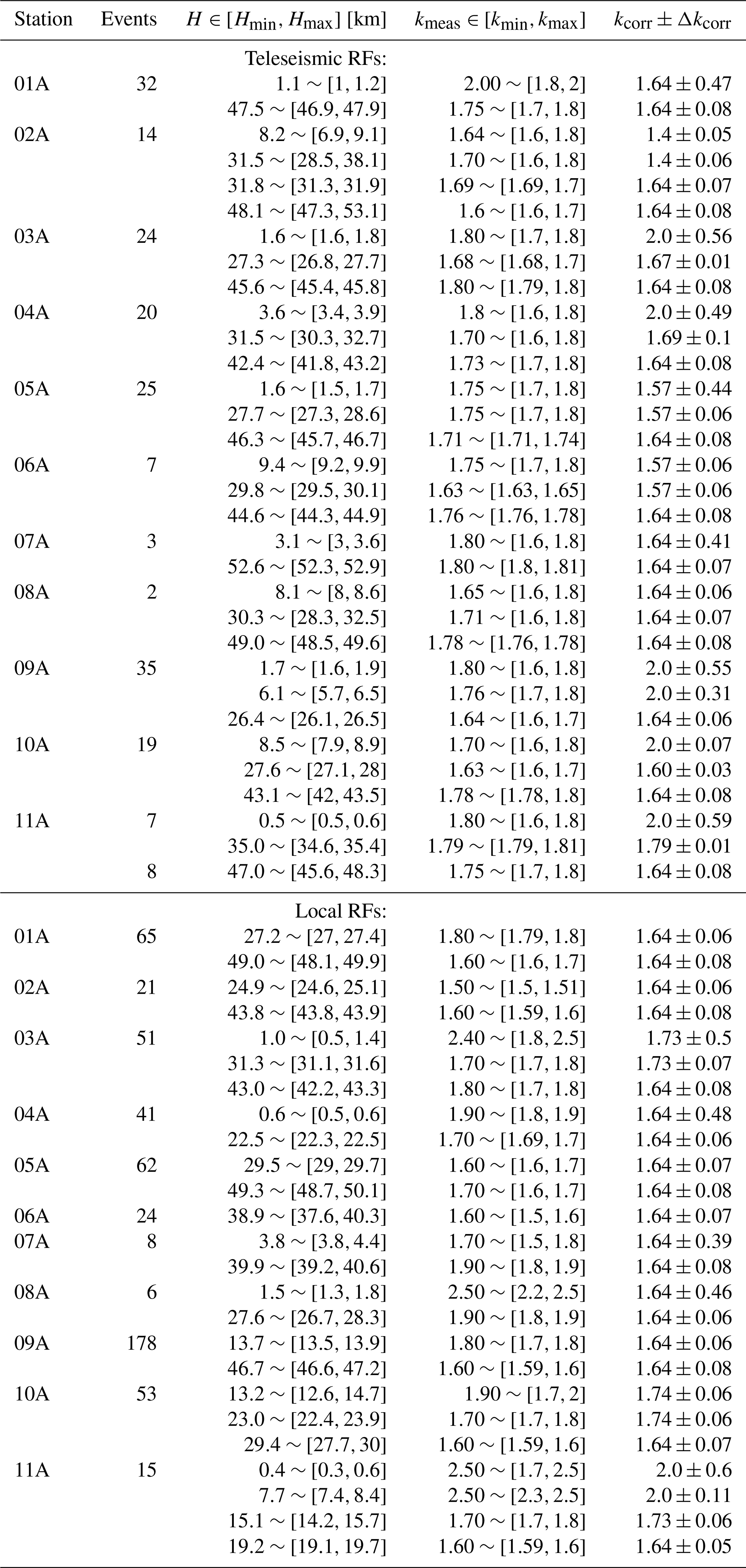
Table 3 Corrected $v_p/v_s$ ratios at each depth and station for teleseismic and local receiver functions, with depths H and measured k and their related error. $v_p/v_s$ ratio of 1.64±0.02 used at the Moho.

4.2 Receiver Functions

Figure 4 shows the receiver functions for station 01A for the radial Q and transversal T components, marking the Moho conversion times for Ps on the Q component at about 5 seconds. The traces were then stacked using a binning of 15° in backazimuth with an overlap of 5°. In the T components there is a clear azimuthal conversion near 200° at 2.5 s, evidently more present in the local RFs.

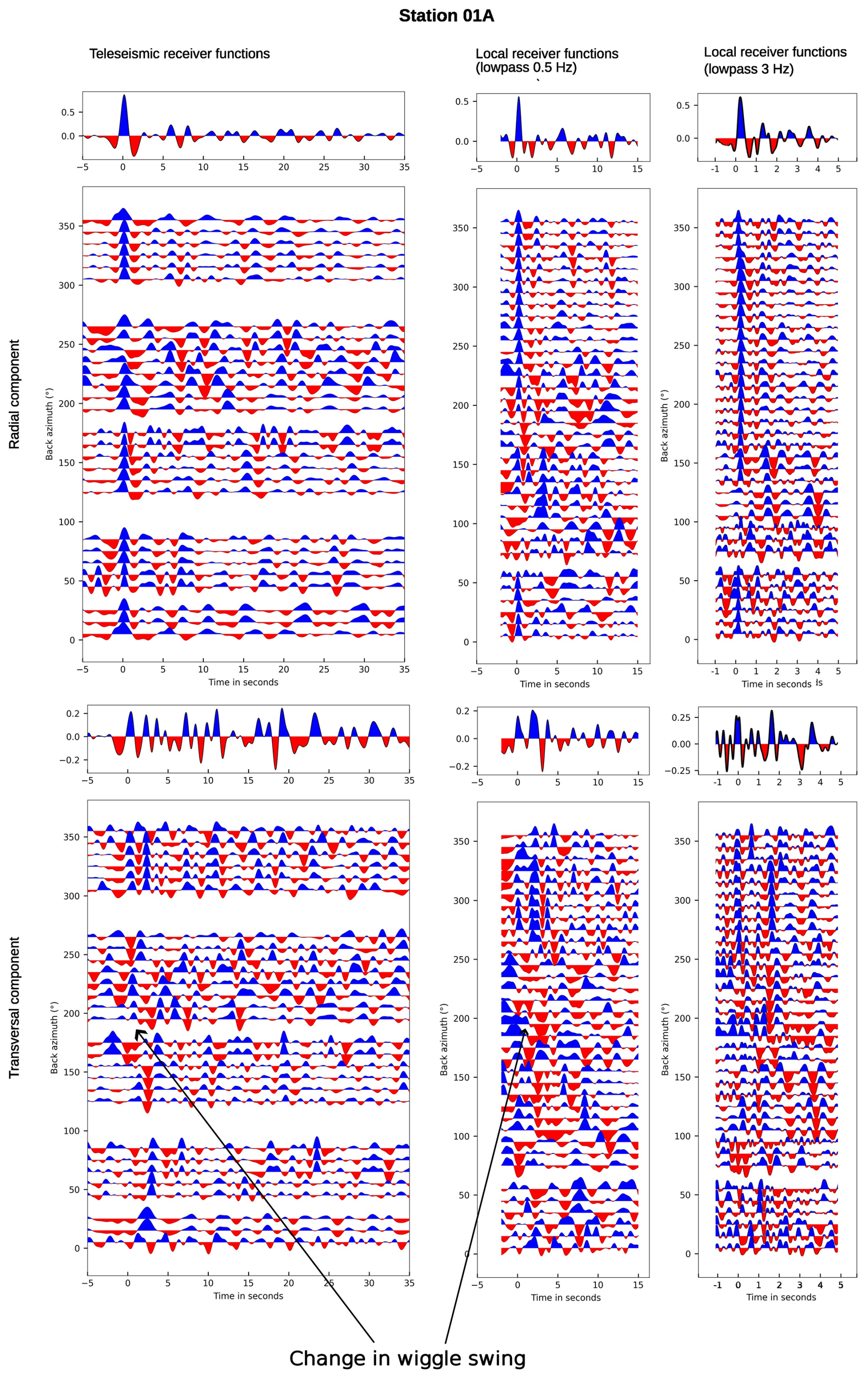
Figure 4 Teleseismic and local receiver functions computed for station 01A. The individual receiver functions are binned in 10° intervals, with an overlap of 5°. The linear stack is represented on top of each panel. The first row shows the radial component, while the bottom row shows the transverse component. The arrows mark a change in the wiggle swing at 200° approx.

4.2.1 Discontinuities

In Table 3 presents a comprehensive overview of all potential discontinuities for each station, spanning the shallow 1−2 km depth range up to the deeper 43−53 km region of the Moho, extracted from the H−k analysis of the stacked receiver functions. Specifically, four discontinuities were identified, from the lowest to the greatest depth: 43–53, 30–35, 8–10, and 1.2−1.5 km. The k values were corrected using the velocity model by Zeckra (2020). It is crucial to acknowledge that the majority of these discontinuities are not identifiable simultaneously for all stations. This is only the the case for the Moho Ps conversion which is visible at all stations. The errors for the deeper discontinuities are better constrained than those for the shallower discontinuities, showing values of less than 5 % relative error for both parameters, H and k (see Fig. 5). For the upper discontinuities, within the shallower interval of 1.2−1.5 km, i.e. the upper most layer, the resulting k-values were significantly increased in relative error, representing from 50 %–70 % of the measurement.

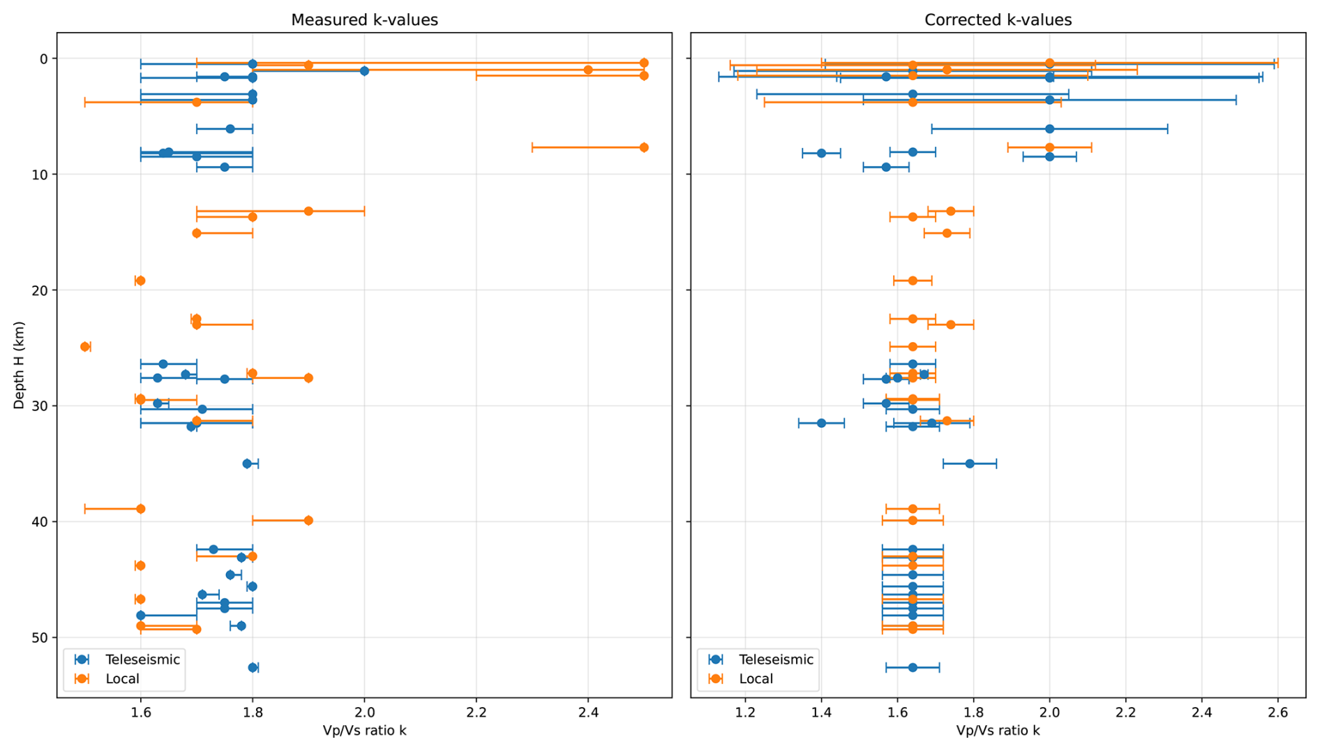
Figure 5 Measured and corrected k values as a function of depth for local and teleseismic events.

4.2.2 Corrected k-values

In Fig. 5, we present the results of our recursive correction method, where the vertical variation of the $v_p/v_s$ ratios can be observed. The corrected k values show less scatter than the apparent k values and both teleseismic and local event based receiver function sets agree now better. The k value is observed to slightly increase from 1.65 up to 2.0, from the Moho to the upper layers, although it is poorly constrained, particularly in the uppermost layer.

4.2.3 CCP results

Finally, Common Conversion Point (CCP Tessmer and Behle, 1988) results (see Fig. 6) clearly reveal four discontinuities, which are listed in Table 3, appearing as continuous zones. In the north–south profile $A-A^{\prime }$, three of these discontinuities – located at approximately 47, 30, and 10 km depth – are observed in both local and teleseismic RFs, with sharper resolution in the local RFs. Additionally, a discontinuity at around 15 km depth is identified exclusively in the local RFs. In both profiles, the Moho region thickens and dips southward, reaching depths exceeding 50 km.

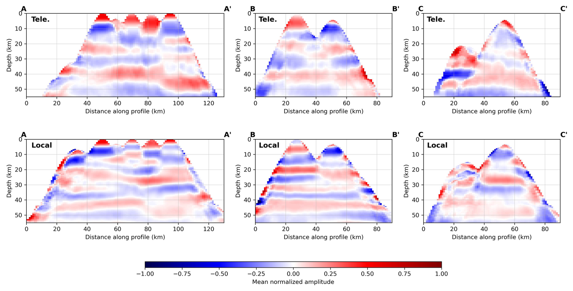
Figure 6 Pseudo-migrated sections of teleseismic (Tele.) and local (Local) receiver functions using the CCP stacking technique. The locations of the cross sections are shown in Fig. 9.

For the east–west directed profiles $B-B^{\prime }$ and $C-C^{\prime }$, situated in the south and north respectively (see profiles in Fig. 7), the same discontinuities are identified. However, in the northern profile, they appear more diffuse. Notably, the higher frequency content of the local RFs significantly enhances the clarity of structures in the east–west profiles.

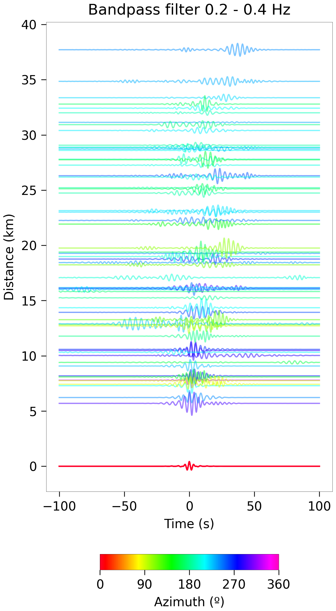
Figure 7 Acausal and causal parts of the cross-correlation for each station pair in terms of the inter-station distance band-passed with corner frequencies 0.2–0.4 Hz.

4.3 Ambient Noise Cross-correlation

Figure 7 shows the acausal and causal parts of the ambient noise cross-correlation traces in terms of the inter-station distance, where there is a clear one-sided tendency towards positive times. This, in principle will appear to be a contraposition to the homogeneity assumption of the ambient noise wavefield on which ANT is based. However, Pedersen and Krüger (2007) showed that even in this scenario of a dominant noise direction the cross-correlations are not significantly affected (less than 10 %). On the other hand, this also points to clear difference between the northern and southern sectors.

A combination of phase and group velocities of Rayleigh waves was obtained from the cross-correlations. The maps, computed for periods of 10 s, showed similar characteristics within the above time span (see Fig. 8). However, the quality of the phase velocities proved to be more consistent for shorter periods, particularly between 1.6 and 2.2 s. As a group, the velocities in all cases have an unstable (sharp oscillatory) behavior in the processed periods.

For the period of 2 s (see Fig. 8a and b), a weak zone of relatively slow velocities appears between the area enclosed by the stations 09A-07A-08A and 12A-06A-10A. This zone is only visible in the phase velocity maps. On the other hand, the group velocity shows a zone of relatively high velocity in the line formed by stations 12A-11A-10A and a zone of relatively low velocity in the area bounded by stations 06A-05A-07A-08A-09A. For the period of 3 s (see Fig. 8c and d), two distinct zones appear in both group and phase velocities: A zone of high relative velocity in the area bounded by stations 01A-02A-04A-05A-06A-03B, which will be called the northern sector, and a zone of relative low velocity between stations 11A-07A-08A-10A, which will be called the southern sector. The maps for the period of 4 s (see Fig. 8e and f), show for the high velocity zone an increase in contrast and extension in the group velocity map, and a decrease in extension and contrast of the low and high velocity zones in the phase velocity map. Finally, for the period of 5 s (see Fig. 8g and h), the two zones of high and low velocity, show a decrease in the velocity contrast.

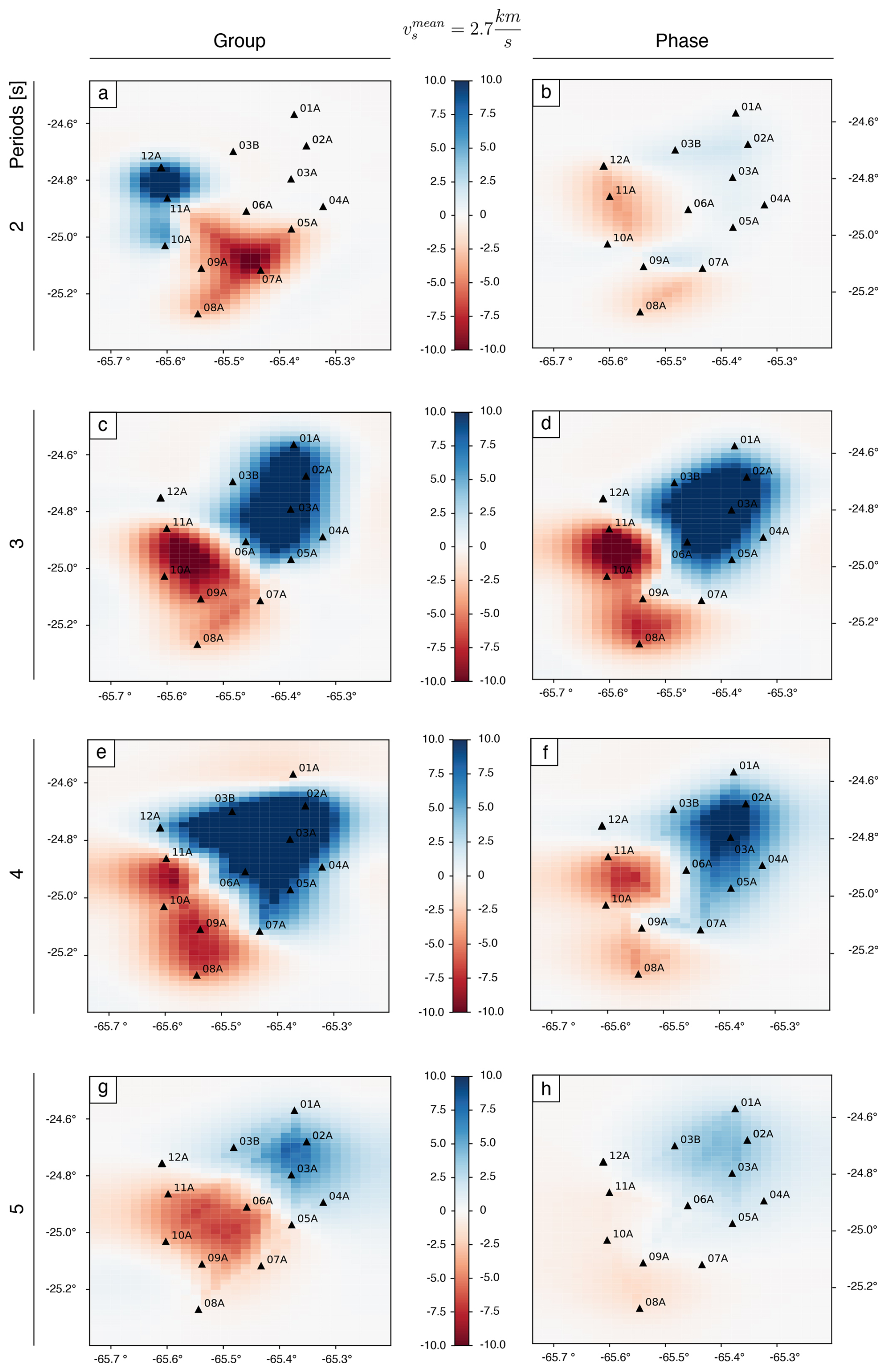
Figure 8 Group and phase velocity maps as function of period ranging from 2–5 s with station locations.

4.4 Joint Inversion

We observe that the best model derived from the joint inversion of RFs and dispersion curves reproduces the model proposed by Zeckra (2020) with the main difference that velocity of the shallowest layer are decreased to lower values and the discontinuities at 35 and 46 km change slightly to increased depths.

In Fig. 9, we present the inversion results for stations 01A, 05A, 07A and 10A. All four stations share similar depth and velocity characteristics, though subtle differences emerge. Notably, the upper layers in the northern region (station 01A) exhibit slightly higher S-wave velocities compared to those in the south, while the lower layers show consistently lower velocities compared to the reference model across all four stations without significant variation.

Figure 9 Base model (Zeckra, 2020, in red), VELEST model (in green) and best model inversion (in blue) for four representative stations; 01A, 05A, 07A and 10A namely.

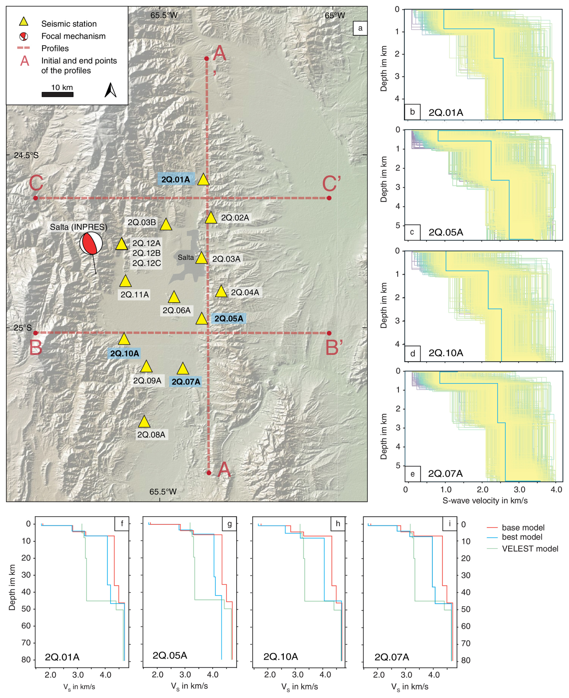
The receiver function fits are reliable for the selected stations, with station 05A displaying the best fit. At this station, the model closely follows the observed data, capturing not only the shape but also the amplitude of all maxima and minima.

Moreover, the results from the evolutionary algorithm inversion (see Fig. 9) align well with those from the joint inversion in the middle of the upper layers, between 3 and 5 km depth. A primary distinction is the presence of a low-velocity layer with shear wave velocities between 0.7 km s⁻¹ and 1 km s⁻¹, that varies in thickness, from 0.7–1 km, being thicker for station 10A (see Fig. 9).

The combined velocity model for all stations comprises five distinct layers: an upper sediment layer (0.8 km thick), below it a consolidated sediment layer (3.7 km thick), followed by a lower consolidated sediment layer (2 km thick), then an upper crustal layer (32 km thick), and finally a lower crustal layer (10 km thick). The Moho is located at a depth of 48–49 km.

5 Discussion

5.1 Moho Depth and Crustal Composition

The results presented in the previous section (see Sect. 4) highlight the complexity of the crustal structure in the Lerma Valley on multiple levels. In this trend, the discontinuities identified through the H−k analysis of the receiver functions (both teleseismic and local) align well with previously proposed regional crustal models, e.g. by Cahill et al. (1992). Specifically, regarding the depth of the Moho, all stations showed constrained and stable solutions at 48±5 km, a feature that aligns closely with the findings of Zeckra (2020), who positioned the Moho depth at 46 km in the Santa Bárbara system. Similarly, the corrected $v_p/v_s$ ratios remained in the range of 1.5–1.8, with a mean value of 1.65. This value also agrees with the results of Zeckra (2020), who attributed this ratio to a dry felsic composition in the lower crust. However, this low $v_p/v_s$ ratio is stable also for the upper discontinuities in the teleseismic receiver function results, as teleseismic signals, due to their long-period frequency, are less sensitive to minor changes in layer velocities. In contrast, local receiver functions reveal a gradual increase in the $v_p/v_s$ ratio from 1.64–2.0, spanning from the Moho upward. This behavior is also present in Zeckra (2020), where a $v_p/v_s$ ratio of about 2 is measured for the second layer.

5.2 Moho Geometry and Azimuthal Variations

In addition to the dry felsic layer identified above the Moho region, expressed by the low $v_p/v_s$ ratio of about 1.65, there is a shift in azimuth in the T components of the receiver functions indicates a dip along the north–south axis, centered around 200°. As shown in Fig. 2 for both local and teleseismic data, this feature suggests a gradual change in the Moho surface. Similar observations have been reported in New Zealand Savage (1998), where azimuthal analysis of receiver functions revealed Moho dips associated with variations in the geometry of the subducting plate.

5.3 Middle Crust Discontinuities

Moving to the middle crust discontinuities, the one at an average depth of 30 km appears well defined in teleseismic receiver functions but more dispersed in local receiver functions, likely represents the mid-lower crustal boundary. This finding is consistent with the velocity model of Zeckra (2020). Further, a discontinuity at 15 km depth, exclusive to local receiver functions, likely marks an upper detachment horizon with an extensive fracture network occupying the middle crust. Notably, similar features have been proposed on different scales by Grier et al. (1991), Kley and Monaldi (2002), and Pearson et al. (2013). This distinction by the local receiver functions is due to the high-frequency content in the spectra of Zapla cluster events (Mulcahy et al., 2014; Valenzuela Malebran, 2022).

5.4 Upper Crust Structure and Sedimentary Layers

Within the upper crust, a discontinuity at approximately 8 km depth is clearly imaged in the teleseismic receiver functions and at one station in the local dataset, whereas shallower interfaces between 5 and 1 km depth are consistently observed in both RF types. The deeper of these features likely reflects a first-order rheological contrast within the upper crust, which is preferentially resolved by long-period signals and may correspond to the transition from consolidated basement to overlying sedimentary sequences. Comparable depths for the sediment–basement transition (6–10 km) have been reported in seismic reflection and refraction studies across the Eastern Cordillera and adjacent foreland basins (Kley et al., 1996; Cristallini and Allmendinger, 2006).

In contrast, the shallower discontinuities are interpreted as marking the structural basement of the basin, represented by the Puncoviscana Formation (see Sect. 2), overlain by the Santa Victoria and Mesón Groups, the Salta Group, and younger Orán Group and Quaternary deposits. Stratigraphic and geophysical constraints indicate that the cumulative thickness of these sedimentary units commonly ranges between 3 and 7 km in the Lerma Valley and surrounding regions (Salfity, 1985; Hongn and Seggiaro, 2007).

5.5 Seismic Velocity Constraints and Basin Structure

Independent constraints from ambient-noise cross-correlation tomography reveal two seismic velocity domains in the uppermost crust, characterized by a low-velocity zone ($\sim \mathrm{1.75}\mathrm{km}{\mathrm{s}}^{-\mathrm{1}}$) and an underlying high-velocity zone ($\sim \mathrm{3.5}\mathrm{km}{\mathrm{s}}^{-\mathrm{1}}$). Similar velocity contrasts and thicknesses (1–4 km for low-velocity basin fill overlying higher-velocity sedimentary or metasedimentary units) have been documented in surface-wave and refraction studies in the Andean foreland and Eastern Cordillera (Beck and Zandt, 2002; Heit et al., 2014; Perarnau et al., 2014). While a direct lithological attribution of these velocity contrasts remains non-unique, their depth range and magnitude are consistent with reported differences between poorly consolidated Quaternary sediments and the more competent, quartz-rich units of the Santa Victoria Group (Turner, 1972; Salfity, 1985). We therefore interpret these zones as reflecting, at least in part, the transition from low-density basin fill to a mechanically stronger, higher-velocity sedimentary basement, acknowledging that alternative compositional and structural controls may also contribute to the observed seismic response.

This feature directly corresponds to the differences observed between the northern and southern basin, as noted by Salfity (1985). The northern section lacks outcrops of the Salta Group, which dominate in the southern division controlled by the COT lineament (see Sect. 2 and Fig. 1).

5.6 CCP Imaging and Structural Continuity

The Common Conversion Point plots (Fig. 6) provide compelling evidence for the presence of multiple seismic discontinuities, consistent with those listed in Table 3 and shown in Fig. 4. These features appear as continuous zones across all profiles, supporting the interpretation of laterally coherent crustal structures. In the north–south (CCP) profile $A-A^{\prime }$, three prominent interfaces–located at approximately 47 km (the Moho), 30 and 10 km depth–are identified in both local and teleseismic receiver functions. The improved sharpness of these features in the local RFs highlights their higher resolution and sensitivity to fine-scale crustal layering, consistent with previous findings on the advantages of local RFs (Yuan et al., 2000; Ozacar and Zandt, 2008).

5.7 Tectonic Implications and Detachment Zones

Directly related to the discontinuities previously discussed, detachment zones, such as the one present at about 15 km depth, play a key role in accommodating crustal shortening and deformation in orogenic systems, particularly within the Andean orogen. In the Eastern Cordillera, these zones are commonly associated with mid-crustal decoupling, where strain is partitioned between upper and lower crustal levels, often facilitated by the presence of weak, extremely fractured layers (Grier et al., 1991). Such detachment structures have been invoked to explain the style and distribution of deformation in the Eastern Andes, where thick-skinned tectonics transitions to more complex, distributed strain at depth (Kley and Monaldi, 2002; Pearson et al., 2013).

Within this regional tectonic framework, our receiver function (RF) analysis reveals a distinct detachment horizon at approximately 15 km depth, observed exclusively in the local RFs. This feature likely reflects mid-crustal shearing or the presence of an extremely fractured zone, processes commonly associated with deformation and metamorphism in active orogens (Levander and Miller, 2006). The localized expression of this horizon is consistent with interpretations of widespread mechanical decoupling and intra-crustal strain partitioning documented in other Andean foreland systems (Kley and Monaldi, 2002; Oncken et al., 2006).

5.8 Moho Deepening and Regional Trends

In contrast, the Moho, evident in both local and teleseismic profiles, exhibits a clear southward-deepening trend, reaching depths greater than 50 km. This pattern may indicate crustal underplating or lithospheric flexure associated with ongoing convergence and crustal thickening (Zandt et al., 2004; POLONAISE'97 Working Group 1 et al., 2002). Similar Moho deepening has been reported in seismic studies across the central Andes and is often linked to magmatic additions or lower crustal flow in response to long-term tectonic loading (Beck and Zandt, 2002; Heit et al., 2014; Beck et al., 2015). These structural features are further supported by receiver function and seismic tomography results, which reveal significant heterogeneities in crustal structure tied to the evolution of the Andean orogen (Bianchi et al., 2013).

5.9 Lateral Variations and Profile Comparisons

In the east–west oriented profiles $B-B^{\prime }$ and $C-C^{\prime }$ (see Fig. 8), which cross the southern and northern segments of the study area, the same discontinuities are observed. However, in the northern profile, these features appear more diffuse. This may indicate lateral heterogeneity in crustal composition or increased attenuation due to structural complexity or varying seismic properties (Ammon et al., 1990).

Importantly, the higher frequency content of the local receiver functions significantly enhances structural clarity in the east–west profiles (see Fig. 7), emphasizing the utility of high-resolution RF analysis for imaging crustal discontinuities. The combined use of local and teleseismic data provides a more comprehensive image of crustal architecture and reveals important spatial variations that contribute to our understanding of the geodynamic evolution of the region (Julia et al., 2000).

5.10 Inversion Results and Model Robustness

The models derived from the joint and SWD inversions (see Fig. 9) closely aligns with that obtained from the receiver functions and phase velocity dispersion curve, delineating four primary boundaries at depths of 47, 36, 6, and 4 km. These interfaces, first identified by Zeckra (2020), correspond well with the discontinuities observed in the teleseismic receiver functions (see Sect. 3.2.2). However, a notable discrepancy exists in both depth and shear wave velocity: our model systematically indicates lower velocities and greater depths across all discontinuities.

It is important to note that joint inversion results are inherently non-unique, and the final velocity structure may depend on the choice of the initial model. To assess this sensitivity, we tested alternative starting models. A preliminary inversion using a reference model derived from local VELEST results was performed; however, this approach proved unstable, producing poor fits and yielding unreliable results, including negative velocity gradients in the lower crust. Such artifacts are geologically implausible in our study region and were therefore excluded from further consideration. In contrast, the preferred starting model led to stable and consistent solutions that satisfactorily fit both receiver functions and dispersion data, suggesting that the main structural features we report are robust despite the non-uniqueness of the inversion.

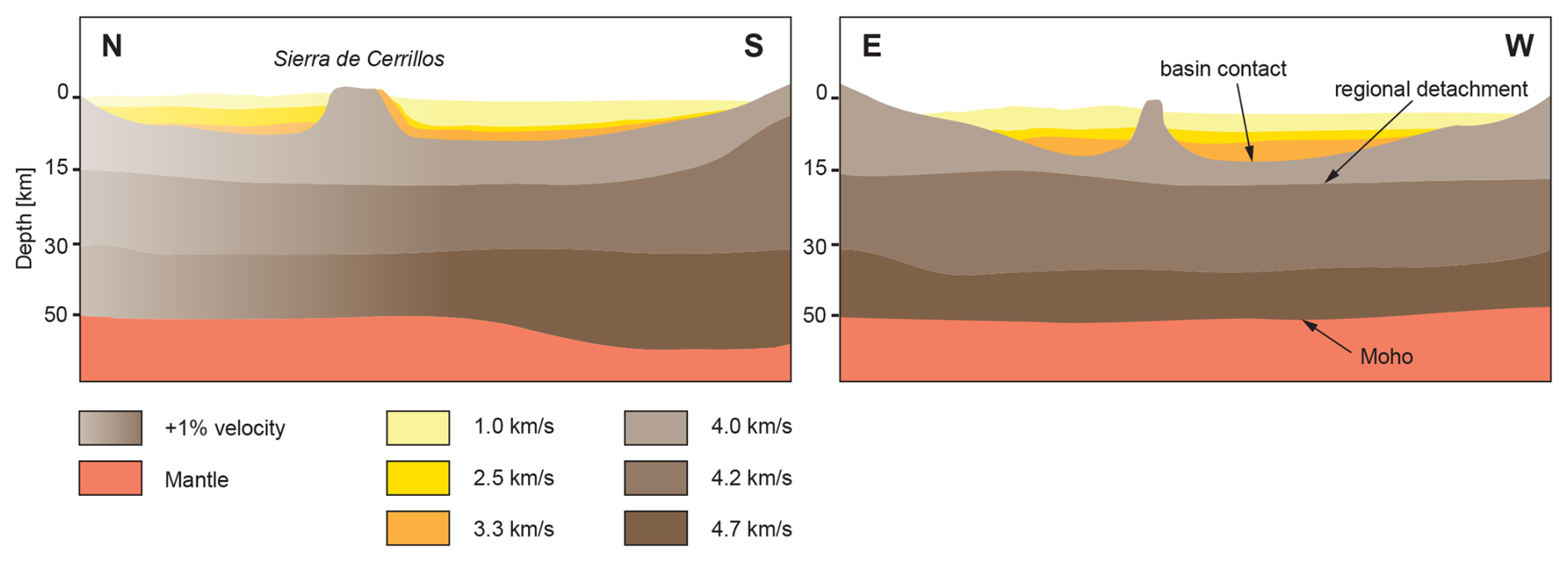
Figure 10 North–south and east–west model profiles of the Lerma Valley, showing four main discontinuities; from the Moho up to the Basin's bedrock contact. Three lesser discontinuities within the Basin. All layers with velocities retrieved form the inversions.

5.11 Shallow Structure and Seismic Hazard Implications

In addition, it should be noted that the upper layers of the model mentioned above, down to five kilometers, include a low velocity layer of about 0.7 km s⁻¹. This feature can be attributed to the Tajamar Formation, for the southern stations only (see Sect. 2). The extent of this unit will be relevant, since it is conformed by fine-grained limos that are expected to suffer liquefaction when water oversaturates during strong motion produced by high magnitude events (Elías et al., 2022).

5.12 Regional and Global Context

To further support the interpretation of the main discontinuities identified in this study, it is useful to place them within a broader geophysical context. Crustal interfaces at depths of $\sim \mathrm{40}-\mathrm{50}\mathrm{km}$, interpreted as the Moho, have been consistently documented across the central Andes using a variety of seismic techniques, including receiver functions, refraction profiles, and gravity-constrained models (Zandt et al., 1996; Yuan et al., 2002; Beck et al., 2015). Similarly, mid-crustal discontinuities near $\sim \mathrm{25}-\mathrm{35}\mathrm{km}$ depth have been widely reported and are often associated with rheological transitions, changes in crustal composition, or zones of partial melt and fluid accumulation (Wigger et al., 1994; Schurr et al., 2006). Shallower discontinuities, particularly those located between ∼10 and 20 km depth, are frequently interpreted as detachment horizons or zones of mechanical decoupling within orogenic crust, reflecting complex deformation processes and strain partitioning (Allmendinger et al., 1997; Yuan et al., 2000). The depths and characteristics of the discontinuities observed in this study are therefore consistent with first-order crustal structures reported throughout the Andean system.

In addition to regional-scale observations, similar multi-layered crustal architectures have been identified in other tectonically active regions worldwide, reinforcing the interpretation of the observed interfaces. For instance, studies in the Tibetan Plateau and other continental collision zones reveal comparable patterns of Moho topography, mid-crustal layering, and upper crustal detachments, often linked to crustal shortening, underplating, and channel flow processes (Nábelek et al., 2009). In these settings, variations in seismic velocity across discontinuities are not uniquely indicative of tectonic boundaries but may also reflect changes in lithology, anisotropy, temperature, or fluid content (Christensen, 1996; Hacker et al., 2003). This highlights the importance of integrating multiple geophysical constraints, as done in this study, to reduce ambiguity and provide a more robust interpretation of crustal structure.

5.13 Integrated Structural Model

The final Fig. 10 provides a synthetic summary of the structures inferred from this study, integrating all results into two lithospheric-scale profiles across the Lerma Valley. One profile is oriented north–south and the other east–west, allowing the three-dimensional geometry of the subsurface to be visualized through two orthogonal sections. These profiles combine constraints from receiver functions, H−κ stacking, and inversion-derived velocity models into a unified structural framework. The principal seismic discontinuities are explicitly traced, illustrating variations in crustal thickness and the geometry of deeper interfaces across the study area.

Seismic velocities are indicated along both sections, and the main velocity gradients are emphasized to highlight vertical and lateral heterogeneities within the crust and upper mantle. The comparison between the north–south and east–west profiles reveals structural asymmetries and along-strike variations that are not evident in individual station-based results alone. By condensing the dataset into these two orthogonal cross-sections, the figure provides an integrated view of the lithospheric architecture beneath the Lerma Valley and serves as a structural reference for the geodynamic interpretation discussed above.

6 Conclusions

In conclusion, the results of this study provide a detailed and coherent image of the crustal structure beneath the Lerma Valley, derived from the analysis of both local and teleseismic receiver functions in conjunction with surface wave dispersion data. The observed crustal stratification is broadly consistent with previous models proposed by Zeckra (2020) and Cahill et al. (1992), particularly in the agreement of the upper layers with the known sedimentary basin structure, characterized by low velocities reaching down to 2.5 km s⁻¹.

The structural interpretation revealed four major discontinuities at approximate depths of 53–43, 35–30, 10–8, and 1.5–1.2 km. These are clearly imaged in the migrated receiver function stacks and supported by the CCP analysis. The deepest discontinuity corresponds to the Moho, which exhibits a southward-dipping geometry as observed in the L-component of the teleseismic RFs. The second interface marks the transition between the lower and middle crust, while the third delineates the upper limit of a possible detachment zone. The shallowest interface defines the basement of the sedimentary basin.

Importantly, the Common Conversion Point (CCP) migration (see Fig. 8) reconfirms a pronounced north–south contrast in crustal architecture. In the north–south profile ($A-A^{\prime }$), the Moho and intermediate discontinuities appear sharper and better defined, particularly in the local receiver functions, with a clear deepening of the Moho towards the south–reaching depths greater than 50 km. Additionally, a detachment zone at ∼15 km depth is only evident in the local RFs, suggesting a mid-crustal feature that may be tectonically significant, in terms of stress transfer to the upper layers of the basin.

This north–south differentiation is further supported by the internal velocity variations observed across the valley, ranging from 1–3.5 km s⁻¹. The southern sector is characterized by lower velocities, likely reflecting less consolidated sedimentary sequences, while the northern sector presents higher velocities associated with more competent crustal material.

The velocity model resulting from the joint inversion of receiver functions and Rayleigh wave phase velocities is robust and well-constrained. It comprises five distinct layers: (1) a soft upper sediment layer (0.8 km thick, 1.25 km s⁻¹), (2) a medium-consolidated sediment layer (3.7 km, 2.83 km s⁻¹), (3) a lower consolidated sediment layer (2 km, 3.25 km s⁻¹), (4) a middle crustal layer (32 km, 3.9 km s⁻¹), and (5) a lower crustal layer (10 km, 4.1 km s⁻¹). These results provide key insights into the crustal architecture and geodynamic context of the Lerma Valley and establish a valuable reference for future seismic and tectonic investigations in the region.

Appendix A: Bottom-Up Recursive Correction of Layered $v_p/v_s$ Ratios

A1 Weighted-Average Forward Model

For a stack of n horizontal layers, the effective or measured ratio $k_{\text{meas},i}^{\left(n\right)}$ inferred from receiver-function H−k analysis at depth index i is given by the weighted average

$$\begin{array}{}\text{(A1)}& k_{\text{meas},i}^{\left(n\right)}={\displaystyle \frac{{\sum }_{j=i}^n{k}_j{v}_{p,j}{H}_j}{{\sum }_{j=i}^n{v}_{p,j}{H}_j}},\end{array}$$

where H_j is the layer thickness, v_p,j the P-wave velocity, and $k_j=v_{p,j}/v_{s,j}$ the intrinsic ratio of the jth layer. This relation expresses the measured value as a cumulative weighted mean over all layers above the conversion depth of interest.

Define the cumulative weight

$$\begin{array}{}\text{(A2)}& N_i=\sum _{j=i}^n{v}_{p,j}{H}_j,w_j=v_{p,j}{H}_j,\end{array}$$

so that Eq. (A1) can be written

$$\begin{array}{}\text{(A3)}& k_{\text{meas},i}^{\left(n\right)}{N}_i=\sum _{j=i}^n{k}_j{w}_j.\end{array}$$

A2 Derivation of the Bottom-Up Recursive Relation

Consider the expression above evaluated at i and i+1:

$$\begin{array}{}\text{(A4)}& {\displaystyle }{k}_{\text{meas},i}^{\left(n\right)}{N}_i& {\displaystyle }=k_i{w}_i+\sum _{j=i+\mathrm{1}}^n{k}_j{w}_j,\text{(A5)}& {\displaystyle }{k}_{\text{meas},i+\mathrm{1}}^{\left(n\right)}{N}_{i+\mathrm{1}}& {\displaystyle }=\sum _{j=i+\mathrm{1}}^n{k}_j{w}_j.\end{array}$$

Subtracting the two equations and solving for k_i yields the bottom-up recursive formula:

$$\begin{array}{}\text{(A6)}& k_i={\displaystyle \frac{k_{\text{meas},i}^{\left(n\right)}{N}_i-k_{\text{meas},i+\mathrm{1}}^{\left(n\right)}{N}_{i+\mathrm{1}}}{w_i}}.\end{array}$$

This expression shows that the estimate of k_i depends only on the cumulative measurements at depths i and i+1 and the local weight w_i.

A3 Matrix Representation

The system can be expressed compactly in linear-algebra form. Let

$$\mathit{k}=\left[\begin{array}{c}{k}_{\mathrm{1}}\\ k_{\mathrm{2}}\\ \mathrm{⋮}\\ k_n\end{array}\right],\mathit{N}=\left[\begin{array}{c}{N}_{\mathrm{1}}\\ N_{\mathrm{2}}\\ \mathrm{⋮}\\ N_n\end{array}\right],$$

and define the upper-triangular cumulative-weight matrix

$$\mathit{L}=\left[\begin{array}{ccccc}{w}_{\mathrm{1}}& w_{\mathrm{2}}& w_{\mathrm{3}}& \mathrm{\cdots }& w_n\\ \mathrm{0}& w_{\mathrm{2}}& w_{\mathrm{3}}& \mathrm{\cdots }& w_n\\ \mathrm{0}& \mathrm{0}& w_{\mathrm{3}}& \mathrm{\cdots }& w_n\\ \mathrm{⋮}& \mathrm{⋮}& \mathrm{⋮}& \mathrm{\ddots }& \mathrm{⋮}\\ \mathrm{0}& \mathrm{0}& \mathrm{0}& \mathrm{\cdots }& w_n\end{array}\right],$$

so the forward model reads

$$\begin{array}{}\text{(A7)}& \mathit{L}\mathit{k}=\mathit{N}.\end{array}$$

The inverse system, obtained by solving this triangular matrix, is

$$\begin{array}{rl}{\displaystyle }\mathit{k}& {\displaystyle }={\mathit{L}}^{-\mathrm{1}}\mathit{N}\\ {\displaystyle }& {\displaystyle }=\left[\begin{array}{ccccc}\mathrm{1}/w_{\mathrm{1}}& -\mathrm{1}/w_{\mathrm{1}}& \mathrm{0}& \mathrm{\cdots }& \mathrm{0}\\ \mathrm{0}& \mathrm{1}/w_{\mathrm{2}}& -\mathrm{1}/w_{\mathrm{2}}& \mathrm{\cdots }& \mathrm{0}\\ \mathrm{0}& \mathrm{0}& \mathrm{1}/w_{\mathrm{3}}& \mathrm{\cdots }& \mathrm{0}\\ \mathrm{⋮}& \mathrm{⋮}& \mathrm{⋮}& \mathrm{\ddots }& \mathrm{⋮}\\ \mathrm{0}& \mathrm{0}& \mathrm{0}& \mathrm{\cdots }& \mathrm{1}/w_n\end{array}\right]\mathit{N}.\end{array}$$

Hence, componentwise,

$$\begin{array}{}\text{(A8)}& k_n={\displaystyle \frac{N_n}{w_n}},k_i={\displaystyle \frac{N_i-N_{i+\mathrm{1}}}{w_i}},i=\mathrm{1},\mathrm{\dots },n-\mathrm{1},\end{array}$$

which is equivalent to the recursive solution (A6).

A4 Error Propagation and Stability

For small measurement uncertainties, standard error propagation yields

$$\begin{array}{}\text{(A9)}& {\mathit{\sigma }}_{k_i}^{\mathrm{2}}={\displaystyle \frac{{\mathit{\sigma }}_{N_i}^{\mathrm{2}}+{\mathit{\sigma }}_{N_{i+\mathrm{1}}}^{\mathrm{2}}}{w_i^{\mathrm{2}}}}.\end{array}$$

Because only two adjacent cumulative terms contribute, uncertainties grow linearly with depth and the system remains well-conditioned. The recursion is anchored at the deepest layer (where the H−k stacking is generally most reliable), making the bottom-up approach intrinsically more stable.

By contrast, the top-down recursion,

$$\begin{array}{}\text{(A10)}& k_i={\displaystyle \frac{k_{\text{meas}}^{\left(i\right)}{\sum }_{j=\mathrm{1}}^n{w}_j-{\sum }_{j=\mathrm{1}}^{i-\mathrm{1}}{k}_j{w}_j}{w_i}},\end{array}$$

introduces all upper-layer uncertainties into the deeper estimates, causing error amplification with depth. This makes top-down inversion less suitable for constraining lower-crustal or Moho properties.

A5 Instability of the Correction in Thin Upper Layers

To illustrate inherent limitations, consider a two-layer system. Rearranging Eq. (A1) at i=1 gives

$$\begin{array}{}\text{(A11)}& k_{\mathrm{1}}={\displaystyle \frac{k_{\text{meas},\mathrm{1}}(v_{p,\mathrm{1}}{H}_{\mathrm{1}}+v_{p,\mathrm{2}}{H}_{\mathrm{2}})-k_{\text{meas},\mathrm{2}}{v}_{p,\mathrm{2}}{H}_{\mathrm{2}}}{v_{p,\mathrm{1}}{H}_{\mathrm{1}}}}.\end{array}$$

When v_p,1H₁ is small (thin sediments or low v_p,1), the denominator becomes small and the estimate of k₁ becomes highly sensitive to uncertainties in the measured or assumed deeper-layer values.

The sensitivity to measurement uncertainty is

$$\begin{array}{}\text{(A12)}& {\displaystyle \frac{\partial k_{\mathrm{1}}}{\partial k_{\text{meas},\mathrm{1}}}}=\mathrm{1}+{\displaystyle \frac{v_{p,\mathrm{2}}{H}_{\mathrm{2}}}{v_{p,\mathrm{1}}{H}_{\mathrm{1}}}},\end{array}$$

which becomes large as $v_{p,\mathrm{1}}{H}_{\mathrm{1}}\to \mathrm{0}$. Thus, shallow layers cannot be reliably corrected unless their P-wave velocity and thickness are well constrained.

A6 Generalization to Arbitrary Incidence Angle

For a general ray parameter (or incidence angle), the forward model ceases to be linear. Following the standard moveout expressions, the effective ratio becomes

$$\begin{array}{}\text{(A13)}& k_{\text{meas}}^{\left(j\right)}={\displaystyle \frac{{\sum }_{i=\mathrm{1}}^j{v}_{p,i}\sqrt{k_i^{\mathrm{2}}-{\sin }^{\mathrm{2}}{\mathit{\alpha }}_i}{H}_i}{{\sum }_{i=\mathrm{1}}^j{v}_{p,i}\left|\cos {\mathit{\alpha }}_i\right|H_i}},\end{array}$$

where α_i is the incidence angle within layer i. Because the numerator includes $\sqrt{k_i^{\mathrm{2}}-{\sin }^{\mathrm{2}}{\mathit{\alpha }}_i}$ while the denominator depends on $\left|\cos {\mathit{\alpha }}_i\right|$, the expression is strongly nonlinear in both k_i and α_i.

A7 Comparison of Bottom-Up and Top-Down Approaches

The bottom-up method inherits stability from its triangular structure: each k_i depends only on the cumulative weights at depths i and i+1 and the local weight w_i. Errors accumulate slowly and remain bounded with increasing depth.

The top-down (head-down) method, in contrast, uses successively more cumulative quantities from all above layers, causing uncertainties to compound. Deep layers – which are often the most geophysically important – receive the worst error amplification.

Empirical evaluations confirm this behavior: bottom-up estimates of lower-crustal and Moho k values have consistently smaller uncertainties.

A8 Relation to Pseudo-Wadati Estimates

The classical Wadati relation,

$$\begin{array}{}\text{(A14)}& T_s^{\left(j\right)}=k_{\text{Wadati}}{T}_p^{\left(j\right)}+{\mathit{\epsilon }}_j,\end{array}$$

yields an apparent crustal $v_p/v_s$ ratio via regression. Layerwise decomposition of the P- and S-travel times shows

$$\begin{array}{}\text{(A15)}& {\widehat{k}}_{\text{Wadati}}={\displaystyle \frac{{\sum }_i{k}_i{w}_i}{{\sum }_i{w}_i}},w_i=\sum _j{\mathit{\beta }}_i^{\left(j\right)}{T}_p^{\left(j\right)},\end{array}$$

so the regression slope is a weighted mean of the true k_i values. Because deep layers contribute most strongly to the travel-time budget, Wadati estimates naturally tend to reflect the lower-crust or Moho ratio. This behavior is consistent with the stability of the bottom-up recursive correction, which likewise anchors its solution at the deepest layer.

A9 Summary

The bottom-up recursive correction provides a robust and well-conditioned method for estimating layerwise $v_p/v_s$ ratios from cumulative receiver-function measurements. Its triangular algebraic structure limits uncertainty growth and makes it particularly well suited for constraining lower-crustal and Moho properties. Upper-layer estimates, however, remain subject to strong instability if the shallow P-wave velocity or thickness is poorly constrained. Generalization to arbitrary incidence angles introduces strong nonlinearity and does not yield a comparable linear inversion scheme.

Appendix B: Empirical tests for the selection of forward-modeling parameters

The forward-modeling and preprocessing parameters adopted in this study were selected on the basis of empirical tests aimed at identifying a configuration that provides an improved fit to the observed receiver functions. Rather than performing a formal sensitivity analysis, we evaluated the effect of moderate variations in the main processing parameters on the quality of the forward modeling results.

Starting from a reference configuration, each parameter was varied independently by approximately ±10 %, while all other settings were kept fixed. The parameters tested include the Gaussian filter coefficients a and c, the sampling interval dt, the ray parameter p, and the maximum depth L. For each tested configuration, synthetic receiver functions were computed and visually and quantitatively compared with the observed data.

These tests showed that the parameter set adopted in the main text (a=1.5, c=0.001, dt=0.1 s, $p=\mathrm{0.045}\mathrm{s}/\mathrm{°}$, and $L=\mathrm{0}-\mathrm{50}\mathrm{km}$) consistently produced a better agreement between observed and synthetic receiver functions than the alternative configurations explored. In particular, departures from this configuration either led to increased waveform misfit or to less stable and noisier synthetic receiver functions.

On this basis, the selected parameter values were retained for all inversions presented in this study, as they represent an empirically determined setup that optimizes the quality of the receiver-function fit within the range of tested parameter variations.