the Creative Commons Attribution 4.0 License.
the Creative Commons Attribution 4.0 License.
 | 11 Jan 2019
A semi-automated algorithm to quantify scarp morphology (SPARTA): application to normal faults in southern Malawi
Juliet Biggs
Åke Fagereng
Austin Elliott
Hassan Mdala
Felix Mphepo
Along-strike variation in scarp morphology reflects differences in a fault's geomorphic and structural development and can thus indicate fault rupture history and mechanical segmentation. Parameters that define scarp morphology (height, width, slope) are typically measured or calculated manually. The time-consuming manual approach reduces the density and objectivity of measurements and can lead to oversight of small-scale morphological variations that occur at a resolution impractical to capture. Furthermore, inconsistencies in the manual approach may also lead to unknown discrepancies and uncertainties between, and also within, individual fault scarp studies. Here, we aim to improve the efficiency, transparency and uniformity of calculating scarp morphological parameters by developing a semi-automated Scarp PARameTer Algorithm (SPARTA). We compare our findings against a traditional, manual analysis and assess the performance of the algorithm using a range of digital elevation model (DEM) resolutions. We then apply our new algorithm to a 12 m resolution TanDEM-X DEM for four southern Malawi fault scarps, located at the southern end of the East African Rift system: the Bilila–Mtakataka fault (BMF) and three previously unreported scarps – Thyolo, Muona and Malombe. All but Muona exhibit first-order structural segmentation at their surface. By using a 5 m resolution DEM derived from high-resolution (50 cm pixel−1) Pleiades stereo-satellite imagery for the Bilila–Mtakataka fault scarp, we quantify secondary structural segmentation. Our scarp height calculations from all four fault scarps suggest that if each scarp was formed by a single, complete rupture, the slip–length ratio for each earthquake exceeds the maximum typical value observed in historical normal faulting earthquakes around the world. The high slip–length ratios therefore imply that the Malawi fault scarps likely formed in multiple earthquakes. The scarp height distribution implies the structural segments of both the BMF and Thyolo fault have merged via rupture of discrete faults (hard links) through several earthquake cycles, and the segments of the Malombe fault have connected via distributed deformation zones (soft links). For all faults studied here, the length of earthquake ruptures may therefore exceed the length of each segment. Thus, our findings shed new light on the seismic hazard in southern Malawi, indicating evidence for a number of large (Mw 7–8) prehistoric earthquakes, as well as providing a new semi-automated methodology (SPARTA) for calculating scarp morphological parameters, which can be used on other fault scarps to infer structural development.
- Article
(9720 KB) - Full-text XML
-
Supplement
(5351 KB) - BibTeX
- EndNote


Earthquake ruptures that break the Earth's surface result in the offset of landforms such as river channels, alluvial fans and other geomorphic features (Hetzel et al., 2002; Zhang and Thurber, 2003), and create fault scarps that are themselves indicative of the style and magnitude of the earthquake event (Wallace, 1977). The scarps may be formed by a single earthquake or a small number of events, or represent the cumulative effect of numerous events over geological timescales. Linking the surface offset along the fault to information on the age of the features can provide information about the rupture and slip history on the fault (Ren et al., 2016; Sieh, 1978; Wallace, 1968; Zielke et al., 2012). For mature faults, it can be used to characterise long-term development by identifying structural segmentation (Giba et al., 2012; Manighetti et al., 2015; Watterson, 1986) and the presence of linking structures (Nicol et al., 2010; Soliva and Benedicto, 2004). For faults whose component segments remain unconnected at the surface, the distribution of displacement along a fault can also provide clues to the future structural development (Cowie and Scholz, 1992; Dawers and Anders, 1995; Dawers et al., 1993; Peacock, 2002; Walsh and Watterson, 1988) by indicating soft linkages between segments (Hilley et al., 2001; Willemse et al., 1996), such as relay ramps. Over time, these segments may hard link; i.e. a connection establishes between segments via rupture of discrete fault planes (Childs et al., 2017; Hodge et al., 2018b). Thus, using a combination of the displacement distribution along a fault and the inter-segment zone geometry, we can understand what linkage might exist at depth (Crider and Pollard, 1998). The importance of distinguishing between these two types of linkages is that the physical connection of a hard link may permit through-going earthquake rupture and will also increase fluid transport, with implications for reservoirs.
In the past, calculating the displacement across a fault scarp was performed by local field surveys or using Global Positioning System (GPS) devices (e.g. Andrews and Hanks, 1985; Avouac, 1993; Bucknam and Anderson, 1979; Cartwright et al., 1995; Cowie and Scholz, 1992; Delvaux et al., 2012; Gillespie et al., 1992). However, recent advances in remote sensing have meant that highly accurate and precise vertical displacements can be measured using satellite images and digital elevation models (DEMs) (e.g. Westoby et al., 2012, Bemis et al., 2014, Johri et al., 2014, Zhou et al., 2015, Roux-mallouf et al., 2016, Talebian et al., 2016). Depending on resolution, DEMs are categorised as low (≥30 m), intermediate (∼10 m) or high resolution (≤5 m). There is a trade-off between DEM resolution and cost as launching satellites and acquiring (tasking) images is expensive. High-resolution DEMs generated by the newest satellites are expensive, exacerbated by large minimum coverage areas (typically ∼100 km2). Furthermore, generating a DEM using high-resolution satellite images may require preprocessing steps including pan sharpening and stereo-alignment. As a satellite programme becomes discontinued, satellite images and DEMs are often released for scientific use at no cost (e.g. the SPOT Historical archive, Shuttle Radar Topography Mission). These products require limited to no post-processing. Nonetheless, even relatively high-resolution stereo-image derived DEMs have vertical uncertainties, or noise, amounting to around ≥30 cm (Zhou et al., 2015), controlling the minimum scale of geomorphic features that can be confidently detected.
With the current drive toward acquisition of high-resolution DEMs for paleoseismological studies (e.g. Zhou et al., 2015; Roux-mallouf et al., 2016; Talebian et al., 2016), two scientific questions arise: (1) what DEM resolution is required to successfully locate, calculate and accurately analyse significant changes in displacement along a fault scarp; and (2) does our interpretation of the distribution of displacement scale with DEM resolution (i.e. how much more are we able to infer using an expensive, high-resolution DEM compared to a free, lower-resolution alternative)?
Despite the advances in satellite and computing technology, and thus the resolution of DEMs, calculating the vertical displacement along a scarp is largely a manual process that has remained consistent over several decades (Avouac, 1993; Bucknam and Anderson, 1979; Ganas et al., 2005; Walker et al., 2015; Wallace, 1977; Wu and Bruhn, 1994). Scarp height is typically used as a proxy for minimum vertical displacement (Morewood and Roberts, 2001). Scarp height is typically determined by identifying the fault scarp from an elevation profile, fitting lines to slopes that are on either side of the scarp and measuring the offset between these fitted lines. However, picking the fault scarp location manually can be unrepeatable for intermediate- or low-resolution DEMs, with measurements showing variability in picked scarp location for multiple independent analyses on the same profiles (Hodge et al., 2018a). Manually processing data can also be subject to human bias; one person's definition of the crest and base of a fault scarp may be different from another person's (Middleton et al., 2016). These inconsistencies ultimately lead to errors within the scarp height calculations and are a contributing factor for the scatter observed in global maximum displacement-length profiles (Gillespie et al., 1992) and along-strike displacement profiles (Zielke et al., 2015).
In this paper, we develop an algorithm that calculates the parameters (height, width and slope) of a fault scarp from a scarp elevation profile: Scarp PARameTer Algorithm (SPARTA). Using the scarp height as a proxy for vertical displacement (Morewood and Roberts, 2001), a displacement profile can be created by calculating scarp height at intervals along a fault scarp. This displacement profile can then be used to infer fault structural segmentation and the existence of secondary linking faults (Cartwright et al., 1995; Childs et al., 1996; Crone and Haller, 1991; Dawers and Anders, 1995; Giba et al., 2012). Automating the morphological calculations will allow a greater number of measurements to be taken along a fault scarp than feasible with ground based methods, improving the understanding of fault behaviour and segmentation (Cartwright et al., 1995; Manighetti et al., 2015; Trudgill and Cartwright, 1994; Zielke et al., 2012, 2015). Our goal is to develop an algorithm that is open-source and able to run on a personal computer. We test the performance of the algorithm using a number of synthetic and real fault scarps, for a variety of DEM resolutions.
Algorithms for relative dating of fault scarps, by performing best-fit calculations to a scarp-like template, have already been attempted (Gallant and Hutchinson, 1997; Hilley et al., 2010; Stewart et al., 2017); however, these methods may falsely identify other geomorphic features as fault scarps and require a very high-resolution DEM, usually obtained using lidar. These autonomous algorithms therefore still require post-processing, manual quality checks. In addition, Shaw and Lin (1993) developed an algorithm to identify fault scarps by measuring topographic curvature within a moving window; however, their method only distinguishes between different relative scarp heights rather than provides a quantitative measurement of scarp height. The algorithm created here (SPARTA) will be developed to be used for a range of DEM resolutions, where the performance between resolutions is tested in this study.
Our aim is to develop an algorithm capable of measuring along-strike variations in the height of fault scarps at high resolution across a range of settings. The nature of the subsequent analysis and interpretation will, however, depend on the age and type of fault considered as well as the local lithological and climatic conditions. Individual earthquakes can produce scarps of variable height and a mix of on-fault and off-fault deformation (Gold et al., 2015; Milliner et al., 2016; Nissen et al., 2016; Wang et al., 2014). In some circumstances, ruptures are halted by discontinuities or steps in a fault system, whereas other earthquakes produce complex rupture patterns which include multiple fault segments (Hamling et al., 2017; Jackson et al., 1982). Between earthquakes, erosion depends on variations in lithological and climatic properties, which can produce dramatic changes in scarp height over short distances in only a few decades. For example, some parts of the scarp formed in the 1981 Alkyonides earthquake, Gulf of Corinth, are well preserved but others have nearly disappeared (Mechernich et al., 2018). Some fault scarps are formed by individual earthquakes, others are multi-scarps produced by a few events, while others represent the cumulative effects of numerous earthquake cycles over tens of thousands of years. In these cases, variations in scarp height may contain information on fault evolution that can be extracted by identifying structural segmentation (Giba et al., 2012; Manighetti et al., 2015; Watterson, 1986) and the presence of linking structures (Nicol et al., 2010; Soliva and Benedicto, 2004). However, these long-term effects will be convolved with variations associated with individual earthquakes. This combination of timescales involved in scarp generation raises the question as to what extent variations in offset and erosion persist across multiple earthquake cycles.
1.1 Normal faults in southern Malawi
The Malawi Rift system (MRS) exists at the southern end of the East African Rift system (EARS), extending 900 km from the Rungwe province in the north to the Urema Graben in the south (Ebinger et al., 1987; Specht and Rosendahl, 1989). At the northern end of the rift system is the Mbeya box, which is a triple junction between the Somalia, Victoria and Rovuma plates (Ebinger et al., 1989). Rift development commenced around approximately 8 Ma (Ebinger et al., 1989) with the formation of half-graben units bounded by fairly north–south-striking normal faults and propagated from the north (Ring et al., 1992). Kinematic models of plate motion suggest maximum average extension rates across the Malawi Rift of ∼3 mm per year, decreasing southwards to less than 2 mm per year (Jackson and Blenkinsop, 1997; Jestin et al., 1994; Saria et al., 2014; Stamps et al., 2008). Border fault systems exist with a predominantly north–south trend at the edges of Lake Malawi and alternate sides of the lake at around 100 km intervals (Ebinger et al., 1987; Rosendahl et al., 1986).
In the southern MRS, the Bilila–Mtakataka fault (BMF) scarp breaks the surface along almost its entire length, a distance of ∼ 110 km (Hodge et al., 2018a; Jackson and Blenkinsop, 1997). Early studies suggested that the scarp formed during a single earthquake (Jackson and Blenkinsop, 1997), but the morphology and geometry vary along strike (Hodge et al., 2018a) and are more typical of a large, structurally segmented normal fault which has experienced several previous earthquake cycles (Peacock and Sanderson, 1991; Schwartz and Coppersmith, 1984; Wesnousky, 1986). The fault is suggested to comprise six major (first-order) segments, varying in length from 13 to 38 km, and the distribution of scarp height is of two symmetrical bell-shaped profiles separated by the Citsulo segment (Hodge et al., 2018a). The relatively coarse measurement resolution of the former studies along the BMF have meant that secondary (second-order) segments were unable to be identified or characterised, i.e. subordinate segments that have a length of the same order of magnitude as the major segment they exist within (Manighetti et al., 2015). Although secondary segments are unlikely to contain gaps of sufficient distance (typically inferred to be ≥ 6 km) to perturb rupture propagation (Biasi and Wesnousky, 2016; Gupta and Scholz, 2000), their existence may provide evidence for the earliest structural development of the fault (Manighetti et al., 2007). Furthermore, understanding structural segmentation is crucial in estimating earthquake magnitude, as fault segments may rupture individually, consecutively or continuously (Anderson et al., 2017; Hodge et al., 2015).
The latest morphological analysis also concludes that there may be a gap in the BMF scarp across the Citsulo segment (Hodge et al., 2018a). This discontinuity extends for a maximum length of ∼ 10 km. A break in continuity of this length may be sufficient to perturb rupture propagation (Biasi and Wesnousky, 2016) and prevent hard linkage along a normal fault (Hodge et al., 2018b). A reduced maximum rupture length would reduce the maximum expected earthquake magnitude (Wells and Coppersmith, 1994) and also the earthquake repeat time (Hodge et al., 2015). Therefore, in order to conclude whether the fault scarp is discontinuous across the Citsulo segment, and the existence of secondary segments and associated linking faults, a higher-resolution DEM and a greater number of scarp profiles are required.
Although the Bilila–Mtakataka fault provides an ideal case study of a large, continental normal fault, in order to understand whether it is unique or representative of early stage rift faulting, we extend our research to other fault scarps within the southern, amagmatic MRS. We investigate three additional faults in the southern MRS identified during fieldwork, which have previously unreported scarps: the Malombe, Thyolo and Muona faults. The Malombe fault is a north–south-striking, east-dipping normal fault located ∼ 40 km east of the Bilila–Mtakataka fault, on the edge of Lake Malombe; the fault scarp contains at least two major gaps in its surface expression (Fig. 1c). Lithology varies considerably along the fault length, alternating between felsic and mafic paragneisses with fingers of calc-silicate granulite that intersect the scarp (Manyozo et al., 1972). The Thyolo and Muona faults, south of the Bilila–Mtakataka fault, are two overlapping northwest–southeast-striking, southwest-dipping parallel normal fault scarps separated by an offset of ∼ 5 km (Fig. 1d). The lithology of the scarp footwall is very homogeneous at the regional scale, mapped as mafic paragneiss along its entire length (Habgood et al., 1973). Whereas the Bilila–Mtakataka, Muona and Thyolo faults all lie in the footwall of a major escarpment at the rift border, the Malombe fault is situated near the centre of the rift basin (Fig. 1a). There is no age control on recent earthquakes on any of these faults, neither are the ages of the escarpments known. To infer the distribution of scarp height, structural segmentation and linkage structures along the Malombe, Thyolo and Muona fault scarps, we develop an algorithm to calculate profiles of the height and width of the scarp. We then compare our findings for these newly studied faults with the Bilila–Mtakataka fault and assess their morphology and structural development. We also calculate the slip–length ratio for each fault and compare against previously observed values for normal fault earthquakes (Scholz, 2002).
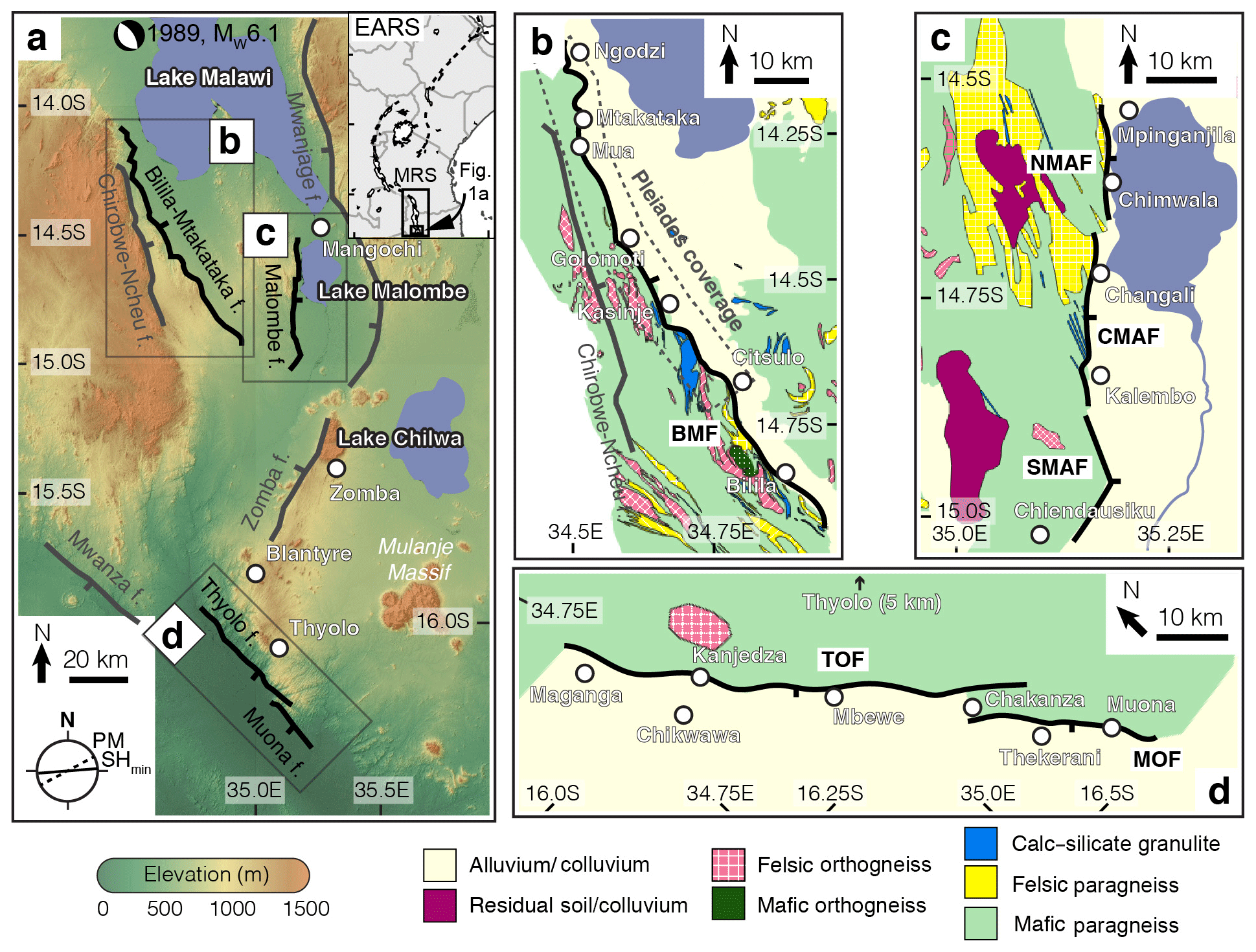
Figure 1(a) Map of faults in southern Malawi; those used in this study are coloured black. Tick marks show the dip direction. Lower left corner shows the plate motion (PM; 86∘ ± 5∘) from Saria et al. (2014) and local minimum horizontal stress (SHmin; 62∘) from Delvaux and Barth (2010). Top right corner shows the location with respect to the East African Rift system (EARS) and Malawi Rift system (MRS). Panels (b)–(d) are geological maps of (b) the Bilila–Mtakataka fault (BMF) showing the coverage of the Pleiades satellite imagery (Dawson and Kirkpatrick, 1968; Walshaw, 1965); (c) the Malombe fault (MAF): northern Malombe fault (NMAF), central Malombe fault (CMAF) and southern Malombe fault (SMAF) (Manyozo et al., 1972); and (d) the Thyolo fault (TOF) and Muona fault (MOF) (Habgood et al., 1973).
2.1 Algorithm development
2.1.1 Scarp identification
For a given profile perpendicular to the local scarp trend, the first step in calculating the scarp's morphological parameters (height, width and slope) is to identify the exact position of the scarp within the data, essentially defined by the scarp crest and base that bound it. Figure 2a–c show three profiles from the Bilila–Mtakataka fault scarp taken using the 5 m DEM derived from 50 cm Pleiades imagery. The black line shows the elevation data extracted from the DEM, the red line shows the change in elevation per unit distance (i.e. slope, θ), and the blue circles are the derivative of slope (ϕ). Each of the three profiles is characteristic of a different challenge associated with picking the fault scarp manually. The quality of the profile is determined by the non-tectonic features present in the DEM. Profile A has a large, wide scarp that is clearly defined with little ambiguity from other topographic features; however, the gradient of the scarp is not constant, leading to large slope derivative values (Fig. 2a). Profile B has an ambiguous scarp morphology, caused by vegetation or other topographical features; these features create local variability in slope θ, yet the gradient of the scarp itself is fairly constant (Fig. 2b). Profile C is clear of other topographic features, the scarp width is small and the magnitude of the change in slope at the fault scarp is not large; it is therefore difficult to accurately identify the scarp from the footwall topography (Fig. 2c). Furthermore, Profile C's morphology makes picking a fault scarp even more challenging when using a lower-resolution DEM.
For each profile in Fig. 2, grey triangles denote a manual pick of the crest and base of the fault scarp. These picks are used to define scarp width. We consider the basic assumption that the fault scarp represents the approximate position of the fault. A linear regression (least-squares method) is then applied to the upper original and lower original surfaces away from the scarp. The best-fitting regression lines for the upper and lower original surfaces (grey dotted lines) are then extrapolated to the point of maximum slope (θmax) on the identified fault scarp (Fig. 3). The scarp height H is then taken as the elevation difference between the regression lines at this point, the gradient of the best-fit line through the fault scarp is the scarp slope α, and the horizontal distance between fault scarp crest and base is the scarp width W.
Our algorithm picks the crest and base of the fault scarp based on the first and last values of the scarp profile that satisfy a priori threshold values of slope (θT) and the derivative of slope (ϕT). For the algorithm to calculate accurate values for scarp height, width and slope, the thresholds need to be appropriate for the scarp's morphology; i.e. for gently dipping fault scarps, the slope threshold should also be of a gentle angle. Two examples for slope threshold are shown for the profiles in Fig. 2: one where the slope threshold is set to 20∘ (pink triangles) and one where it is 40∘ (blue triangles). For all profiles, neither threshold value performs well at automatically identifying a fault scarp equivalent to the one that was determined manually. The reason for the poor algorithm performance is ambiguity in the scarp morphology, where non-tectonic features may lead to the misidentification of the fault scarp by the algorithm. For example, in Fig. 2a and c, the algorithm fails to accurately identify the base of the fault scarp due to irregularities in the lower original surface. For all examples, the crest of the fault scarp is misidentified by the algorithm due to topographic features within the upper original surface. Furthermore, as the values of ϕ have a higher amplitude than θ, the algorithm is more sensitive to the slope derivative threshold than the slope threshold. To enhance the clarity of the elevation profiles, we apply and test a range of digital filters that will essentially remove non-tectonic features from the data.

Figure 2Panels (a) to (c) show three profiles across the Bilila–Mtakataka fault scarp using the Pleiades 5 m DEM. Each is characteristic of the different challenges associated with picking the fault scarp manually and using an algorithm. Profile A has a clearly defined scarp, although the scarp itself contains non-tectonic topographic features making it difficult to quantify its shape. Profiles B and C have more distributed topographic noise, and Profile C has a scarp that is difficult to accurately identify as the magnitude of the change in slope at the fault scarp is not large. Using Profile B, four different digital filters and/or bin widths were applied: (d) Lowess (bin width 20 m); (e) moving mean (bin width 20 m); (f) Savitzky–Golay (bin width 20 m); and (g) Lowess (bin width 40 m). The black line is the elevation profile, the red line is the slope (θ) profile, and blue circles denote the derivative of slope (ϕ). Grey triangles show the location of the crest and base of the fault scarp based on a manual pick. Pink and blue triangles denote the algorithm's pick of the crest and base based on a slope threshold of 20∘ (pink) and 40∘ (blue), respectively.
2.1.2 Filtering
Here, we test the suitability of four digital filters (moving mean, moving median, Savitzky–Golay and Lowess) in smoothing out non-tectonic features in the scarp profiles and improving the accuracy with which morphological parameters such as height and width can be extracted by automated processing. Each filter uses a moving window over a specified bin width, which must be an odd integer. The moving window is incrementally shifted along the profile for each data point.
For the moving mean and moving median filters, we use the rolling mean algorithm from the pandas Python module and the moving median algorithm from the SciPy Python module, respectively. Both filters are commonly used signal-processing algorithms because they are the easiest and fastest digital filters to understand and use. In image processing, the median filter is usually the preferred digital filter to represent an average. This is because an individual unrepresentative value in the window will not affect the median value as significantly as it affects the mean. However, the median filter also preserves sharp edges and therefore may lead to step-like features, which could cause steep slope artefacts in our profiles. The Savitzky–Golay filter is based on a local least-squares polynomial approximation (Savitzky and Golay, 1964); it is less aggressive than simple moving filters and is therefore better at preserving data features such as peak height and width. The Lowess filter uses a non-parametric regression method and requires larger sample sizes than the other filters (Cleveland, 1981). The Lowess filter can be performed iteratively, but since it requires much more computational power than the other filter methods, we apply a single pass over the data.
Figure 2d–g show the results of applying a digital filter to Profile B (Fig. 2b). This profile was chosen because of the extensive topographic variation within the upper original surface. Such irregularity is typical for fault scarp profiles, as topographic features from previous deformation events, valleys and dense vegetation are common. The elevation data were filtered using the following parameters: (d) Lowess (bin width 20 m); (e) moving mean (bin width 20 m); (f) Savitzky–Golay (bin width 20 m); and (g) Lowess (bin width 40 m). Filter parameters for Profiles D, E and F were chosen as a comparison between three different filter methods using the same bin width, whilst parameters for Profiles D and G were chosen for a comparison between different bin widths for the same filter method.
The Lowess and Savitzky–Golay filters smooth the elevation, and subsequently the profiles of slope θ and slope derivative ϕ, more than the moving mean filter. As expected, a larger bin width smooths the data more than a smaller bin width. By smoothing the data, the relative amplitude of ϕ becomes smaller than that of θ, meaning that the algorithm becomes less sensitive to the slope derivative threshold than the slope threshold. For the same bin width (20 m), the algorithm using the Lowess and Savitzky–Golay filters estimates the scarp location more accurately than the moving mean for this profile, as the latter fails to significantly reduce the ambiguity caused by non-tectonic features within the upper original surface; however, for all filters, the algorithm still falsely identifies the crest of the fault scarp using a slope threshold of 20 or 40∘. The algorithm using a slope threshold of 20∘ performs reasonably well once the profile has been filtered using the Lowess filter and a bin width of 40 m (Fig. 2f), for this example.
The Lowess filter smooths the elevation, and subsequently the profiles of slope θ and slope derivative ϕ, more than the moving mean filter. As expected, a larger bin width smooths the data more than a smaller bin width. By smoothing the data, the relative amplitude of ϕ becomes smaller than that of θ, meaning that the algorithm becomes less sensitive to the slope derivative threshold than the slope threshold. For the same bin width (20 m), the algorithm using the Lowess filter estimates the scarp location more accurately than the moving mean for this profile, as the latter fails to significantly reduce the ambiguity caused by non-tectonic features within the upper original surface; however, for both filters, the algorithm still falsely identifies the crest of the fault scarp using a slope threshold of 20 or 40∘. The algorithm, using a slope threshold of 20∘, performs reasonably well once the profile has been filtered using the Lowess filter and a bin width of 40 m (Fig. 2f), for this example.
2.2 Assessing algorithm performance
We assess the performance of our algorithm by testing it on various scarp profiles. Performance is assessed by defining a misfit value for scarp height (Hm), width (Wm) and slope (αm) as the difference between ground-truthed (Hg, Wg, αg) and algorithm-calculated (Hc, Wc, αc) scarp parameters – based on the selected a priori parameters and filter method – for each profile. Misfit values can be positive or negative. This approach relies on the assumption that the ground-truthed value is correct and is the value that we want the algorithm to calculate. One approach, as shown above, is to use a manual analysis to calculate the ground-truthed values. For example, for Profile G the crest and base were both identified by the algorithm within 5 m of the manual pick, leading to a height misfit of less than 1 m, a width misfit of less than 6 m and a slope misfit smaller than 1∘ (Fig. 2g). Another way to test algorithm performance is to generate a synthetic fault scarp profile where the ground-truthed values are the input parameters.
Although the ultimate goal is to design an algorithm to calculate scarp parameters for real fault scarps, the creation of a synthetic catalogue will allow us to robustly test the algorithm, and the relationship between filter and threshold parameters, using a large number of scarp profiles. This would not be feasible using the manual process. Therefore, the algorithm is run iteratively on a number (n) of synthetic profiles, using a range of a priori filter and threshold values. Average height (), width () and slope () misfit values are then calculated using the mean of individual misfit values from the profiles (Eqs. 1 to 3). The total number of profiles where a fault scarp is identified by the algorithm is given as the count C. The total misfit value, ε, is then calculated using Eq. (4); all algorithm runs where the number of fault scarps identified is fewer than 50 % are removed. Although calculating the correct scarp height is the most important element of our algorithm, an equal weight is applied to all scarp parameters because all contribute to how well the scarp is identified. The smallest ε value is then used to denote the best-performing set of filter and threshold parameters.
3.1 Synthetic catalogue
In order to test the possible combinations of filtering, bin sizes, etc. using a Monte Carlo approach, we construct two synthetic catalogues, with and without non-tectonic features causing topographic noise in the DEM, each comprising 1000 fault scarp profiles.
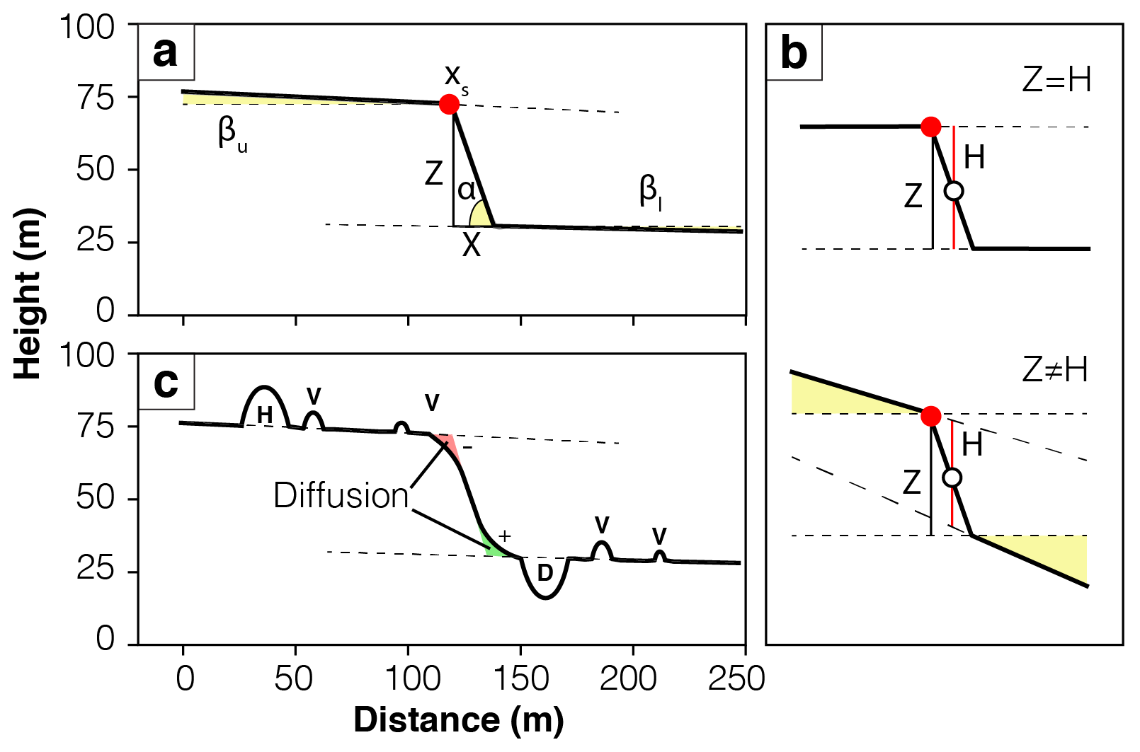
Figure 3An example of a synthetic catalogue fault scarp. (a) Visual description of the parameters in Table 1 used in the synthetic catalogue without non-tectonic features. (b) The difference between vertical displacement Z and synthetic profile scarp height Hg, resulting from sloping original surfaces. (c) The additional non-tectonic synthetic catalogue parameters (H indicates hills; V indicates vegetation; D indicates ditches) and diffusion (red indicates erosion; green indicates deposition).
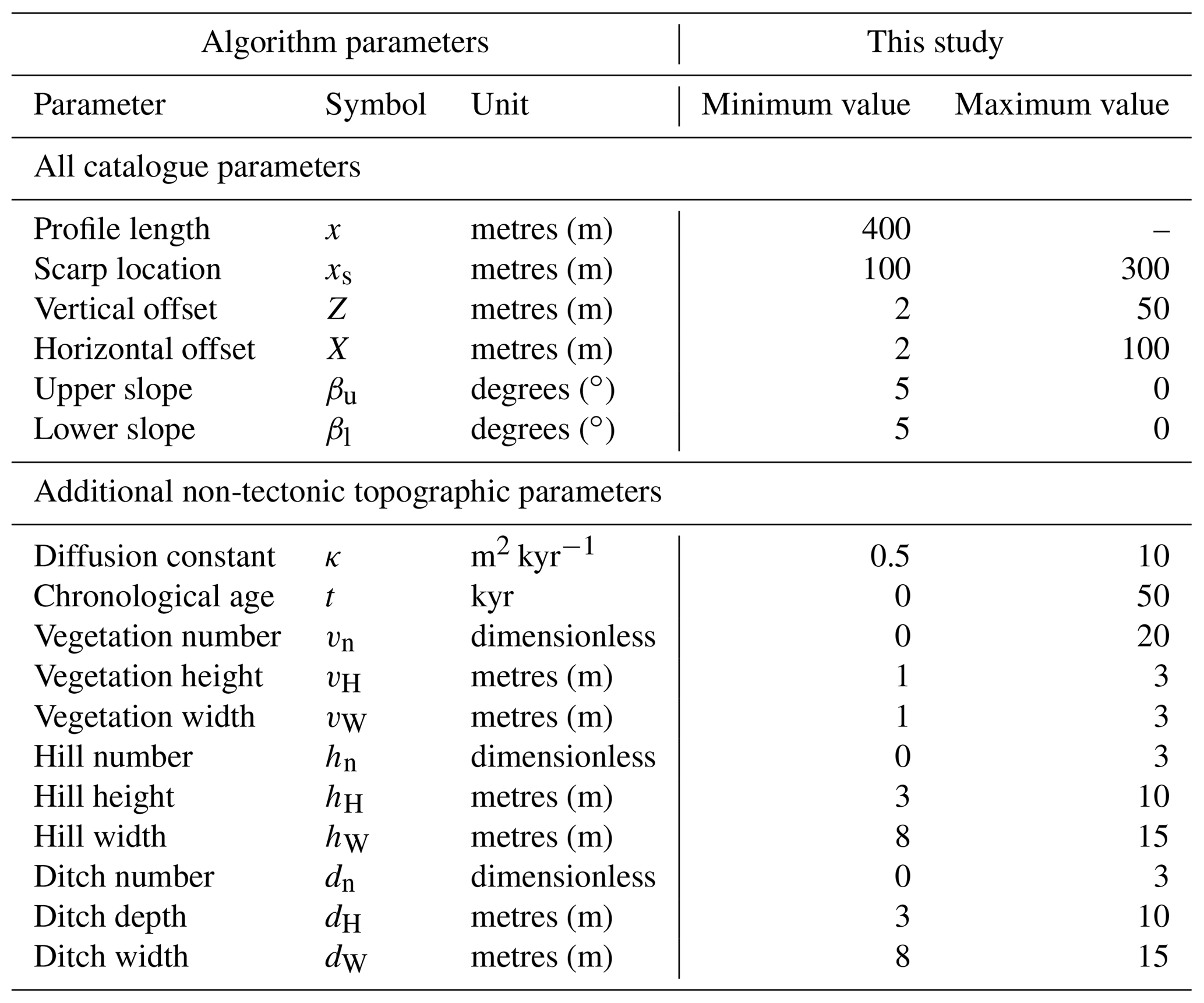
The parameters used in the construction of both catalogues are the location of the scarp crest along the profile (xs), the slope of the upper original surface (βu) and the slope of the lower original surface (βl, Table 1; Fig. 3a). Profile length x and resolution r are constants set to 400 and 1 m, respectively. Parameters βu and βl could be omitted if the synthetic catalogue is used to mimic an environment where fault scarps offset flat surfaces (Ward and Barrientos, 1986) and included for regions where fault scarps offset sloped surfaces (Tucker et al., 2011). A down-dip, normal sense of displacement parallel to the scarp is then imposed, and Z and X are defined as the vertical (throw) and horizontal (heave) components of this displacement. The synthetic fault scarp width Wg therefore equals the horizontal displacement X and scarp slope αg equals . The height of the synthetic fault scarp Hg is then calculated using Eq. (5). The larger the values of βu and βl, the larger the difference between measured throw and actual throw, Hg and Z (Fig. 3b).
The noisy catalogue includes irregularities in the form of non-tectonic topographic features such as vegetation, hills and ditches, as well as scarp degradation by diffusion (Table 1; Fig. 3c). A random number of these non-tectonic features are placed at random locations along the profile. The shape of these features is a negative parabola between a and b, created using Eq. (6), where a is the first root at the random location and b is the second root at a horizontal distance from the first root equating to the feature width, with a height .
Diffusion is applied in a Monte Carlo approach by using Eq. (7) for a diffusion constant κ and time t, resulting in erosion of material from the upper portion of the scarp and deposition at the base (Fig. 3c). Diffusion can be included for environments where hillslopes are mantled with a continuous soil cover (i.e. transport-limited) and excluded for those with extensive areas of bare bedrock (i.e. weathering-limited) (Boncio et al., 2016; Bubeck et al., 2015; Tucker et al., 2011). Early studies of scarp degradation suggested that the value of κ should typically be between 0.5 and 1.5 m2 kyr−1 (Andrews and Hanks, 1985; Arrowsmith et al., 1996; Hanks et al., 1984); however, recent studies from Mongolia (Carretier et al., 2002), the Gulf of Corinth (Kokkalas and Koukouvelas, 2005) and the upper Rhine Valley (Nivière and Marquis, 2000) have suggested κ values in the range of 3 to 10 m2 kyr−1. Locally on scarps in the Gulf of Corinth, κ has been measured to be as low as 0.2 m2 kyr−1 (Kokkalas and Koukouvelas, 2005); however, errors in calculations can be as large as 0.5 m2 kyr−1. Here, we set algorithm limits to 0.5 and 10 m2 kyr−1.
3.2 Individual profiles
We test the performance of the algorithm by comparing ground-truthed synthetic scarp values to scarp parameter values calculated by the algorithm. The synthetic catalogue input values are shown in Table 1. All filters from Sect. 2.1.2 were tested, using a bin width between 9 and 99 m, increasing in increments of 10 m. We vary slope threshold, θT, between 1 and 41∘, in increments of 10∘, and fix the slope derivative threshold, ϕT, to 5∘ m−1.
Figure 4a shows five examples with various morphologies from the synthetic catalogue without non-tectonic topographic features: (P1) randomly selected; (P2) small scarp height; (P3) steep, large scarp; (P4) gently dipping, parallel original surfaces; and (P5) non-parallel original surfaces. The algorithm was tested using all combinations of filter methods, bin widths and slope thresholds. For each profile, misfit values were calculated (Fig. 4a). For scarp width and slope misfit for synthetic catalogues, see the Supplement. For all examples, the algorithm was able to identify a fault scarp and report scarp height with a misfit of less than 2.5 m (5 %–60 % of the scarp height for some combination of parameters); however, for Profile 2, the algorithm was unable to identify a fault scarp when the bin width was greater than 30 m. In this case, the filter was too aggressive and over-smoothed the scarp, such that no clear break in slope was detectable. Detectability of the scarp slope is a function of resolution, scarps may not be identified if the bin width is 3 times the scarp width and height, and the misfit values are greater for bin widths twice the scarp width and/or height.
To illustrate the process, we chose three examples from the noisy synthetic catalogue based on their topographic irregularity and diffusion parameters (Fig. 4b). Profile 6 includes lots of vegetation but no hills or ditches, nor any scarp diffusion. Profile 7 includes hills, ditches and scarp diffusion but no vegetation. Profile 8 includes vegetation, hills and ditches and therefore has the largest amount of topographic noise and also includes scarp diffusion. For all three profiles, using no filter or the moving median filter gave the largest misfit values (Fig. 4b). For scarp width and slope misfit, see the Supplement. The moving mean filter provided a small scarp height misfit (< 2.5 m) for Profiles 6 and 7, but produced a larger misfit (Hm > 7.5 m) for Profile 8. The Savitzky–Golay and Lowess filters performed equally well on all profiles, with the former able to identify fault scarps with a slightly larger bin width and steeper slope threshold than the latter.
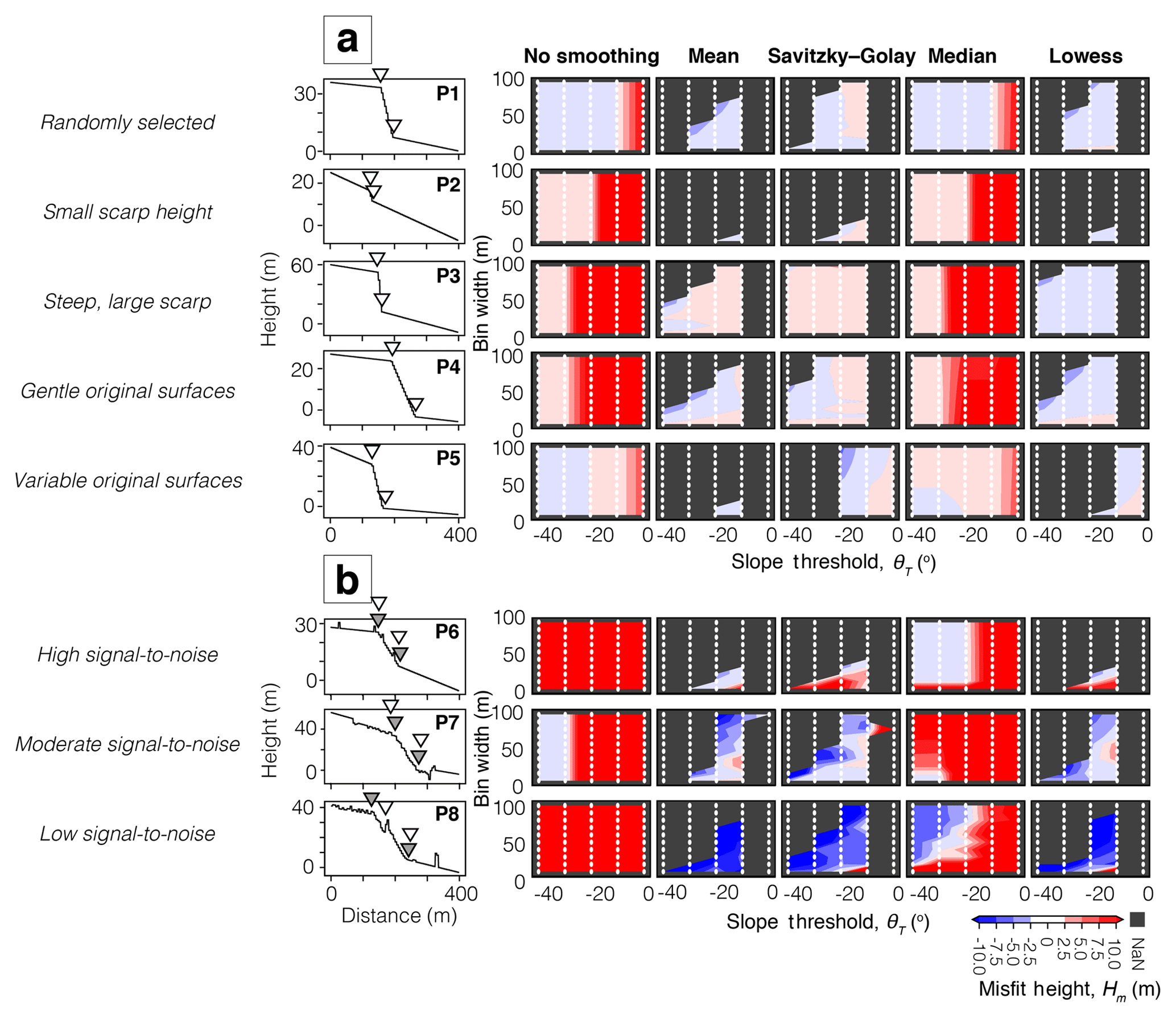
Figure 4Scarp height misfit Hm for (a) five synthetic catalogue examples with no non-tectonic features and (b) three synthetic catalogue examples with noise in the DEM caused by non-tectonic features. See the Supplement for scarp width Wm and slope misfit αm results for the catalogues with and without non-tectonic topographic features. As with Fig. 2, grey triangles show the location of the crest and base of the fault scarp based on the input parameters. White triangles denote the algorithm's best pick of the crest and base based on the misfit analysis.
3.3 Exploration of parameter space using synthetic catalogue
For each of the 1000 profiles in the synthetic catalogues, we test 250 unique combinations of algorithm parameters (filter method, bin width and slope threshold) and assess their ability to accurately determine the synthetic input parameters. Where the algorithm is not able to identify a fault scarp, a result is not recorded.
Figure 5a shows the average misfit values for the noise-free synthetic profiles where the algorithm identified a fault scarp (Eqs. 1 to 3). The best-performing bin width and slope threshold depended on the filter method used, but in general a smaller bin width and steeper slope threshold provided smaller misfit values. When not applying a filter, or using the median filter, the algorithm performed poorly; but using these filters meant the fault scarp was identified in more profiles. For the moving mean, Savitzky–Golay and Lowess filters, a gentle slope threshold (θT < 11∘) gave large misfit values, but using a steep threshold (θT ≥ 31∘) meant fault scarps were identified in less than 50 % of the profiles.
The poor algorithm performance when not using a filter, or using the moving median filter, is apparent for the average misfit values using the noisy catalogue (Fig. 5b). On average, the scarp width misfit values are larger than the scarp height misfit values. Whereas scarp height is estimated by linear extrapolation of the original surfaces and is therefore less influenced by non-tectonic topographic features and exact position of the fault scarp, scarp width is highly sensitive to the exact location of the fault scarp crest and base picked by the algorithm.
For both synthetic catalogs, the best-performing filters were the Savitzky–Golay and Lowess filters; the slope threshold with the smallest total misfit (Eq. 4) was 21∘, and a bin width of 50 m or smaller was found to perform better than a larger bin width. Thus, these are the optimal filters which we choose to employ on the real data, using bin width and slope thresholds tailored to the local environment.
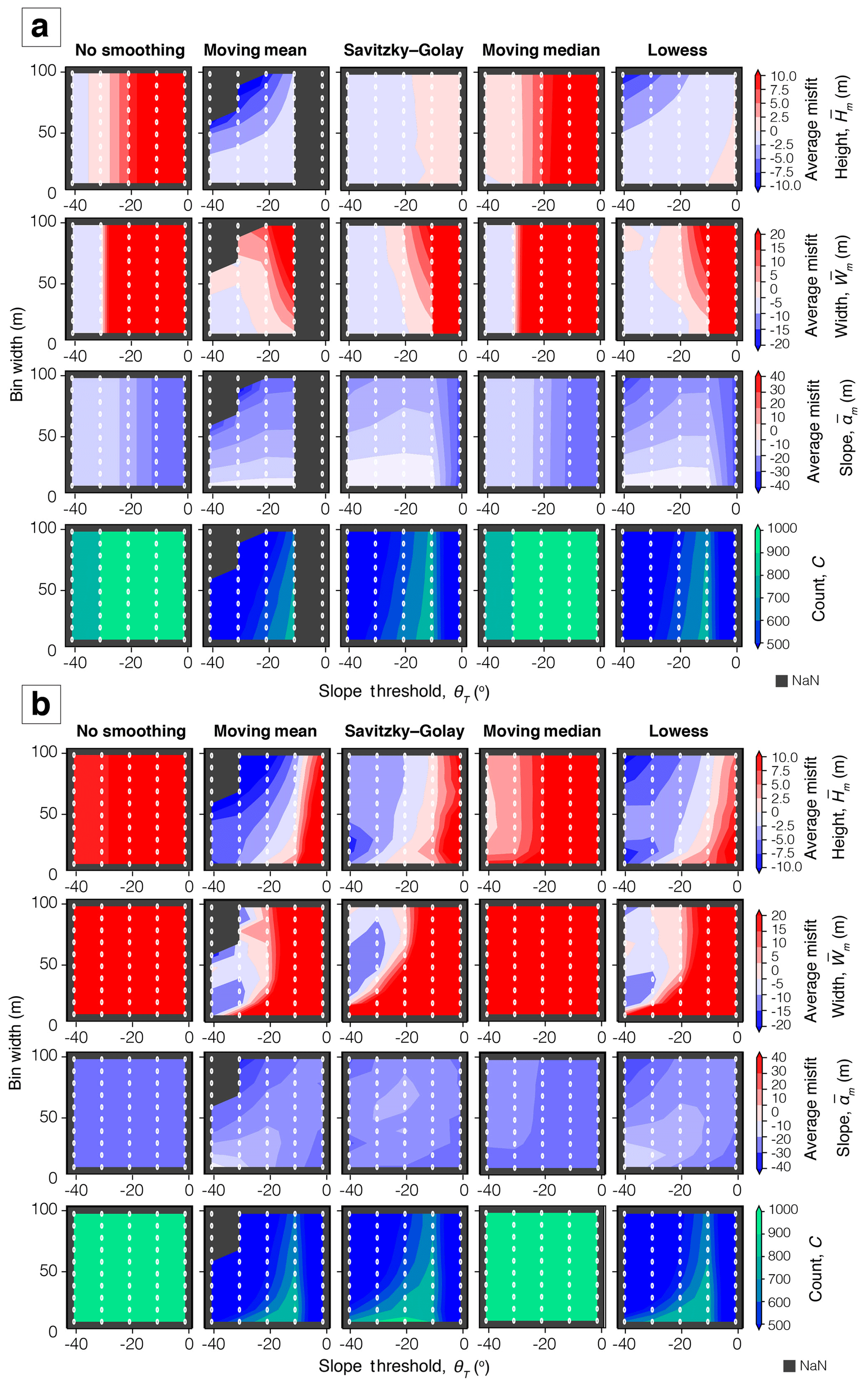
Figure 5The average misfit and count for 1000 (a) noise-free and (b) noisy synthetic catalogue fault scarps, where by “noise” we refer to non-tectonic topographic features leading to ambiguity in the DEM. Grey values denote no fault scarp was identified for all profiles. For resolutions of 5, 10 and 30 m, see the Supplement.
For the Shuttle Radar Topography Mission (SRTM), TanDEM-X and Pleiades DEMs, hillshade and slope maps were produced in QGIS 2.18 and used to identify the breaks in slope associated with the Bilila–Mtakataka fault, i.e. the scarp. Figure 6 shows the hillshade image produced by each DEM for an area of the Bilila–Mtakataka fault scarp. The scarp trace was manually picked from each hillshade image and is shown by a red line. Large-scale changes in scarp trend can be identified using the SRTM DEM (box A; Fig. 6); however, small-scale changes may not be identifiable (boxes B and C; Fig. 6).

Figure 6Bilila–Mtakataka fault scarp hillshade DEM examples using SRTM 30 m, TanDEM-X 12 m and Pleiades 5 m DEMs. The black arrows represent the fault scarp trace picked using each DEM. Box A represents the typical trend of the Bilila–Mtakataka fault scarp, boxes B and C show changes in variation in scarp trend.
We use the station lines toolbox in QGIS to draw profile lines perpendicular to the manually picked fault scarp trace. The total length of profile x was set to 400 m. To obtain accurate calculations of the scarp's morphological parameters (especially width and slope), profiles need to be taken perpendicular to the scarp trend. Therefore, where the scarp trend varies considerably, such as at the ends of fault segments and at linking structures, failing to account for the small changes in scarp trend may lead to inaccurate morphological measurements. To prevent the station lines from being drawn oblique to the true fault scarp, resulting from small-scale changes in scarp geometry, the distance between nodes (points picked on the fault scarp that when joined represent the scarp trace) should be significantly less than the distance between profiles. Here, we select scarp-perpendicular profiles at intervals of 100 m along the fault scarp trace and therefore use a nodal distance of ∼ 20 m. Therefore, as the resolution of the TanDEM-X DEM is smaller than the nodal distance, we use this to pick the surface trace of the Bilila–Mtakataka fault scarp.
A total of 913 scarp profiles were extracted from the SRTM, TanDEM-X and Pleiades 5 m DEMs, for ∼ 90 km of the Bilila–Mtakataka fault scarp that was covered by the Pleiades DEM, starting ∼ 7.4 km from the northern fault end (Fig. 1b). Due to clouds over the fault scarp on the Pleiades optical images, 26 profiles between 94 and 97 km from the northern fault end were removed. Elevation values were taken along each profile at a spacing equal to the resolution of the DEM (e.g. 5 m for the Pleiades DEM).
4.1 Algorithm results (Pleiades 5 m DEM)
To test the algorithm using a range of resolution datasets we first use the Pleiades profiles along the Bilila–Mtakataka fault. A manual analysis is conducted for 20 profiles, taken at increments of ∼ 5 km along the Bilila–Mtakataka fault scarp (Fig. 7). A misfit analysis is performed by comparing scarp parameters estimated manually and from the automated analysis.
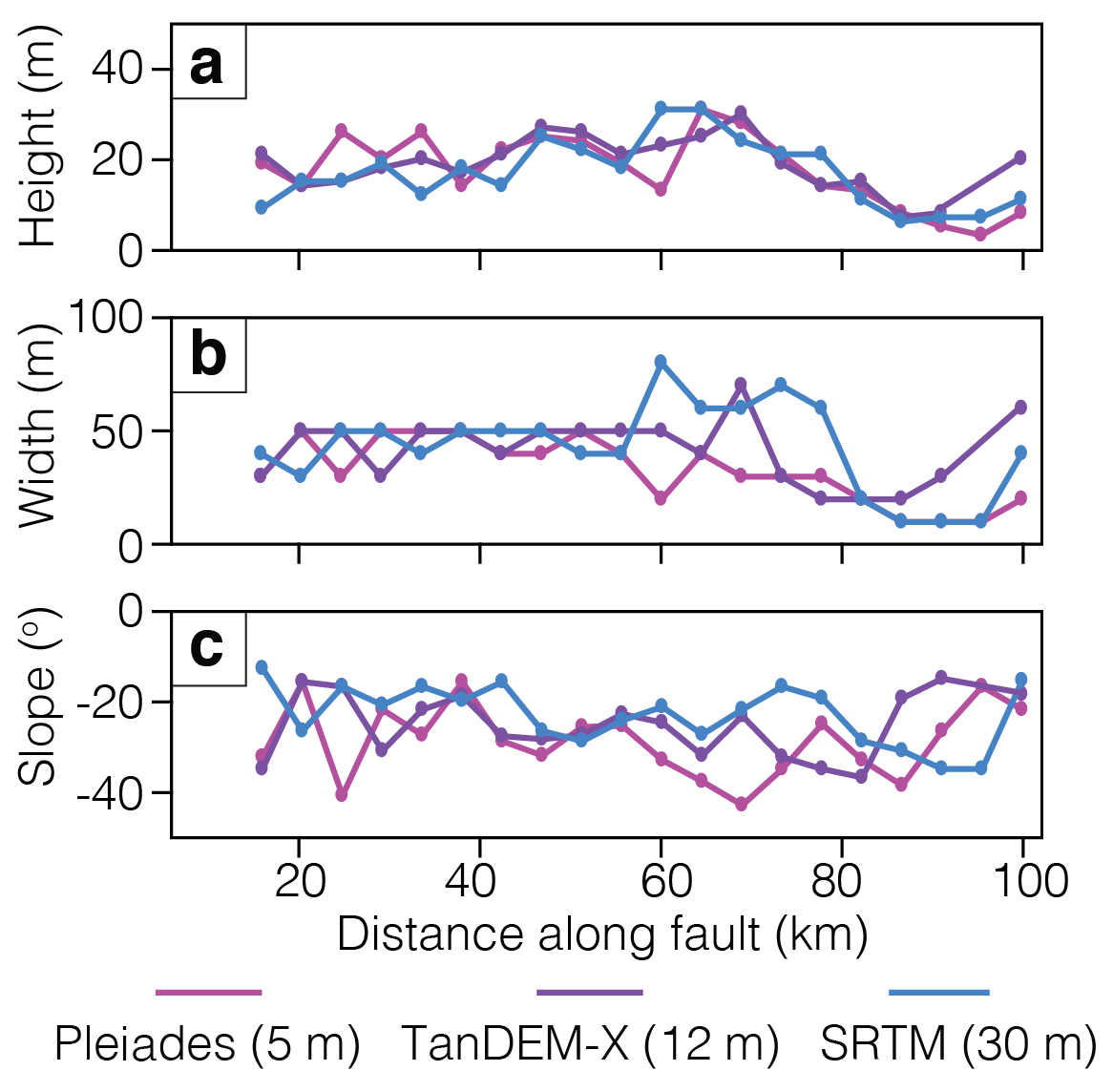
Figure 7Manual Bilila–Mtakataka fault profile for (a) height H, (b) width W and (c) slope α taken at ∼ 5 km intervals using the Pleiades 5 m, TanDEM-X 12 m and SRTM 30 m DEMs. For tabular results, see the Supplement.
Based on the algorithm performance in the synthetic tests, we only use the Savitzky–Golay and Lowess filters. The maximum bin width is reduced to 49 m, and slope threshold limits are 11 and 26∘, with increments of 5∘. We find that the algorithm using the Lowess filter, on average, had smaller misfit values and identified a greater number of fault scarps than that using the Savitzky–Golay filter (Fig. 8). As with the synthetic tests, larger bin widths and steeper slope thresholds generated smaller misfit values, especially for scarp width; however, they also identified fewer fault scarps. The algorithm using the Savitzky–Golay filter gave a large width misfit (> 20 m), except when using the largest bin widths and steepest slope thresholds in the study. Based on the total misfit value, the best results were achieved by the Lowess filter when bin width is 39 m, and a slope and slope derivative thresholds were 21 and 5∘ m−1, respectively. The average misfit values using this algorithm setup were m, m and ∘. These values are specific to this example and would vary according to DEM resolution, scarp characteristics and location.
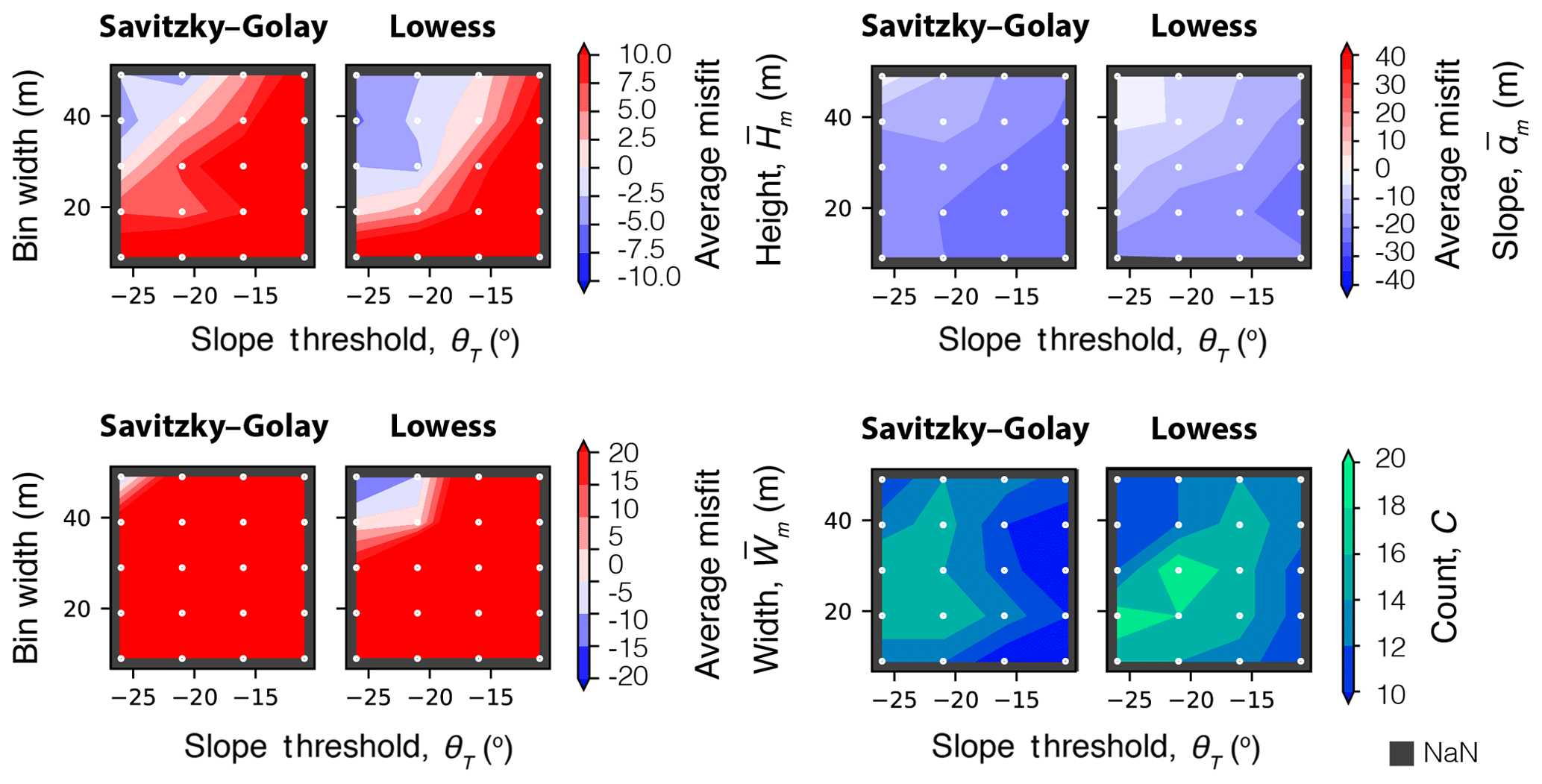
Figure 8Average misfit values between algorithm and manual scarp parameters for 20 Bilila–Mtakataka fault profiles using the Pleiades 5 m DEM.
Using the best-performing parameters, the algorithm was able to identify a fault scarp for 79 % of the 913 profiles. A histogram of the scarp height, width and slope, as well as the mean and standard deviation (σ), is shown in Fig. 9a (black). The average Bilila–Mtakataka fault scarp height, width and slope were 19 m (±17 m), 73 m (±71 m) and 20∘ (±12∘), respectively. However, as the standard deviation was of the same order of magnitude as the values themselves, this suggests there was a wide spread of results due to natural variability. Furthermore, the extremes exceeded the minimum and maximum values obtained in the manual analysis.
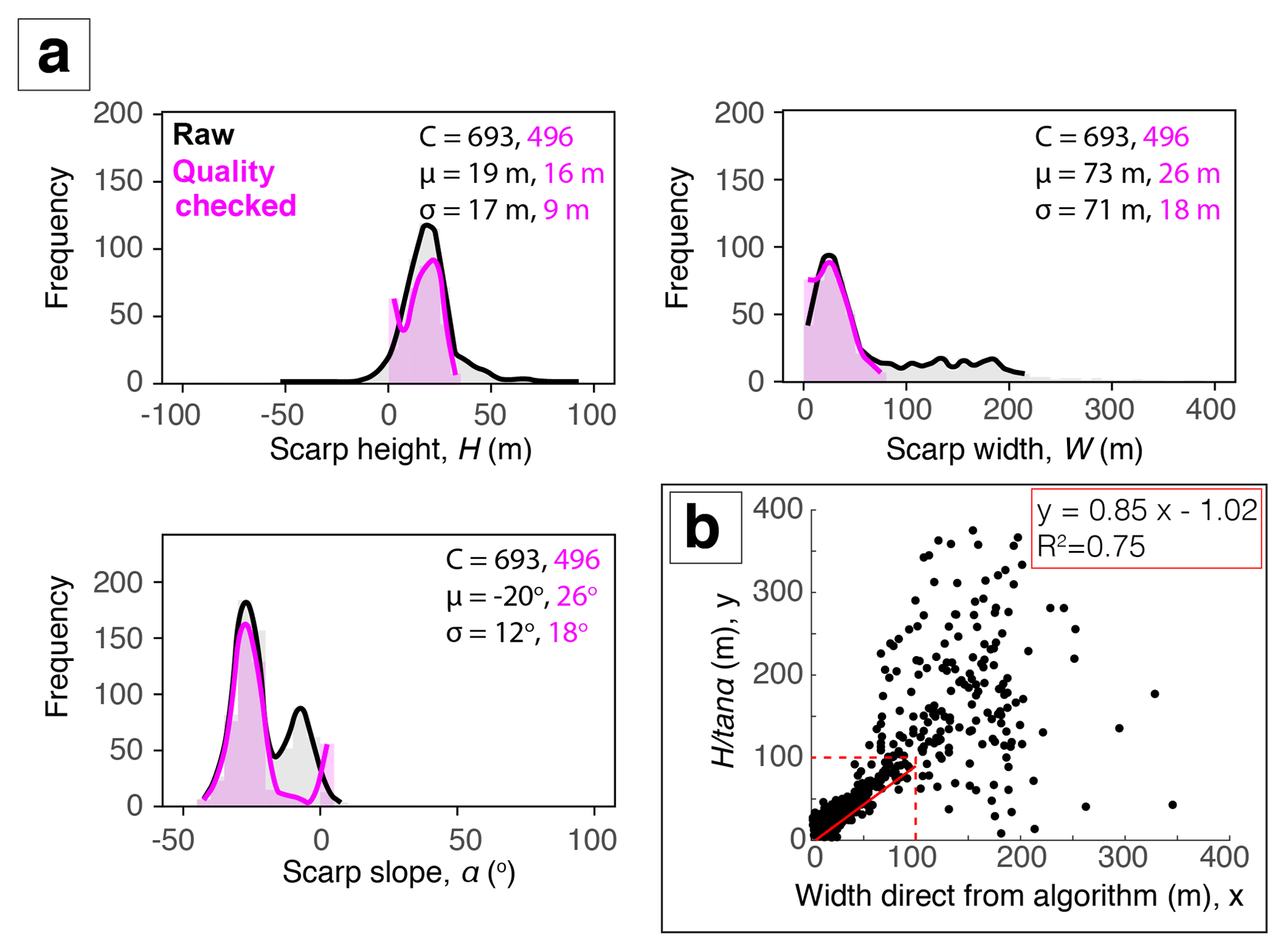
Figure 9(a) Histogram of the estimated scarp parameters for the Bilila–Mtakataka fault for all (raw) algorithm estimates (black) and post-quality-checked (pink) results. (b) A comparison between the scarp width obtained directly from the algorithm and the scarp width calculated using the algorithm's scarp height and slope values (). A linear regression is applied where width is less than 100 m.
4.1.1 Resolution analysis
Manual analyses were performed for the 20 chosen profiles along the Bilila–Mtakataka fault scarp using the TanDEM-X and SRTM DEMs, and compared to the Pleiades DEM manual results (Fig. 7). Scarp height estimates between manual analyses differed by a maximum of 18 m, width by up to 60 m and slope by up to 24∘, but the average differences were much lower: ∼ 4 m, ∼ 13 m and ∼ 8∘, respectively. The calculated scarp height and slope were the smallest and most gentle using the SRTM DEM, and tallest and steepest using the Pleiades DEM, likely due to the differing DEM resolutions.
The algorithm was then run for the 913 fault scarps using the TanDEM-X and SRTM DEMs, using the best-performing algorithm setup found for the Pleiades analysis. For plots from this resolution analysis, see the Supplement. Although the misfit values were comparable regardless of DEM resolution, the lower the resolution, the fewer fault scarps were identified: 69 % for TanDEM-X and 64 % for SRTM, compared with 79 % for Pleiades. The standard deviation of results was smaller for both TanDEM-X and SRTM results than the Pleiades DEM, leading to fewer outliers being removed after the quality-check tests were performed. Misfit values were smaller using the higher-resolution DEMs. In agreement with the manual analysis, the algorithm scarp parameters were smaller, wider and more gentle on average using the SRTM DEM, but the algorithm was still able to identify scarps with heights less than 5 m.
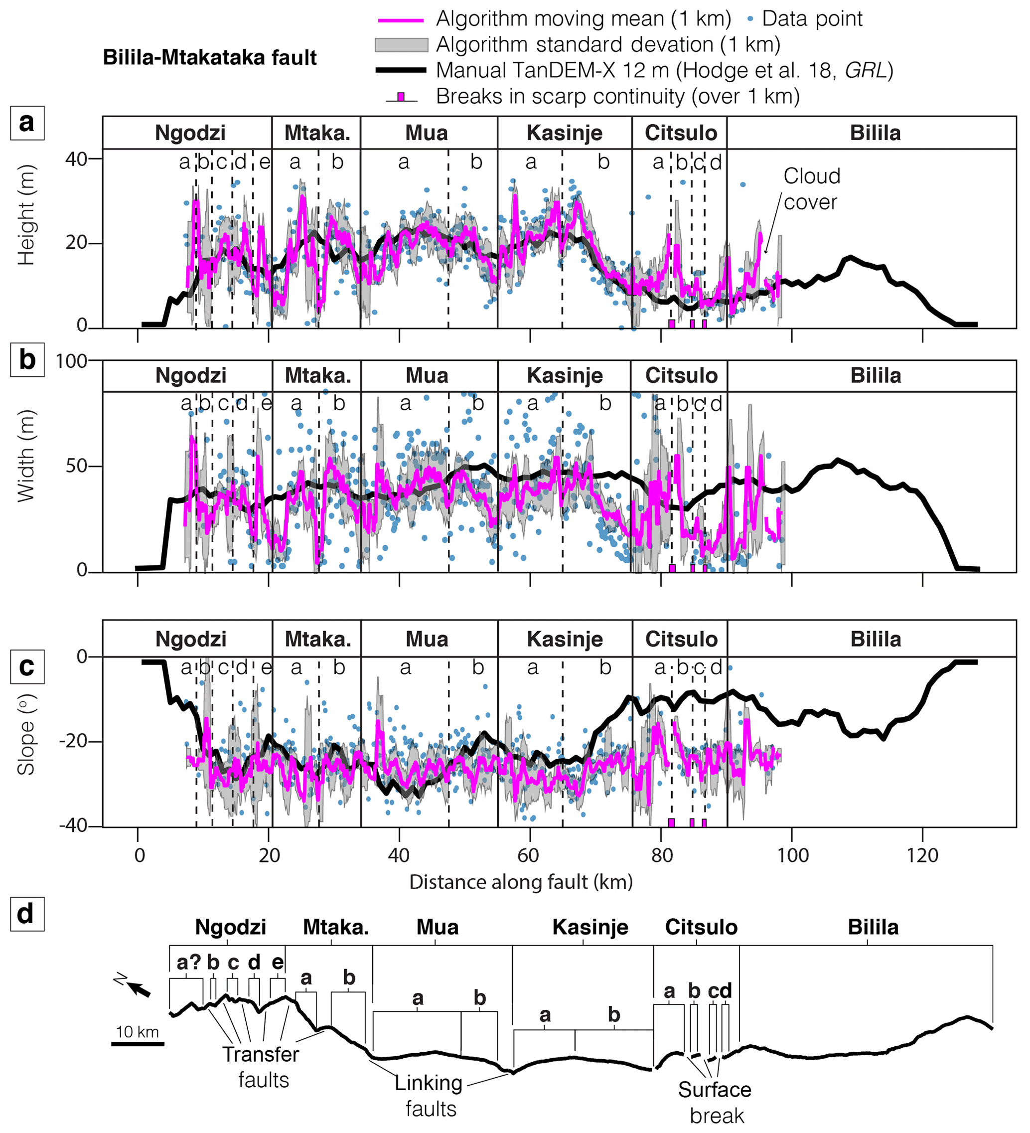
Figure 10Panels (a)–(c) show the height, width and slope profiles for the Bilila–Mtakataka fault scarp using the Pleiades DEM, indicating the major segments proposed in Hodge et al. (2018b) (Ngodzi, Mtakataka, etc.) and newly identified secondary segments (a, b, etc.) from this study. (d) A map view showing fault structural segmentation, breaks in scarp and the location of inferred linkage structures.
The average scarp height, width and slope obtained through the algorithm using each DEM were similar. The difference in scarp height between resolutions was smallest between Pleiades and TanDEM-X (2σ < 10 m) and largest between TanDEM-X and SRTM (2σ ∼ 12 m). The greatest difference in algorithm performance between resolutions was found for scarp width (40 m > 2σ > 20 m), whereas the difference between scarp slope using each resolution typically was less than 15∘. The difference in scarp height between resolutions did not show any clear along-strike pattern and was on average less than 5 m. Using a moving mean, the along-strike changes in scarp parameters between DEMs are similar and match the manual analyses well. For a scarp whose height is comparable to that of the Bilila–Mtakataka's, we find that using a low-resolution DEM (i.e. 30 m SRTM) does not profoundly affect the results; however, for smaller scarps and for accurate slope calculations, a high-resolution DEM is more appropriate.
We have shown that an automated approach performs well in comparison to a manual analysis for the Bilila–Mtakataka fault scarp. We now apply the algorithm to three further normal fault scarps: the Malombe, Thyolo and Muona fault scarps in southern Malawi (Fig. 1). The Thyolo fault (TOF) and Muona fault (MOF) are two distinct, overlapping fault scarps. As such, they may be part of the same fault system; however, a physical connection between them is not obvious in the TanDEM-X DEM. The Malombe fault (MAF) is split into three scarps: the northern (NMAF), central (CMAF) and southern (SMAF) scarps. As the algorithm performed comparatively well using TanDEM-X DEM and the Pleiades DEM for the Bilila–Mtakataka fault, we can reliably use TanDEM-X where Pleiades is not available. Therefore, for each fault, scarp parameters were calculated using the algorithm from 400 m long scarp-perpendicular profiles taken using the TanDEM-X DEM. Nodal distance for the manually picked scarp traces is again set to ∼ 20 m and scarp-perpendicular profiles are taken at intervals of 100 m. For each, we select a subsample of 25 scarp profiles for a misfit analysis against a manual method (Eqs. 1 to 4) and limit our filter methods to Savitzky–Golay and Lowess.
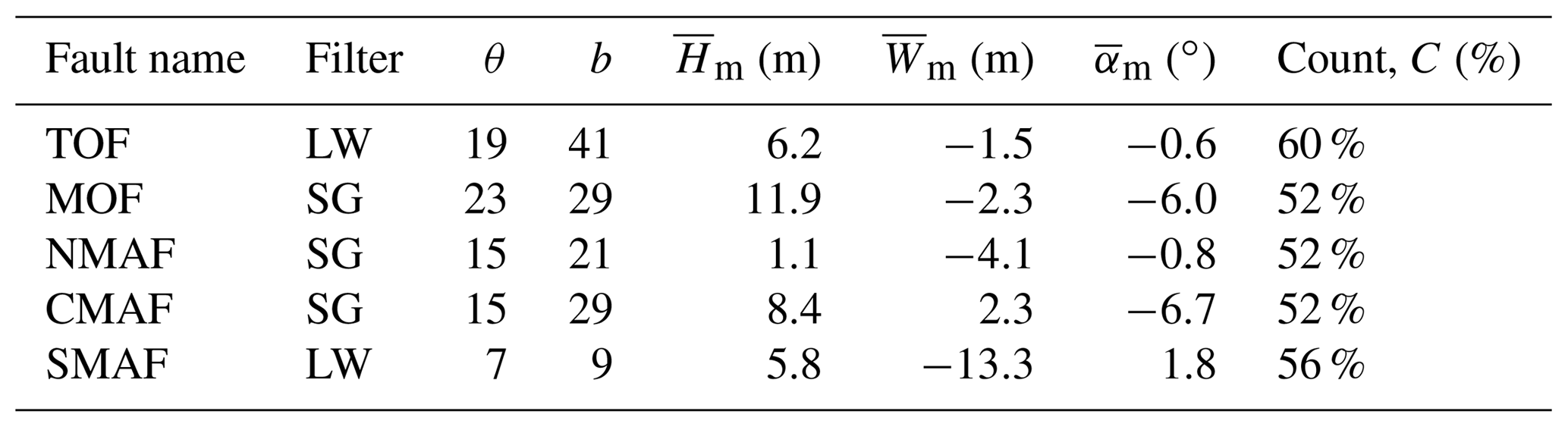
Table 2The best-performing algorithm parameters for the Thyolo, Muona and Malombe faults based on a misfit analysis using the TanDEM-X DEM: Lowess (LW) or Savitzky–Golay (SG).
5.1 Scarp morphology of Malombe, Thyolo and Muona faults (TanDEM-X 12 m DEM)
The Thyolo fault scarp is ∼ 70 km long and trends predominantly northwest–southeast (Fig. 1c). Results from the manual analysis indicate that the average height of the TOF scarp is ∼ 18 m, and its average slope is 18∘. For results, see the Supplement. The scarp of the parallel Muona fault steps to the right of the Thyolo fault and is shorter, measuring ∼ 28 km long. The faults overlap for a distance of ∼ 10 km and are separated by ∼ 5 km (Fig. 1c). The manual analysis suggests that the MOF scarp is lower (10 m on average) and more gentle (14∘ on average) than the TOF fault. The scarp width for both faults was ∼ 65 m on average, equivalent to ∼ 5 pixels. The scarp height for both faults increases by up to ∼ 9 m km−1 toward the overlap zone. Scarp measurements for the TOF within the overlap zone may contain significant errors due to the complex topography within the footwall of the Muona scarp affecting the linear regression of original surfaces. The best-performing filter for the TOF was the Lowess filter, whereas the Savitzky–Golay filter performed better for the Muona scarp (Table 2). Both faults required similar slope thresholds, but the TOF required a larger bin width (41 m compared to 29 m). The algorithm misfit values for the subsampled profiles are shown in Table 2. The algorithm performed less well for the MOF, with an average height misfit of ∼ 12 m, compared to ∼ 6 m for the Thyolo fault.
The lengths of the Malombe fault scarps are between 16 and 23 km, with the central scarp being the longest. Again, for results, see the Supplement. All of them trend approximately north–south with small local changes in scarp trend (Fig. 1d). No hard-linking structures between individual fault scarps were identifiable. Results from the manual analysis show that the scarps of NMAF and CMAF are morphologically similar, with an average height ∼ 7 m and slope ∼ 9∘. The scarp of the SMAF is smaller (∼ 4 m) and more gentle (∼ 5∘). The widths for all varied on average between 60 and 80 m. Due to their similar average slopes, the best-performing parameters for NMAF and CMAF were similar, with the Savitzky–Golay filter preferred (Table 2). The algorithm using the Lowess filter performed best for SMAF, which also performed well using smaller slope threshold and bin width than the fault scarps to the north.
The percentage of fault scarps identified for the Thyolo and Malombe profiles was between 50 % and 60 % (Table 2), yet there were a wide spread of results. To improve the algorithm outcome, first, negative scarp heights and positive scarp slopes were removed. Then, as scarp height values for both Thyolo and Malombe were normally distributed, the remaining results were quality checked using a 2σ (95 % confidence interval) threshold. Following the quality control, the percentage of scarp profiles that morphological parameters were measured for was ∼ 30 % for all scarps except the southern Malombe fault (13 %). This is likely because the small and gentle SMAF scarp may be beyond the detectable limit of profiles using the TanDEM-X DEM.
6.1 Bilila–Mtakataka
In agreement with the findings from Hodge et al. (2018a), the distribution of scarp height – a proxy for the vertical displacement (Hetzel et al., 2004; Jackson et al., 1996; Keller et al., 1998; King et al., 1988) – defines six major (first-order) structural segments along the Bilila–Mtakataka fault (Fig. 10). Scarp slope is less variable than previously considered (Hodge et al., 2018a), especially within the Citsulo segment (Fig. 10c). This is likely due to the lower spatial resolution of measurements used in previous studies, where poor quality measurements – unrepeatable and inaccurate due to the reasons given in Sect. 2.1 – greatly influenced the along-strike profile. The ability to measure scarp parameters at a high spatial resolution is a major benefit of an automated algorithm. Using the traditional, manual approach, increasing the number of fault scarp profiles would dramatically increase the time required.
In addition, by increasing the spatial resolution of measurements, along-strike changes in displacement may be identified at a smaller scale. As regular, frequent spacing cannot account for scarp height differences caused by local geomorphology (i.e. erosion, deposition, non-fault related landforms), many of the measurements and signals may not be entirely tectonic (Zielke et al., 2015). A moving mean is therefore used to minimise such local influences. In Fig. 10, the moving mean window size is set to 1 km for the Pleiades algorithm results. The general trend of the algorithm results still follows the manually derived trend taken using a larger window size, but variations in height occur along strike at an even smaller scale than previously considered, as detailed below.
Changes in scarp height with a magnitude larger than the typical algorithm error (≥ 5 m) are considered to be real along-fault changes in scarp morphology. As the algorithm assumes only a single scarp surface, multi-scarps (also known as multiple scarps) or composite scarps associated with individual ruptures (Crone and Haller, 1991; Ganas et al., 2005; Nash, 1984; Wallace, 1977; Zhang et al., 1991) will be treated as a single scarp. In other words, the calculated scarp height is the cumulative vertical displacement at the surface. The results indicate that (second-order) secondary structural segments exist along the Bilila–Mtakataka fault, as typically expected for a large, structurally segmented fault (Dawers and Anders, 1995; Manighetti et al., 2015; Peacock and Sanderson, 1991, 1994; Trudgill and Cartwright, 1994; Walsh and Watterson, 1990, 1991). Faults forming hard links between major segments, and those linking secondary segments, are also observed and we discuss specific examples below.
For the Ngodzi segment, at least five small (2 to 5 km long) secondary segments, joined by high-angled linkage structures, are identifiable by the local highs and lows in scarp height (Fig. 11a). The separation-to-length ratio between each secondary segment is around ∼ 1, an ideal geometry for a transfer fault to establish (Bellahsen et al., 2013; Hodge et al., 2018b). The scarp appears to splay at the intersection between the southern-most Ngodzi secondary segment and the Mtakataka segment, potentially comprising a single, or series of, small transfer faults (Fig. 11a). A small rural settlement exists on top of the elevated surface caused by the footwalls of the two major segments; this has led to a significant amount of erosion to the scarp face, making it difficult to identify a hard link between the major segments (Fig. 11b).
The intersection between two parallel, slightly offset secondary segments on the Mtakataka segment is distinguishable by a low in scarp height. The sharp change in scarp trend at this intersection suggests the existence of a high-angled transfer fault. The Mtakataka and Mua segments are then linked by a ∼ 2 km long linking fault angled on average ∼ 35∘ from the scarp trend. The geometry between segments is most favourable for a fault bend (Hodge et al., 2018b; Jackson and Rotevatn, 2013). Furthermore, there is no evidence of a breached relay ramp.
The height of the fault scarp along the Mua segment is indicative of a single, major structural segment (i.e. bell-shaped height/displacement-length profile with slip maximum at the centre); however, a small decrease in height at ∼ 47 km may be evidence of a inter-segment zone between secondary structural segments (Fig. 11c). If so, the subtle change in scarp morphology suggests that the secondary segments initiated as separate faults but have since hard-linked and matured, as the displacement deficit is minor. At the southern tip of the Mua segment, there is a decrease in height (∼ 10 m) and change in geometry several kilometres from the northern tip of the Golomoti segment, which is marked by the Livelezi River (Fig. 11c). The river itself marks the only break in scarp continuity between the Mua and Kasinje segments. The > 45∘ change in scarp trend and slight overlap between segments suggest that the offset may have been bridged with a relay ramp that has since breached, forming a hard link, and subsequently been exploited by the Livelezi River. Similar to the Mua segment, the displacement distribution along the Kasinje segment is characteristic of a single, major segment, but a local decrease in scarp height (< 5 m) at ∼ 63 km suggests that two secondary segments may have once existed as isolated structures (Fig. 11c). These segments have since hard-linked and matured, and the cumulative displacement has reduced much of the deficit within the inter-segment zone.
Previous work has suggested that the Citsulo segment had a general zone of scarp discontinuity stretching ∼ 10 km in length (Hodge et al., 2018a). Here, we find evidence of several small breaks along the fault scarp within the Citsulo segment (Fig. 11d). Breaks are up to 2 km in length, suggesting that the Citsulo segment comprises several small (∼ 2 km), en echelon secondary segments.
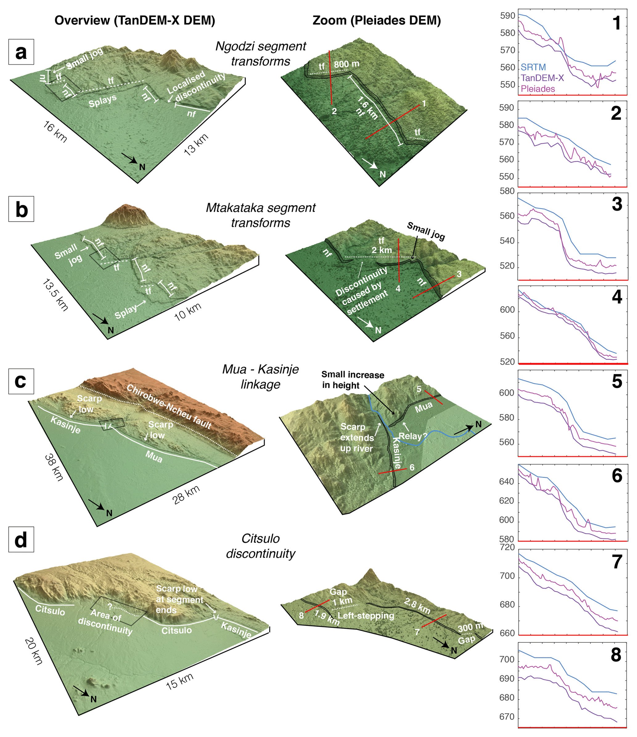
Figure 11Oblique perspective images taken from the TanDEM-X and Pleiades DEMs for the Bilila–Mtakataka fault. (a) Ngodzi segment normal (nf) and transfer faults (tf) trend in a zig-zag pattern. (b) Mtakataka segment normal and transfer faults. (c) Mua and Kasinje segments intersecting at the Livelezi River. A small increase in scarp height on the Mua segment may relate to a relay ramp linkage. (d) The Citsulo segment and area of discontinuity. Small, north-striking, left-stepping faults are offset by up to 1 km. Example profiles for SRTM, TanDEM-X and Pleiades DEMs are also shown.
6.1.1 Thyolo and Muona
Figure 12 shows the along-strike profile for the Thyolo and Muona faults. Scarp slope for both Thyolo and Muona faults is fairly uniform, averaging around ∼ 22∘ with a small standard deviation < 5∘ (Fig. 12c). Scarp height and width, however, show more variation along strike (Fig. 12a, b). We interpret three major segments along the TOF from the numerous peaks and troughs in scarp height, called TOFS1, TOFS2 and TOFS3, whose lengths are between 15 and 30 km. In contrast, the height of the shorter MOF is fairly consistent before it tapers off toward the southeastern fault end. We therefore interpret the Muona fault to consist of a single major segment. Below, we describe each major segment and any associated secondary segments and linkage structures. The faults do not appear hard-linked, likely due to the large separation-to-length ratio (⪆ 0.1), which may favour continued along-strike growth or a transfer-style link (Bellahsen et al., 2013; Hodge et al., 2018b). Below, we describe each major segment of the faults and any associated secondary segments and linkage structures.
For both TOFS1 and TOFS2, the distribution of scarp height is bell-shaped with slightly asymmetry of the TOFS2 profile toward the inter-segment zone. For TOFS1, scarp height is larger and increases from ∼ 10 m at the segment ends to ∼ 30 m at the centre; an increase in width is also observed at the centre, resulting from the consistent scarp slope. The maximum height of the TOFS2 scarp is ∼ 20 m. For both, the peaks in scarp height coincide with the apex of the convex geometry of the fault scarp (Fig. 12d). The scarp height and width of TOFS3 increase gradually toward the southeast, where the segment extends into the footwall of the MOF. The scarp height of TOFS3 within the overlapping zone between the Thyolo and Muona faults exceeds the MOF scarp height by, on average, ∼ 5 m. The standard deviation of measurements here is larger than elsewhere along both fault scarps, indicating intense local variability in scarp parameters.
The low count of scarps recognised by the algorithm along the Thyolo fault meant that we cannot conclusively interpret the existence of secondary segments. There are several > 1 km long breaks in where the algorithm could recognise a scarp along TOFS1 and TOFS2; however, the distribution of scarp heights does not conclusively imply second-order segmentation. For TOFS3, several major breaks in scarp continuity coincide with sharp changes in scarp trend. Based on these changes in trend, we interpret three secondary segments, called TOFS3a, TOFS3b and TOFS3c, and associated linkage structures (Fig. 14d). Each of these secondary segments has a length ∼ 10 km, and TOFS3c coincides with the length of the overlapping zone between Thyolo faults. There is no conclusive evidence of secondary segments along the Muona fault. Two major ∼ 4 km breaks in scarp continuity toward the segment end suggest a shorter fault scarp (∼ 20 km) than our manual analysis suggested. Large gaps between profiles, typical of a manual analysis, may therefore fail to account for small-scale changes in morphology and over/underestimate fault lengths.
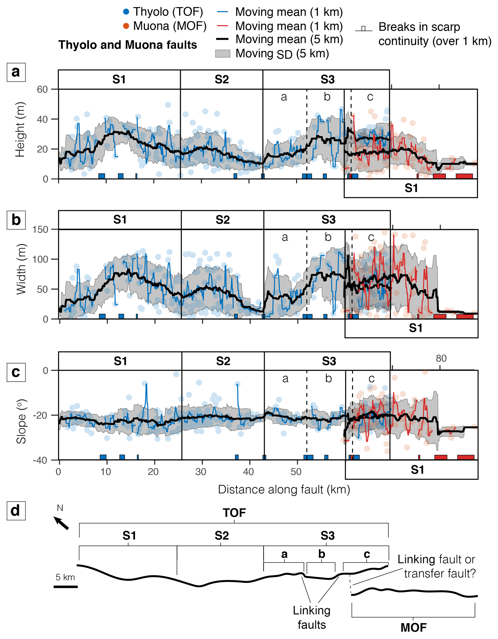
Figure 12Panels (a)–(c) show the height, width and slope profiles for the Thyolo and Muona fault scarps using the TanDEM-X DEM. (d) A map view showing fault structural segmentation, breaks in scarp and the location of inferred linkage structures.
6.1.2 Malombe
In agreement with the manual analysis, the slopes of the NMAF and CMAF fault scarps are remarkably similar, averaging ∼ 18∘ (Fig. 13). Based on the remarkably uniform scarp height, averaging ∼ 8 m, the NMAF appears to comprise a single major segment. A small break in scarp continuity and ∼ 10 m decrease in scarp height along the CMAF at ∼ 24 km suggest an inter-segment zone between two major segments, called CMAFS1 and CMAFS2 (Fig. 14b). The scarp height of CMAFS1 is the largest of all Malombe faults, averaging ∼ 8 m. The distribution of scarp height along the CMAFS1 is roughly bell-shaped with an asymmetry leaning toward the NMAF. The height of the short CMAFS2 segment decreases by around 1 m km−1 from north to south. A major ∼ 6 km break in the SMAF scarp continuity implies either two major segments, SMAFS1 and SMAFS2, or a continuous deeper fault that has not broken the surface continuously. The scarp height for the SMAF is relatively constant, averaging ∼ 5 m, and does not display a bell-shaped profile. No secondary segments were inferred from the distribution of scarp height along any Malombe fault scarp. The longest segment, CMAFS1 (18 km), does comprise several breaks in scarp continuity and changes in morphology typical of second-order segmentation; however, a higher spatial resolution of measurements would need to confirm this.
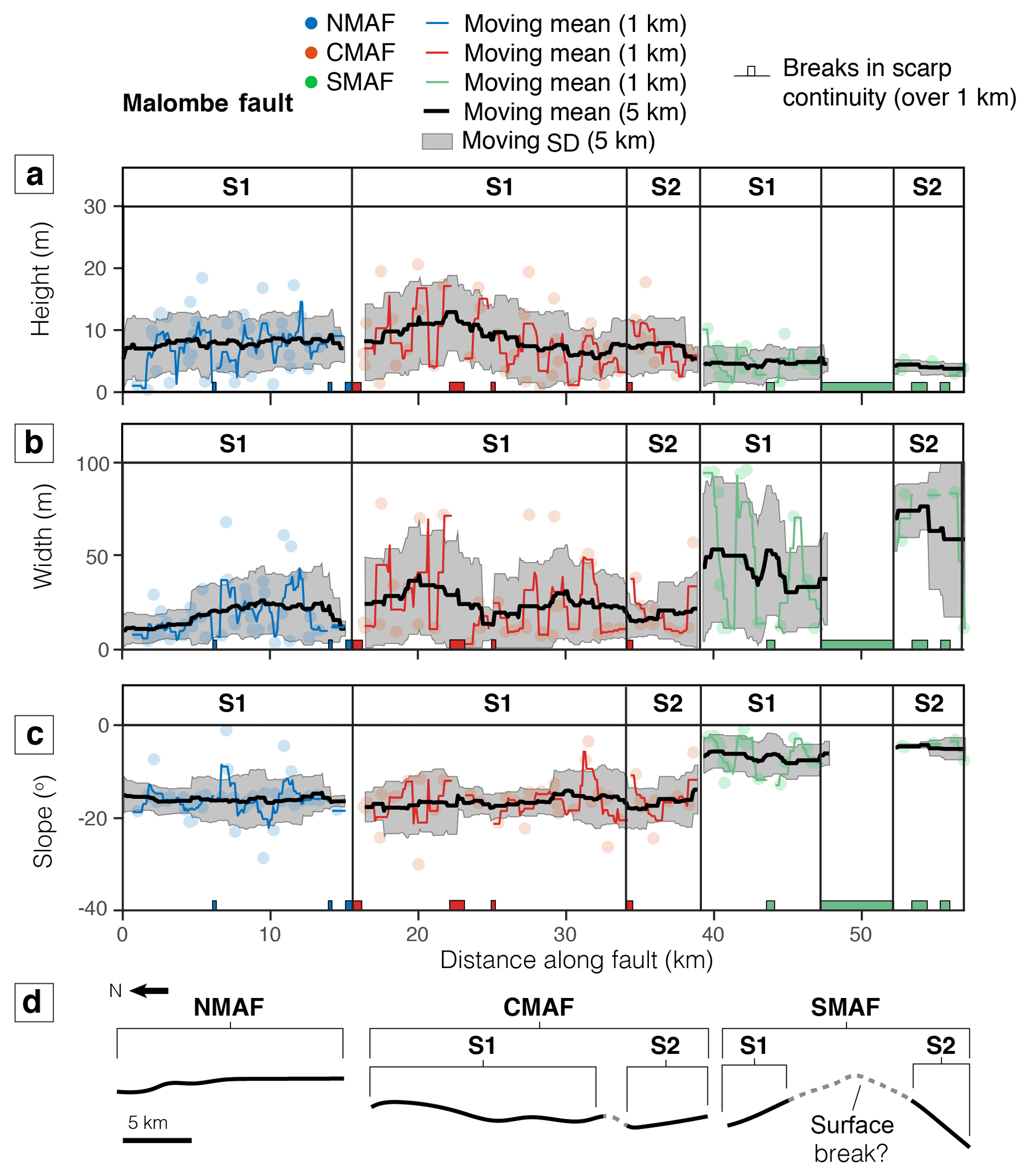
Figure 13Panels (a)–(c) show the height, width and slope profiles for the Malombe fault scarps using the TanDEM-X DEM. (d) A map view showing fault structural segmentation, breaks in scarp and the location of inferred linkage structures.
7.1 Algorithm performance
In this study, we developed an algorithm for calculating the height, width and slope of a fault scarp from scarp elevation profiles: Scarp PARameTer Algorithm (SPARTA). A series of sensitivity analyses were performed using a synthetic catalogue prior to using the algorithm on real fault scarps. The benefits of creating a synthetic catalogue are two-fold: (1) a vast number of scarp profiles can be built to improve the performance of the algorithm through an in-depth misfit analysis, and (2) by creating a synthetic catalogue that mimics the typical fault scarp morphology of interest and performing a sensitivity test for resolution, the benefits of high-resolution satellite data can be assessed prior to purchasing costly data (see the Supplement for synthetic catalogue test results). The synthetic catalogue should mimic the typical fault scarp morphology of interest. This can be achieved by selecting a prior catalogue parameters based on initial findings using a free, low-resolution data DEM (e.g. SRTM). The general morphology of the fault scarp and climatic conditions heavily influence the chosen catalogue parameters. For example, for regions where transport-limited fault scarps and vegetation are typical, the catalogue parameters can include diffusion and non-tectonic topographic features. In contrast, for regions typical of diffusion-limited fault scarps and limited vegetation, no diffusion and fewer/smaller non-tectonic features can be used.
We found that the major influence on algorithm performance was the amount of non-tectonic features within the elevation profiles. Profiles that are ambiguous because of non-tectonic topographic features will likely require the inclusion of a filter within the algorithm. In contrast, the algorithm may perform well without a filter for profiles where the scarp is clear of other topographic irregularities. In general, the algorithm was able to calculate scarp height and slope with a smaller misfit, compared to a manual analysis, than scarp width. The performance was improved by calculating scarp width based on the estimated scarp height and slope, rather than directly (Fig. 9b). However, this approach assumes scarp planarity and therefore precludes use of the results for scarp degradation analysis or interpretation of single-rupture versus composite scarps.
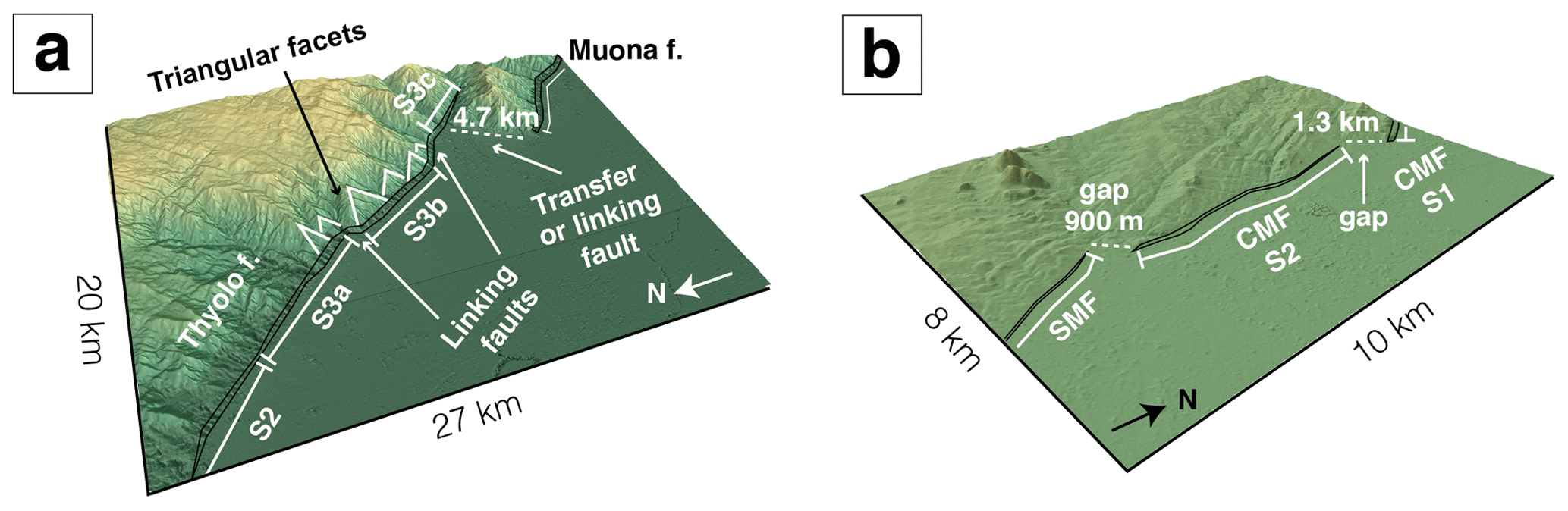
Figure 14Oblique perspective images taken from the TanDEM-X DEM for sections of the (a) Thyolo and Muona faults and (b) Malombe fault scarps. (a) The secondary segments along TOFS3 of the Thyolo fault, showing the triangular facets synonymous with an mature scarp and the structure that connects the Thyolo and Muona faults. (b) The soft linkage between the central fault segments (CMAFS1 and CMAFS2) and between the central and southern faults; each are offset by around 1 km.
In our case studies, the percentage of fault scarps where the algorithm was able to identify the scarp varied between ∼ 50 % and ∼ 80 %. Lower returns coincided with fault scarps identified manually to contain large breaks in scarp continuity. Although the algorithm selects the best-performing parameters from the misfit analysis, individual profiles may still fit poorly. Quality checks were applied to remove outliers and improve the results, but this decreased the number of identified scarps for each case study to between ∼ 15 % and ∼ 55 % of profiles. It is possible that the selection of scarps biases the analysis of scarp height. However, any bias would be towards the larger, sharper scarps and the effect is likely to be minor in comparison to the effects of erosion which tend to reduce estimates of scarp height.
The performance of the algorithm was not significantly affected by DEM resolution, but a number of differences were apparent between datasets (see the Supplement for a more detailed discussion). The lower the DEM resolution, the smaller the number of identifiable fault scarps, but the smaller the standard deviation of parameters. We found that a 30 m resolution DEM identified on average 20 % fewer fault scarps than a high-resolution 5 m DEM. Scarp width and slope calculated by the algorithm were on average wider and more gentle using a low-resolution DEM. In general, though, we found that for these southern Malawi faults, the use of expensive, high-resolution DEMs in quantifying large-scale changes in scarp height over the scale of an entire fault, did not bring any additional benefits over using a medium- or low-resolution DEM. An exception is where scarp height is smaller than the elevation changes produced by topographic noise such as vegetation. This is an important finding if using this algorithm to study fresh ruptures, which are apparent as steep faces of fault scarps (Wallace, 1977), or scarps whose vertical displacement is less than 10 m, for which we recommend using a very high-resolution (≤ 1 m) DEM and a large slope θ threshold.
Although our algorithm performed well against a number of manual analyses, the algorithm has some limitations including the reliance on manually picking the fault scarp trace. As low-resolution DEMs smooth small-scale changes in scarp trend, this is most pertinent when using a high-resolution DEM and a high spatial frequency of sample points (Fig. 6). In addition, here, we have used scarp-perpendicular scarp profiles, which may not be appropriate for oblique slip faults or sections of the scarp that trend at a high angle to the slip vector (Mackenzie and Elliott, 2017). Slip vectors could not be measured for the southern Malawi faults (Hodge et al., 2018a). Using the regional extension direction, the total surface slip may not be truly represented by the scarp height for the northern BMF segments, nor the Thyolo and Muona faults. If the slip vector of a fault is known, this can be accounted for in the algorithm.
We found that the distance between nodes (vertices of the scarp trace) should not exceed an order of magnitude above the horizontal resolution of the DEM. However, as long as the large-scale fault trend is correctly chosen, a wide profile length x (here set to around 4 times the largest scarp width) should cover a sufficient amount of the upper and lower original surfaces for the algorithm to calculate the scarp height correctly. In addition, as the algorithm uses a fixed slope threshold, if there are a lot of non-tectonic features within the data, or there is a significant amount of heterogeneity in the scarp's morphology, along-strike, small or gently dipping fault scarps may not be identified by the algorithm. This can be alleviated by either (1) identifying morphologically different parts of a fault scarp and running the algorithm on these profiles separately, as we have done for Malombe, or (2) following the first algorithm run, running the algorithm again on poorly resolved regions, including a manual analysis to identify the best algorithm parameters to use. We suggest that the algorithm may face additional limitations in a more complex or varying terrain than considered here.
7.2 Normal faults in southern Malawi
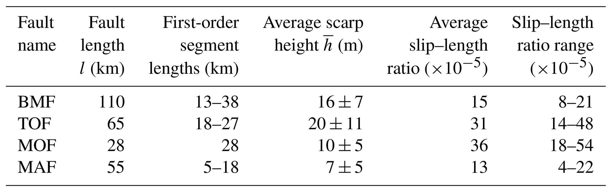
As fault scarps are indicative of past earthquake events (Wallace, 1977), we use our geomorphological findings to better understand the rupture history for each fault. As outlined in the introduction, interpreting this history is complicated by not knowing whether the scarp formed in one or more events. Making the end-member assumption that the scarp is formed from a single earthquake event, the average scarp height can be used as a proxy for average coseismic slip (Morewood and Roberts, 2001) to calculate the slip–length ratio (Scholz, 2002). The typical global slip–length ratio range for a single earthquake is 10−5 to 10−4 (Scholz, 2002). Note, however, that fault slip at the surface may be several times less than the slip at depth (Villamor and Berryman, 2001). We simplify the length value to be the straight-line distance between the tips of the surface trace, which is less than the length of the irregular surface trace. Here, we found that the ∼ 65 km long Thyolo and ∼ 110 km long Bilila–Mtakataka faults have scarp heights that average ∼ 20 ± 11 m and ∼ 17 ± 7 m, respectively. The average scarp height of the Bilila–Mtakataka fault found here is larger than found previously (Hodge et al., 2018a; Jackson and Blenkinsop, 1997), but this is because only ∼ 90 km of the fault was analysed and the non-analysed sections of the Bilila–Mtakataka fault, predominantly the ∼ 35 km long Bilila segment, have a smaller scarp height. Due to the close agreement between algorithm and manual calculations, we hereafter combine the average scarp height from (Hodge et al., 2018a) for the area that was not analysed in this study (0–8 km, 7 ± 3 m and 98–110 km, 10 ± 6 m), with the findings from this study. This gives a weighted average scarp height of ∼ 16 ± 7 m. The average scarp heights of the ∼ 28 km long Muona fault and the ∼ 55 km long Malombe fault are ∼ 10 ± 5 m and ∼ 7 ± 5 m, respectively. If each scarp is representative of a single earthquake event, then the average slip–length ratios for each fault (1–4 × 10⁻⁴) fall on or above the upper limit of the typical global range (Scholz, 2002). To account for errors in fault length measurements, we apply an uncertainty of 1 %.
Table 3Slip–length ratios for southern Malawi faults: Bilila–Mtakataka (BMF), Thyolo (TOF), Muona (MOF) and Malombe (MAF).
Whilst large slip–length ratio values are rare (Middleton et al., 2016), they have been calculated for the 1897 ∼ Mw 8.1 Assam earthquake (Bilham and England, 2001), the 2001 ∼ Mw 7.6 Bhuj earthquake (Copley et al., 2011) and the Mw 7.6 1999 Chi-Chi earthquake (Lee et al., 2003). The slip–length ratios for the normal-faulting 2008 Yutian and 2006 Mozambique earthquakes were 1–2 × 10⁻⁴ although both were blind earthquakes which did not rupture the surface (Copley et al., 2012; Elliot et al., 2010). The only well-documented surface-rupturing event with a recorded slip–length ratio within the EARS was for the ∼ Ms 6.8 1928 Kenya earthquake (Ambraseys and Adams, 1991), whose 1 m scarp could be traced for ∼ 38 km at the surface (Ambraseys, 1991b), resulting in a ratio of ∼ 2.8 × 10⁻⁵.
Abnormally large slip–length ratios may be a result of overestimating surface slip, as shown by Middleton et al. (2016) for the ∼ Mw 7.3 1739 Yinchuan earthquake in China, whose original slip–length estimate was 1.3 × 10⁻⁴. They recalculated this value to be 3.8 × 10⁻⁵ based on a slightly shorter surface rupture length (87 km compared to 88 km) and a smaller average slip value (3.3 m compared to ∼ 12 m). Thus, the new slip–length ratio is within the global range (Scholz, 2002). Here, even when accounting for measurement errors within the satellite data and algorithm calculations, we find that each of our southern Malawi fault scarps have slip–length ratios larger than the global mean (Scholz, 2002).
7.2.1 Number of events
The slip–length ratio calculation above makes the assumption that the current scarp was formed by a single earthquake event. Therefore, the large values for our southern Malawi faults either are a result of local effects, such as large seismogenic thickness (Jackson and Blenkinsop, 1993), or suggest that each scarp has been produced by multiple earthquake events. Whether the current scarps were each formed by single, large slip rupture or multiple, smaller slip ruptures is an important question for assessing the seismic hazard in the region. As the surface length is well constrained and is in fact smaller than the longest faults in the EARS (Morley, 1999; Vittori et al., 1997), the validity of the slip–length ratios are governed by the scarp height for each fault (Table 3).
Well-documented, historically recorded continental normal fault scarps formed by single earthquake events typically have a height less than 10 m (Walker et al., 2015; Zhang et al., 1986). A short, incomplete earthquake catalogue (Midzi et al., 1999) and slow extension rates along the Malawi Rift (Saria et al., 2014; Stamps et al., 2008) leading to long recurrence intervals (Hodge et al., 2015) mean that there is a lack of recorded earthquake events in the Malawi Rift with visible surface offsets. Historical earthquakes that have occurred in the Malawi Rift, either did not rupture the surface, such as the 1989 ∼ Mw 6.1 Salima earthquake (Jackson and Blenkinsop, 1993), or had small (< 1 m) amounts of surface displacement, such as the 2009 Ms 6.2 Karonga sequence (Biggs et al., 2010; Macheyeki et al., 2015). The latter resulted in an average scarp height of ∼ 10 cm and surface rupture length of 9 km. There are a number of reported events within the EARS, but outside the Malawi Rift, that have been suggested to have produced significant (> 10 m) vertical displacement. For example, within the Rukwa Rift just north of the Malawi Rift, there is evidence of a Late Pleistocene earthquake producing ∼ 10 m of uplift in the Songwe Valley, Rukwa (Hilbert-Wolf and Roberts, 2015). Constraining this displacement to a single event, however, is challenging due to its age. This event occurred within the same region reported to have hosted one of the largest recorded earthquakes on the EARS, the 1910 ∼ M 7.4 Rukwa earthquake (Ambraseys, 1991a). The most likely fault to have hosted this event is the Kanda fault, which has a reported maximum scarp height of 50 m (Vittori et al., 1997). The Kanda scarp is reported to comprise a fresh face synonymous with a recent rupture (Vittori et al., 1997); but due to the a lack of absolute age estimates on the Kanda fault scarp, and because the region has experienced frequent earthquakes since the Late Pleistocene (Hilbert-Wolf and Roberts, 2015), its unclear whether this scarp was formed by a single event. More modest scarp heights such as the 1.5 m scarp along the ∼ 50 km Katavi fault have been recorded in the Rukwa Rift (Kervyn et al., 2006). The Katavi fault, however, is considered to be a possible aftershock site resulting from the 1910 event (Kervyn et al., 2006) and does not reflect a main earthquake event.
Using the global mean slip–length ratio of 5 × 10⁻⁵ (Scholz, 2002), and assuming slip on each fault is pure normal, the number of events required to generate the current scarp heights along the Bilila–Mtakataka, Thyolo, Muona and Malombe faults is between 2 and 5, with the Thyolo fault requiring the greatest number of events. This does not account for vertical erosion between events and therefore may be an underestimate.
7.2.2 Displacement profile and segmentation
Fault scarps developed through multiple events have been observed in many regions (Crone and Haller, 1991; Ganas et al., 2005; Nash, 1984; Wallace, 1977; Zhang et al., 1991). Multiple earthquake events have also been suggested as a method for fault development, where large faults form iteratively through fault growth and linkage of smaller fault segments (Anders and Schlische, 1994; Cowie and Scholz, 1992; Peacock and Sanderson, 1991). Single earthquake ruptures can have significant along-strike variability in on- and off-fault deformation and in slip propagated to the surface (Hamling et al., 2017; Milliner et al., 2016; Wang et al., 2014). Therefore, although we interpret the scarps as likely produced by several earthquakes, we cannot exclude the possibility that variations in scarp morphology also reflect variability in surface fault slip within a single earthquake.
The along-strike pattern of scarp height for the Bilila–Mtakataka (at least up to the Citsulo segment) and Malombe fault scarps show a symmetrical bell-shaped profile, with the maximum scarp height near the centre of the fault (Manighetti et al., 2001; Nicol et al., 2010; Peacock and Sanderson, 1991; Walsh and Watterson, 1987, 1990), whereas the Thyolo fault displays a distinctive asymmetric, triangular displacement-length profile (Manighetti et al., 2001, 2009, 2015; Nicol et al., 2005; Soliva and Benedicto, 2004). Height along the Thyolo fault scarp decreases southeastward before increasing toward the overlap zone with the Muona fault. Geological maps indicate that there may be a physical connection between the Thyolo and Muona faults (Habgood et al., 1973). The triangular distribution and tapering of scarp height along the Thyolo fault scarp may denote that the direction of long-term fault propagation is southeastward onto the Muona fault (Manighetti et al., 2001, 2015).
By observing the along-strike variation in scarp height for each fault, we found evidence for structural segmentation on each fault. We found that the ∼ 110 km long Bilila–Mtakataka fault comprises six major segments, the ∼ 70 km long Thyolo fault has three, and the ∼ 25 km long central Malombe fault has two. The Muona fault did not show signs of along-strike segmentation and is considered a single major segment. Segments along the Thyolo fault and Bilila–Mtakataka fault, with the exception of fault splays within the Citsulo segment, have hard-linked. These hard links imply fault maturity (Trudgill and Cartwright, 1994; Young et al., 2001). In contrast, gaps between the three Malombe fault segments indicate soft linkage (Walsh and Watterson, 1991). Our results are consistent with findings from other parts of the EARS, which suggest that the major faults are segmented at least to the first-order (Ambraseys and Adams, 1991; Manighetti et al., 2015). For example, the ∼ 180 km long Kanda fault comprises at least three major, hard-linked segments (Ambraseys and Adams, 1991).
In addition, the increase in spatial resolution in this study, a benefit of an automated approach, meant that secondary segments and linking structures could also been identified for the Bilila–Mtakataka and Thyolo faults. Each major segment along the Bilila–Mtakataka fault scarp comprised between two and five secondary segments, whereas (three) secondary segments were only identified on the southern-most major segment of the Thyolo fault. Thus, the number of secondary segments, where identified, is consistent with the number found on normal faults in Afar, further north in the EARS (Manighetti et al., 2015). We also found that the length of the major segments correlated with the length of the fault (Table 3). If we consider that these faults grow by linkage of smaller structures (Anders and Schlische, 1994; Cowie and Scholz, 1992; Peacock and Sanderson, 1991), the existence of fault segments along each fault is evidence of multiple earthquake cycles.
The accumulation of displacement at the segment tips and/or hard links suggests that each fault has hosted ruptures that have propagated across adjacent segments (Cartwright et al., 1995; Peacock and Sanderson, 1991). Multi-segment ruptures have been attributed to some of the largest earthquakes on the continents; for example, the ∼ Mw 8 1889 Chilik earthquake (Abdrakhmatov et al., 2016). For normal faults, rupture propagation may continue across gaps as large as 10 km (Biasi and Wesnousky, 2016). The Malombe fault is the only fault studied here with persistent gaps along its surface trace; however, these gaps are less than 10 km and may be controlled by the changes in lithology. Some of the gaps coincide with calc-silicate granulite outcrops, which were also observed to cause discontinuities along the BMF (Hodge et al., 2018a). Discontinuous scarps are also a common occurrence of many earthquakes; for example, the ∼ Ms 6.9 1928 Laikipia–Marmanet earthquake resulted in a discontinuous surface rupture (Ambraseys and Adams, 1991). No gaps in scarp continuity greater than 5 km were found on either of the Thyolo or Muona faults, and even the Citsulo segment on the Bilila–Mtakataka fault comprises small en echelon scarps separated by distances of less than 5 km.
7.2.3 Scarp age
The exact number and age of historical ruptures on each fault is unknown and requires dating and/or trenching to give an accurate estimation. By using the scarp geomorphology, however, a relative age between each scarp can be estimated (Avouac, 1993; Nash, 1984; Stewart and Hancock, 1990).
The calculated slopes for each scarp lack the steep values that are compatible with a fresh scarp face, typically > 30∘ for high-resolution DEMs (Middleton et al., 2016). This may imply that sufficient time has passed for the scarps to have undergone extensive degradation (Andrews and Hanks, 1985; Avouac, 1993; Carretier et al., 2002; Tucker et al., 2011). However, as scarps with slopes greater than 30∘ were found on the Bilila–Mtakataka fault using the Pleiades 5 m DEM (Fig. 2c), the gentle values are more likely a result of the profile resolution. Slope measurements are therefore fundamentally dependent on sampling or DEM resolution. Our resolution analysis on the Bilila–Mtakataka fault confirms this: a higher-resolution DEM led to steeper average slopes being calculated, compared to a lower-resolution DEM (see the Supplement). This effect of resolution means that the reliable slope values could not be calculated for Thyolo, Muona or Malombe. Despite this, if the diffusivity constant κ is similar for each fault scarp (a reasonable assumption given the similar lithology and climatic effects on each scarp), then the relative differences in the average slope between scarps found using the TanDEM-X DEM may be used to find the relative age difference (Avouac, 1993; Nash, 1984).
Our TanDEM-X results show that the slope of the Bilila–Mtakataka, Thyolo and Muona fault scarps are similar (∼ 20∘ on average) and relatively constant along-strike (standard deviation is 10∘), whereas the slope of the Malombe fault scarp is more gentle (< 20∘) and becomes even more gentle toward its southern end. The gentle slope of Malombe scarp therefore may suggest that its most recent rupture (that broke the surface) was prior to recent events on the Bilila–Mtakataka and Thyolo faults. However, this may also be due to the lithology of the Malombe fault scarp, which for most of its northern end is felsic paragneiss. In contrast, the lithology of the Bilila–Mtakataka, Muona and Thyolo fault scarps is predominantly mafic paragneiss, with local variability on the Bilila–Mtakataka (Habgood et al., 1973; Hodge et al., 2018a). The gentler slope on Malombe may also be related to the TanDEM-X resolution, which resolves the scarp over several fewer pixels than for Bilila–Mtakataka, Thyolo and Muona.
Each fault segment along the Thyolo fault has hard-linked, indicating that the fault is mature. In contrast, the Malombe fault and the Citsulo segment on the Bilila–Mtakataka fault both comprise several gaps in scarp continuity and soft linkages synonymous with a less mature fault (Walsh and Watterson, 1991). The structural evidence, and its position between two opposite-dipping border faults (BMF and Mwanjage), suggests that the Malombe fault is an intra-basin fault whose development is closely related to the Bilila–Mtakataka's, whilst the Thyolo and Muona faults are older, more mature structures. In the absence of any dated earthquakes, however, we cannot rule out that the Thyolo and Muona faults have experienced a more recent earthquake, with surface rupture, than the Malombe and Bilila–Mtakataka faults and therefore have the appearance of being more mature. Furthermore, such analyses are considered using the entire fault scarp face; small displacement offsets, relating to more recent events, would be expected to have larger slope values than the average for the fault scarp. Therefore, by using a larger slope threshold, we may be able to identify the most recent rupture surfaces.
7.2.4 Earthquake magnitude
The Bilila–Mtakataka fault has the longest scarp in this study, with a total surface trace length of ∼ 110 km. The second longest scarp trace in this study was the Thyolo fault, which measured ∼ 70 km in length. The length of the Muona fault was ∼ 25 km. The length of each Malombe fault scarp is between 15 and 25 km, with a total cumulative length of ∼ 50 km. Whereas the more mature northern part of the EARS comprises faults whose maximum length is ∼ 65 km and median length is 10 km (Manighetti et al., 2015), the Bilila–Mtakataka and Thyolo faults are more comparable to the large fault scarps observed on the western and eastern branches of the EARS, such as the 140 km long Lokichar fault in the Kenya Rift (Morley, 1999) and the 180 km long Kanda fault in the Rukwa Rift (Vittori et al., 1997). In addition, the thick (∼ 40 km) seismogenic layer in southern Malawi (Jackson and Blenkinsop, 1993) implies that the down-dip fault width is also large (Wallace, 1989).
Of primary concern is the seismic hazard posed by these faults, as empirical relationships (Hanks and Kanamori, 1979; Wells and Coppersmith, 1994) suggest that the larger the fault, the larger the maximum earthquake magnitude. It has been suggested that the most recent earthquake on the Bilila–Mtakataka fault ruptured its entire length, an event that would equate to a ∼ Mw 8 earthquake (Jackson and Blenkinsop, 1997). Using the equation (Aki, 1966; Hanks and Kanamori, 1979), where G is the modulus of rigidity (Biggs et al., 2009; Crider and Pollard, 1998), α is the slip–length ratio (see Table 3), L is the fault length (Table 3), W is the fault width, and the fault dip is δ=60∘ – the moment magnitude Mw for a rupture of each full fault can be estimated. We assume here that the rupture occurs through the full thickness of the seismogenic zone and as such is calculated using , where the seismogenic thickness ZST is 40 ± 15 km (Jackson and Blenkinsop, 1993). By accounting for uncertainties within the parameters a Mw range is given. A complete rupture of the Bilila–Mtakataka, Thyolo, Muona and Malombe faults would equate to a Mw range of 7.9–8.4, 7.7–8.3, 7.2–7.9 and 7.2–8.0, respectively. Assuming the average subsurface displacement is 1.6 times greater than the average surface displacement (Villamor and Berryman, 2001), the maximum Mw increases to 8.5, 8.4, 8.0 and 8.1 in the respective order above.
Whilst large-magnitude strike-slip and reverse-slip subduction zone earthquakes have been known to produce surface ruptures with lengths comparable to these southern Malawi scarps (Rodgers and Little, 2006), observations of continental normal or reverse earthquakes producing such surface rupture lengths are rare. Examples include the ∼ M 8 1556 Huaxian (Yuan et al., 1991) and ∼ M 7.5 1739 Yinchuan events (Deng and Liao, 1996; Zhang et al., 1986), both in central China and the ∼ Mw 7.7 Egiin Davaa earthquake in central Mongolia (Walker et al., 2015). The only EARS event that may have resulted in a surface rupture with length of similar magnitude to our fault scarps is the 1910 ∼ M 7.4 earthquake in the Rukwa region of Tanzania (Ambraseys, 1991a), which had a magnitude similar to our estimates above.
Not all large-magnitude earthquakes produce a surface rupture, and not all earthquakes rupture the entire fault length. Many of the largest recorded earthquakes along the EARS, including the 1990 ∼ Ms 7.2 southern Sudan earthquake (Ambraseys and Adams, 1991) and the ∼ Mw 6.8 2005 Lake Tanganyika earthquake (Manyele and Mwambela, 2014), lack a corresponding scarp. Even the subsurface rupture lengths of these events have been modelled to be just ∼ 26 and ∼ 16 km, respectively (Moussa, 2008), significantly smaller than the total lengths of each of the fault scarps in this study. In addition, one of the few recorded surface ruptures for a large-magnitude event along the EARS, the ∼ Ms 6.9 1928 earthquake on the Laikipia-Marmanet fault in Kenya – the largest instrumentally recorded earthquake in the Kenya rift – resulted in just a ∼ 38 km long surface rupture (Ambraseys, 1991b).
As all faults but the Muona fault comprise several structural segments, ruptures that terminate at the geometrical ends of each structural segment (i.e. a single-segment rupture) or ruptures that occur across multiple segments but not the whole fault (i.e. multi-segment rupture), may occur on each fault. The geomorphology on each also shows evidence for segmented ruptures. The triangular slip distribution on the Thyolo fault may be evidence of segmented ruptures (Manighetti et al., 2001, 2005), the discontinuity at the Citsulo segment on the Bilila–Mtakataka fault may be evidence that the fault is actually two discrete structures, and the soft-linked Malombe fault segments may also rupture individually. Using the moment magnitude equations and the average scarp height for each structural segment, single-segment ruptures (with lengths between 20 and 40 km) on each of fault would generate an earthquake with a Mw between 6.8 ∼ 8.1 if the earthquake ruptures the entire down-dip width, or 6.7 ∼ 8.0 if the rupture width is constrained to be less than the rupture length (i.e. 20 km). Therefore, single-segment ruptures on each fault can still generate earthquakes with magnitudes comparable to the largest events recorded within the EARS and larger than any historically recorded earthquake in Malawi.
In this study, we have developed a semi-automated algorithm for quantifying along-strike variations in scarp morphology: Scarp PARameTer Algorithm (SPARTA). We show that the algorithm performs comparatively well against traditional, manual analyses but allows for a greater spatial resolution of measurements, improving the understanding of the morphological parameters along a fault scarp. We have shown that DEM resolution does not greatly influence the algorithm's performance when used to infer first-order fault structural segmentation and associated linkage structures. However, a high-resolution DEM may be required to conclusively infer second-order structural segmentation, especially along faults with small scarp heights.
For the southern Malawi faults, the distribution of scarp height along-strike, found using our algorithm, indicates that three of the four faults, Bilila–Mtakataka, Thyolo and Malombe, comprise first-order segmentation at their surface. The Muona fault is a single, major segment. Using a Pleiades DEM, second-order segmentation is clearly apparent along the Bilila–Mtakataka fault. Assuming the average scarp height reflects the average slip at the surface, if each scarp was formed by a single earthquake event, the slip–length ratio for each fault exceeds the global upper limit proposed by Scholz (2002). The distribution of scarp height close to, and within, the inter-segment zones for each fault suggests that the Bilila–Mtakataka and Thyolo fault segments have hard-linked incrementally through several earthquake cycles, and the Malombe fault segments are soft-linked. Our results suggest that each fault has likely formed through multiple events. However, earthquake ruptures are known to show complex variation in on- and off-fault deformation along-strike, and it is possible that along-strike variations in scarp height also reflect near-surface slip distribution in single earthquakes. It is also important to note that even if the current scarps formed in multiple events, large-magnitude (M 7–8) earthquakes are possible in Malawi. To constrain the co-seismic slip and rupture length of each event, a detailed study is required for each fault scarp.
The SPARTA algorithm codes are available on GitHub at https://doi.org/10.5281/zenodo.1236883 (Hodge, 2018) alongside a number of synthetic catalogs.
A1 Outlier identification
To improve the accuracy of the results obtained using the algorithm, we conduct a number of quality checks. First, algorithm results with negative scarp heights and positive slopes are removed. Next, because misfit values for scarp width were larger than for scarp height and slope, and scarp width is the primary influence on height and slope calculations, algorithm results where scarp width was twice as large as the maximum found in the manual analysis are also discarded. This value is arbitrary; however, we choose a value above the manual maximum (Fig. 7b) as we do not want to discard wide fault scarps that are real and did not appear in the manual analysis by random chance. Here, this removes all results where the scarp width was greater than ∼ 100 m. Then, as the algorithm results are approximately normally distributed (black; Fig. 9a), outliers are removed by applying a threshold set to 2σ (∼ 95 % confidence interval) of the remaining data. For the Bilila–Mtakataka fault, these quality checks removed 223 (31 %) results and significantly reduced the standard deviation of the remaining data (pink; Fig. 9a). The estimates of average scarp height decreased by 3 m, width decreased dramatically by 47 m, and slope increased in steepness by 6∘.
A2 Improving width estimate
The results from this natural study corroborate those found in the performance test for the algorithm and suggest that the algorithm calculates scarp height with less error and scarp width (Fig. 2). Scarp width can also be calculated as a function of the scarp height and slope using the equation . We compare scarp widths and find that they correlate well (R2=0.75) for widths of 100 m or less (Fig. 9b), but scarp widths obtained directly from the algorithm may be an overestimation by up to ∼ 15 m for widths under 100 m. This may explain why scarp width misfit values were larger than height or width misfit values (Fig. 8). Since no fault scarp on the Bilila–Mtakataka fault was measured to be wider than 100 m, as reported in Hodge et al. (2018a), nor in the manual analysis in this research, results wider than this may be a result of poor algorithm performance, likely due to ambiguity caused by non-tectonic features in the DEM. However, as it is difficult to consistently apply an exact angle threshold when manually picking, we do not necessarily expect automated and manual results to be exactly the same. As a result, some differences been manual and automated approaches may be due to the misidentification of scarp crest and base in the manual approach. Hereafter, we calculate scarp width as a function of height and slope. We find that this approach is appropriate here, as we are simplifying the scarp to be planar but would not be appropriate if adapting this algorithm to calculate other morphological parameters such as scarp/diffusion age.
The supplement related to this article is available online at: https://doi.org/10.5194/se-10-27-2019-supplement.
MH is the main author of this work, undertook the data analysis, developed the Pleiades digital elevation models, coded the algorithm and wrote a proposal for the purchase of the TanDEM-X DEM. ÅF and JB provided PhD supervision for the work for MH, AE helped process the Pleiades data. HM and FM of the Geological Survey Department, Malawi helped assist fieldwork in Malawi over the past few years. All co-authors contributed to the manuscript text and responses to reviewer comments.
The authors declare that they have no conflict of interest.
The data used are listed in the references, tables and the Supplement.
Michael Hodge is supported by the NERC GW4+ Doctoral Training Partnership
(grant code NE/L002434/1) and Centre for Observation and Modelling of
Earthquakes, Volcanoes and Tectonics (COMET). Juliet Biggs is supported by
COMET, the NERC Large Grant Looking into Continents from Space (LiCS,
NE/K010913/1) and the EPSRC Global Challenges PREPARE (EP/P028233/1). Åke
Fagereng is supported by EPSRC PREPARE. Austin Elliott is supported by COMET
and NERC LiCS (NE/K011006/1). Hassan Mdala and Felix Mphepo acknowledge the
Geological Survey Department, Malawi, for attaching them to the project. All
authors acknowledge the Geological Survey Department, Malawi, for their
assistance with fieldwork in Malawi. Pleiades data were obtained using a small
grant from COMET. TanDEM-X data were obtained via DLR proposal DEM_GEOL0686.
We thank Laura Gregory and an anonymous reviewer for the insightful reviews that
significantly improved the manuscript.
Edited
by: Federico Rossetti
Reviewed by: Laura Gregory and one
anonymous referee
Abdrakhmatov, K. E., Walker, R. T., Campbell, G. E., Carr, A. S., Elliott, A., Hillemann, C., Hollingsworth, J., Landgraf, A., Mackenzie, D., Mukambayev, A., Rizza, M., and Sloan, R. A.: Multisegment rupture in the 11 July 1889 Chilik earthquake (Mw 8.0–8.3), Kazakh Tien Shan, interpreted from remote sensing, field survey, and paleoseismic trenching, J. Geophys. Res.-Sol. Ea., 121, 4615–4640, https://doi.org/10.1002/2015JB012763, 2016. a
Aki, K.: Generation and propagation of G waves from the Niigata Earthquake of June 16, 1964. Part 2. Estimation of earthquake movement, released energy, and stress-strain drop from the G wave spectrum, Bull. Earthq. Res. Inst. 44, 73–88, 1966. a
Ambraseys, N. and Adams, R.: Reappraisal of major African earthquakes, south of 20∘ N, 1900–1930, Nat. Hazards, 4, 389–419, 1991. a, b, c, d, e
Ambraseys, N. N.: The Rukwa earthquake of 13 December 1910 in East Africa, Terra Nova, 3, 202–211, https://doi.org/10.1111/j.1365-3121.1991.tb00873.x, 1991a. a, b
Ambraseys, N. N.: Earthquake hazard in the Kenya Rift: the Subukia earthquake 1928, Geophys. J. Int., 105, 253–269, 1991b. a, b
Anders, M. H. and Schlische, R. W.: Overlapping Faults, Intrabasin Highs, and the Growth of Normal Faults, J. Geology, 102, 165–179, https://doi.org/10.1086/629661, 1994. a, b
Anderson, J. G., Biasi, G. P., and Wesnousky, S. G.: Fault-Scaling Relationships Depend on the Average Fault-Slip Rate, B. Seismol. Soc. Am., 107, 2561–2577, https://doi.org/10.1785/0120160361, 2017. a
Andrews, D. J. and Hanks, T. C.: Scarp Degraded by Linear Diffusion: Inverse Solution for Age, J. Geophys. Res., 90, 10193–10208, 1985. a, b, c
Arrowsmith, J. R., Pollard, D. D., and Rhodes, D. D.: Hillslope development in areas of active tectonics, J. Geophys. Res., 101, 6255–6275, https://doi.org/10.1029/95JB02583, 1996. a
Avouac, J.-p.: Analysis of Scarp Profiles: Evaluation of Errors in Morphologic Dating, J. Geophys. Res., 98, 6745–6754, 1993. a, b, c, d, e
Bellahsen, N., Leroy, S., Autin, J., Razin, P., D'Acremont, E., Sloan, H., Pik, R., Ahmed, A., and Khanbari, K.: Pre-existing oblique transfer zones and transfer/transform relationships in continental margins: New insights from the southeastern Gulf of Aden, Socotra Island, Yemen, Tectonophysics, 607, 32–50, https://doi.org/10.1016/j.tecto.2013.07.036, 2013. a, b
Bemis, S. P., Micklethwaite, S., Turner, D., James, M. R., Akciz, S., T. Thiele, S., and Bangash, H. A.: Ground-based and UAV-Based photogrammetry: A multi-scale, high-resolution mapping tool for structural geology and paleoseismology, J. Struct. Geol., 69, 163–178, https://doi.org/10.1016/j.jsg.2014.10.007, 2014. a
Biasi, G. P. and Wesnousky, S. G.: Steps and Gaps in Ground Ruptures: Empirical Bounds on Rupture Propagation, B. Seismol. Soc. Am., 106, 1110–1124, https://doi.org/10.1785/0120150175, 2016. a, b, c
Biggs, J., Amelung, F., Gourmelen, N., Dixon, T. H., and Kim, S.-W.: InSAR observations of 2007 Tanzania rifting episode reveal mixed fault and dyke extension in an immature continental rift, Geophys. J. Int., 179, 549–558, https://doi.org/10.1111/j.1365-246X.2009.04262.x, 2009. a
Biggs, J., Nissen, E., Craig, T., Jackson, J., and Robinson, D. P.: Breaking up the hanging wall of a rift-border fault: The 2009 Karonga earthquakes, Malawi, Geophys. Res. Lett., 37, 1–5, https://doi.org/10.1029/2010GL043179, 2010. a
Bilham, R. and England, P.: Plateau 'pop-up' in the great 1897 Assam earthquake, Nature, 410, 806–809, https://doi.org/10.1038/35071057, 2001. a
Boncio, P., Dichiarante, A. M., Auciello, E., Saroli, M., and Stoppa, F.: Normal faulting along the western side of the Matese Mountains: Implications for active tectonics in the Central Apennines (Italy), J. Struct. Geol., 82, 16–36, https://doi.org/10.1016/j.jsg.2015.10.005, 2016. a
Bubeck, A., Wilkinson, M., Roberts, G. P., Cowie, P. A., McCaffrey, K. J., Phillips, R., and Sammonds, P.: The tectonic geomorphology of bedrock scarps on active normal faults in the Italian Apennines mapped using combined ground penetrating radar and terrestrial laser scanning, Geomorphology, 237, 38–51, https://doi.org/10.1016/j.geomorph.2014.03.011, 2015. a
Bucknam, R. C. and Anderson, R. E.: Estimation of fault-scarp ages from a scarp-height-slope-angle relationship, Geology, 7, 11–14, 1979. a, b
Carretier, S., Ritz, J. F., Jackson, J., and Bayasgalan, A.: Morphological dating of cumulative reverse fault scarps: Examples from the Gurvan Bogd fault system, Mongolia, Geophys. J. Int., 148, 256–277, https://doi.org/10.1046/j.1365-246X.2002.01599.x, 2002. a, b
Cartwright, J. A., Trudgill, B. D., and Mansfield, C. S.: Fault growth by segment linkage: an explanation for scatter in maximum displacement and trace length data from the Canyonlands Grabens of SE Utah, J. Struct. Geol., 17, 1319–1326, https://doi.org/10.1016/0191-8141(95)00033-A, 1995. a, b, c, d
Childs, C., Nicol, A., Walsh, J. J., and Watterson, J.: Growth of vertically segmented normal faults, J. Struct. Geol., 18, 1389–1397, https://doi.org/10.1016/S0191-8141(96)00060-0, 1996. a
Childs, C., Holdsworth, R. E., Jackson, C. A.-L., Manzocchi, T., Walsh, J. J., and Yielding, G.: Introduction to the geometry and growth of normal faults, Geological Society, London, Special Publications, SP439.23, https://doi.org/10.1144/SP439.24, 2017. a
Cleveland, W. S.: LOWESS: A program for smoothing scatterplots by robust locally weighted regression, The American Statistician, 35, 54, 1981. a
Copley, A., Avouac, J. P., Hollingsworth, J., and Leprince, S.: The 2001 Mw 7.6 Bhuj earthquake, low fault friction, and the crustal support of plate driving forces in India, J. Geophys. Res.-Sol. Ea., 116, 1–11, https://doi.org/10.1029/2010JB008137, 2011. a
Copley, A., Hollingworth, J., and Bergman, E.: Constraints on fault and lithosphere rheology from the coseismic slip and postseismic afterslip of the 2006 Mw 7.0 Mozambique earthquake, J. Geophys. Res., 117, B03404, 2012. a
Cowie, P. A. and Scholz, C. H.: Growth of faults by accumulation of seismic slip, J. Geophys. Res., 97, 11085, https://doi.org/10.1029/92JB00586, 1992. a, b, c, d
Crider, J. G. and Pollard, D. D.: Fault linkage : Three-dimensional mechanical interaction faults, J. Geophys. Res., 103, 24373–24391, 1998. a, b
Crone, A. J. and Haller, K. M.: Segmentation and the coseismic behavior of Basin and Range normal faults: examples from east-central Idaho and southwestern Montana, U.S.A., J. Struct. Geol., 13, 151–164, https://doi.org/10.1016/0191-8141(91)90063-O, 1991. a, b, c
Dawers, H. and Anders, M. H.: Displacement-length scaling and fault linkage, J. Struct. Geol., 17, 607–614, 1995. a, b, c
Dawers, N. H., Anders, M. H., and Scholz, C. H.: Growth of normal faults: Displacement-length scaling, Geology, 21, 1107–1110, 1993. a
Dawson, A. and Kirkpatrick, I.: The geology of the Cape Maclear peninsula and Lower Bwanje valley, Bulletin of the Geological Survey, Malawi, 28, 1968. a
Delvaux, D. and Barth, A.: African stress pattern from formal inversion of focal mechanism data, Tectonophysics, 482, 105–128, https://doi.org/10.1016/j.tecto.2009.05.009, 2010. a
Delvaux, D., Kervyn, F., Macheyeki, A., and Temu, E.: Geodynamic significance of the TRM segment in the East African Rift (W-Tanzania): Active tectonics and paleostress in the Ufipa plateau and Rukwa basin, J. Struct. Geol., 37, 161–180, https://doi.org/10.1016/j.jsg.2012.01.008, 2012. a
Deng, Q. and Liao, Y.: Paleoseismology along the range-front fault of Helan Mountains, north central China, J. Geophys. Res.-Sol. Ea., 101, 5873–5893, 1996. a
Ebinger, C., Rosendahl, B., and Reynolds, D.: Tectonic model of the Malawi rift, Africa, Tectonophysics, 141, 215–235, 1987. a, b
Ebinger, C., Drake, R., Deino, A., and Tesha, A.: Chronology of Volcanism and Rift Basin Propagation: Rungwe Volcanic Province, East Africa, J. Geophys. Res., 94, 15785–15803, 1989. a, b
Elliot, J. R., Walters, R. J., England, P. C., Jackson, J. A., Li, Z., and Parsons, B.: Extension on the Tibetan plateau: recent normal faulting measured by InSAR and body wave seismology, Geophys. J. Int., 183, 503–535, 2010. a
Gallant, J. C. and Hutchinson, M. F.: Scale dependence in terrain analysis, Math. Comput. Simulat., 43, 313–321, https://doi.org/10.1016/S0378-4754(97)00015-3, 1997. a
Ganas, A., Pavlides, S., and Karastathis, V.: DEM-based morphometry of range-front escarpments in Attica, central Greece, and its relation to fault slip rates, Geomorphology, 65, 301–319, https://doi.org/10.1016/j.geomorph.2004.09.006, 2005. a, b, c
Giba, M., Walsh, J., and Nicol, A.: Segmentation and growth of an obliquely reactivated normal fault, J. Struct. Geol., 39, 253–267, https://doi.org/10.1016/j.jsg.2012.01.004, 2012. a, b, c
Gillespie, P., Walsh, J., and Watterson, J.: Limitations of dimension and displacement data from single faults and the consequences for data analysis and interpretation, J. Struct. Geol., 14, 1157–1172, 1992. a, b
Gold, R. D., Reitman, N. G., Briggs, R. W., Barnhart, W. D., Hayes, G. P., and Wilson, E.: On- and off-fault deformation associated with the September 2013 Mw 7.7 Balochistan earthquake: Implications for geologic slip rate measurements, Tectonophysics, 660, 65–78, https://doi.org/10.1016/j.tecto.2015.08.019, 2015. a
Gupta, A. and Scholz, C. H.: A model of normal fault interaction based on observations and theory, J. Struct. Geol., 22, 865–879, https://doi.org/10.1016/S0191-8141(00)00011-0, 2000. a
Habgood, F., Holt, D. N., and Walshaw, R. D.: The Geology of the Thyolo area, Bulletin No. 22, Bulletin of the Geological Survey, Malawi, 22, 1973. a, b, c, d
Hamling, I. J., Hreinsdóttir, S., Clark, K., Elliott, J., Liang, C., Fielding, E., Litchfield, N., Villamor, P., Wallace, L., Wright, T. J., D'Anastasio, E., Bannister, S., Burbidge, D., Denys, P., Gentle, P., Howarth, J., Mueller, C., Palmer, N., Pearson, C., Power, W., Barnes, P., Barrell, D. J. A., Van Dissen, R., Langridge, R., Little, T., Nicol, A., Pettinga, J., Rowland, J., and Stirling, M.: Complex multifault rupture during the 2016 M w 7.8 Kaikoura earthquake, New Zealand, Science, 356, 1–10, https://doi.org/10.1126/science.aam7194, 2017. a, b
Hanks, T. and Kanamori, H.: A moment magnitude scale, J. Geophys. Res., 84, 2348–2350, 1979. a, b
Hanks, T. C., Bucknam, R. C., Lajoie, K. R., and Wallace, R. E.: Modification of Wave-Cut and Faulting-Controlled Landforms, J. Geophys. Res., 89, 5771–5790, https://doi.org/10.1029/JB089iB07p05771, 1984. a
Hetzel, R., Niedermann, S., Tao, M., Kubik, P. W., Ivy-Ochs, S., Gao, B., and Strecker, M. R.: Low slip rates and long-term preservation of geomorphic features in Central Asia, Nature, 417, 428–432, https://doi.org/10.1038/417428a, 2002. a
Hetzel, R., Tao, M., Niedermann, S., Strecker, M. R., Ivy-Ochs, S., Kubik, P. W., and Gao, B.: Implications of the fault scaling law for the growth of topography: Mountain ranges in the broken foreland of north-east Tibet, Terra Nova, 16, 157–162, https://doi.org/10.1111/j.1365-3121.2004.00549.x, 2004. a
Hilbert-Wolf, H. L. and Roberts, E. M.: Giant seismites and megablock uplift in the East African rift: Evidence for late pleistocene large magnitude earthquakes, PLoS ONE, 10, 1–18, https://doi.org/10.1371/journal.pone.0129051, 2015. a, b
Hilley, G. E., Arrowsmith, J. R., and Amoroso, L.: Interaction between normal faults and fractures and fault scarp morphology, Geophys. Res. Lett., 28, 3777–3780, 2001. a
Hilley, G. E., Delong, S., Prentice, C., Blisniuk, K., and Arrowsmith, J. R.: Morphologic dating of fault scarps using airborne laser swath mapping (ALSM) data, Geophys. Res. Lett., 37, L04301, https://doi.org/10.1029/2009GL042044, 2010. a
Hodge, M.: mshodge/FaultScarpAlgorithm: First release of SPARTA, model code, available at: https://doi.org/10.5281/zenodo.1236883, 2018.
Hodge, M., Biggs, J., Goda, K., and Aspinall, W.: Assessing infrequent large earthquakes using geomorphology and geodesy: the Malawi Rift, Nat. Hazards, 76, 1781–1806, https://doi.org/10.1007/s11069-014-1572-y, 2015. a, b, c
Hodge, M., Biggs, J., Fagereng, A., and Mdala, H.: Controls on early-rift geometry: new perspectives from the Bilila-Mtakataka fault, Malawi, Geophys. Res. Lett., 45, 3896–905, https://doi.org/10.1029/2018GL077343, 2018a. a, b, c, d, e, f, g, h, i, j, k, l, m, n
Hodge, M., Fagereng, A., and Biggs, J.: The role of static stress changes during earthquakes in linking normal faults: bend, growth, breached ramp or transform?, J. Geophys. Res.-Sol. Ea., 123, 797–814, 2018b. a, b, c, d, e, f
Jackson, C. A. and Rotevatn, A.: 3D seismic analysis of the structure and evolution of a salt-influenced normal fault zone: A test of competing fault growth models, J. Struct. Geol., 54, 215–234, https://doi.org/10.1016/j.jsg.2013.06.012, 2013. a
Jackson, J. and Blenkinsop, T.: The Malawi earthquake of March 10, 1989: Deep faulting within the East Africa Rift System, Tectonics, 12, 1131–1139, 1993. a, b, c, d
Jackson, J. and Blenkinsop, T.: The Bilila-Mtakataka fault in Malawi: An active, 100-km long, normal fault segment in thick seismogenic crust, Tectonics, 16, 137–150, 1997. a, b, c, d, e
Jackson, J., Gagnepain, J., Houseman, G., King, G., Papadimitriou, P., Soufleris, C., and Virieux, J.: Seismicity, normal faulting, and the geomorphological development of the Gulf of Corinth (Greece): the Corinth earthquakes of February and March 1981, Earth Planet. Sc. Lett., 57, 377–397, 1982. a
Jackson, J., Norris, R., and Youngson, J.: The structural evolution of active fault and fold systems in central Otago, New Zealand: evidence revealed by drainage patterns, J. Struct. Geol., 18, 217–234, https://doi.org/10.1016/S0191-8141(96)80046-0, 1996. a
Jestin, F., Huchon, P., and Gaulier, J. M.: The Somalia plate and the East African Rift System: present-day kinematics, Geophys. J. Int., 116, 637–654, https://doi.org/10.1111/j.1365-246X.1994.tb03286.x, 1994. a
Johri, M., Dunham, E., Zoback, M., and Fang, Z.: Predicting fault damage zones by modeling dynamic rupture propagation and comparison with field observations, J. Geophys. Res.-Sol. Ea., 119, 1251–1272, https://doi.org/10.1002/2013JB010335, 2014. a
Keller, E. A., Zepeda, R. L., Rockwell, T. K., Ku, T. L., and Dinklage, W. S.: Active tectonics at Wheeler ridge, southern San Joaquin valley, California, GSA Bulletin, 110, 298–310, 1998. a
Kervyn, F., Ayub, S., Kajara, R., Kanza, E., and Temu, B.: Evidence of recent faulting in the Rukwa rift (West Tanzania) based on radar interferometric DEMs, J. Afr. Earth Sci., 44, 151–168, https://doi.org/10.1016/j.jafrearsci.2005.10.008, 2006. a, b
King, G. C. P., Stein, R. S., and Rundle, J. B.: The Growth of Geological Structures by Repeated Earthquakes 1. Conceptual Framework, J. Geophys. Res., 93, 13319–13331, https://doi.org/10.1029/JB093iB11p13319, 1988. a
Kokkalas, S. and Koukouvelas, I. K.: Fault-scarp degradation modeling in central Greece: The Kaparelli and Eliki faults (Gulf of Corinth) as a case study, J. Geodynam., 40, 200–215, https://doi.org/10.1016/j.jog.2005.07.006, 2005. a, b
Lee, Y. H., Hsieh, M. L., Lu, S. D., Shih, T. S., Wu, W. Y., Sugiyama, Y., Azuma, T., and Kariya, Y.: Slip vectors of the surface rupture of the 1999 Chi-Chi earthquake, western Taiwan, J. Struct. Geol., 25, 1917–1931, https://doi.org/10.1016/S0191-8141(03)00039-7, 2003. a
Lin, A.: Co-Seismic Strike-Slip and Rupture Length Produced by the 2001 Ms 8.1 Central Kunlun Earthquake, Science, 296, 2015–2017, https://doi.org/10.1126/science.1070879, 2002. a
Macheyeki, A., Mdala, H., Chapola, L., Manhiça, V., Chisambi, J., Feitio, P., Ayele, A., Barongo, J., Ferdinand, R., Ogubazghi, G., Goitom, B., Hlatywayo, J., Kianji, G., Marobhe, I., Mulowezi, A., Mutamina, D., Mwano, J., Shumba, B., and Tumwikirize, I.: Active fault mapping in Karonga-Malawi after the December 19, 2009 Ms 6.2 seismic event, J. Afr. Earth Sci., 102, 233–246, https://doi.org/10.1016/j.jafrearsci.2014.10.010, 2015. a
Mackenzie, D. and Elliott, A.: Untangling tectonic slip from the potentially misleading effects of landform geometry, Geosphere, 13, 1310–1328, https://doi.org/10.1130/GES01386.1, 2017. a
Manighetti, I., King, G. C. P., and Gaudemer, Y.: Slip accumulation and lateral propagation of active normal faults in Afar, J. Geophys. Res., 106, 13667–13696, 2001. a, b, c, d
Manighetti, I., Campillo, M., Sammis, C., Mai, P. M., and King, G.: Evidence for self-similar, triangular slip distributions on earthquakes: Implications for earthquake and fault mechanics, J. Geophys. Res.-Sol. Ea., 110, 1–25, https://doi.org/10.1029/2004JB003174, 2005. a
Manighetti, I., Campillo, M., Bouley, S., and Cotton, F.: Earthquake scaling, fault segmentation, and structural maturity, Earth Planet. Sc. Lett., 253, 429–438, https://doi.org/10.1016/j.epsl.2006.11.004, 2007. a
Manighetti, I., Zigone, D., Campillo, M., and Cotton, F.: Self-similarity of the largest-scale segmentation of the faults: Implications for earthquake behavior, Earth Planet. Sc. Lett., 288, 370–381, https://doi.org/10.1016/j.epsl.2009.09.040, 2009. a
Manighetti, I., Caulet, C., De Barros, D., Perrin, C., Cappa, F., and Gaudemer, Y.: Generic along-strike segmentation of Afar normal faults, East Africa: Implications on fault growth and stress heterogeneity on seismogenic fault planes, Geochem. Geophys. Geosyst., 16, 443–467, https://doi.org/10.1002/2014GC005691, 2015. a, b, c, d, e, f, g, h, i, j
Manyele, A. and Mwambela, A.: Simulated PGA Shaking Maps for the Magnitude 6.8 Lake Tanganyika earthquake of December 5, 2005 and the observed damages across South Western Tanzania, IJSRP, 4, 1–5, 2014. a
Manyozo, D. M., M'ndala, A. T., and Phiri, F. R.: The Geology of the Lake Malombe area, Bulletin No. 33, Bulletin of the Geological Survey, Malawi, 33, 1972. a, b
Mechernich, S., Schneiderwind, S., Mason, J., Papanikolaou, I. D., Deligiannakis, G., Pallikarakis, A., Binnie, S. A., Dunai, T. J., and Reicherter, K.: The Seismic History of the Pisia Fault (Eastern Corinth Rift, Greece) From Fault Plane Weathering Features and Cosmogenic 36Cl Dating, J. Geophys. Res., 123, 4266–4284, https://doi.org/10.1029/2017JB014600, 2018. a
Middleton, T. A., Walker, R. T., Parsons, B., Lei, Q., Zhou, Y., and Ren, Z.: A major, intraplate, normal-faulting earthquake: The 1739 Yinchuan event in northern China, J. Geophys. Res.-Sol. Ea., 121, 293–320, https://doi.org/10.1002/2015JB012355, 2016. a, b, c, d
Midzi, V., Hlatywago, D. J., Chapola, L. S., Kebede, F., Atakan, K., Lombe, D. K., Turyomurugyendo, G., and Tugume, F. A.: Seismic hazard assessment in Eastern and Southern Africa, Ann. Geofis., 42, 1067–1083, 1999. a
Milliner, C. W. D., Dolan, J. F., Hollingsworth, J., Leprince, S., and Ayoub, F.: Comparison of coseismic near-field and off-fault surface deformation patterns of the 1992 Mw 7.3 Landers and 1999 Mw 7.1 Hector Mine earthquakes: Implications for controls on the distribution of surface strain, Geophys. Res. Lett., 43, 10115–10124, https://doi.org/10.1002/2016GL069841, 2016. a, b
Morewood, N. C. and Roberts, G. P.: Comparison of surface slip and focal mechanism slip data along normal faults: An example from the eastern Gulf of Corinth, Greece, J. Struct. Geol., 23, 473–487, https://doi.org/10.1016/S0191-8141(00)00126-7, 2001. a, b, c
Morley, C. K.: Marked along-strike variations in dip of normal faults-the Lokichar fault, N. Kenya rift: A possible cause for metamorphic core complexes, J. Struct. Geol., 21, 479–492, https://doi.org/10.1016/S0191-8141(99)00043-7, 1999. a, b
Moussa, H. H. M.: Spectral P-wave magnitudes, magnitude spectra and other source parameters for the 1990 southern Sudan and the 2005 Lake Tanganyika earthquakes, J. Afr. Earth Sci., 52, 89–96, https://doi.org/10.1016/j.jafrearsci.2008.05.004, 2008. a
Nash, D. B.: Morphologic dating of fluvial terrace scarps and fault scarps near West Yellowstone, Montana, Geol. Soc. Am. B., 95, 1413–1424, https://doi.org/10.1130/0016-7606(1984)95<1413:MDOFTS>2.0.CO;2, 1984. a, b, c, d
Nicol, A., Walsh, J., Berryman, K., and Nodder, S.: Growth of a normal fault by the accumulation of slip over millions of years, J. Struct. Geol., 27, 327–342, https://doi.org/10.1016/j.jsg.2004.09.002, 2005. a
Nicol, A., Walsh, J., Villamor, P., Seebeck, H., and Berryman, K.: Normal fault interactions, paleoearthquakes and growth in an active rift, J. Struct. Geol., 32, 1101–1113, https://doi.org/10.1016/j.jsg.2010.06.018, 2010. a, b, c
Nissen, E., Elliott, J. R., Sloan, R. A., Craig, T. J., Funning, G. J., Hutko, A., Parsons, B. E., and Wright, T. J.: Limitations of rupture forecasting exposed by instantaneously triggered earthquake doublet, Nat. Geosci., 9, 330–336, https://doi.org/10.1038/ngeo2653, 2016. a
Nivière, B. and Marquis, G.: Evolution of terrace risers along the upper Rhine graben inferred from morphologic dating methods: Evidence of climatic and tectonic forcing, Geophys. J. Int., 141, 577–594, https://doi.org/10.1046/j.1365-246X.2000.00123.x, 2000. a
Peacock, D.: Propagation, interaction and linkage in normal fault systems, Earth-Sci. Rev., 58, 121–142, https://doi.org/10.1016/S0012-8252(01)00085-X, 2002. a
Peacock, D. and Sanderson, D.: Displacements, segment linkage and relay ramps in normal fault zones, J. Struct. Geol., 13, 721–733, https://doi.org/10.1016/0191-8141(91)90033-F, 1991. a, b, c, d, e, f
Peacock, D. C. P. and Sanderson, D. J.: Geometry and development of relay ramps in normal fault systems, AAPG Bulletin, 78, 147–165, 1994. a
Ren, Z., Zhang, Z., Chen, T., Yan, S., Yin, J., Zhang, P., Zheng, W., Zhang, H., and Li, C.: Clustering of offsets on the Haiyuan fault and their relationship to paleoearthquakes, GSA Bulletin, 128, 3–18, 2016. a
Ring, U., Betzler, C., Delvaux, D., Geowissenschaften, I., Mainz, U., and Mainz, D.: Normal vs. strike-slip faulting during rift development in East Africa: The Malawi rift, Geology, 20, 1015–1018, https://doi.org/10.1130/0091-7613(1992)020<1015:NVSSFD>2.3.CO;2, 1992. a
Rodgers, D. W. and Little, T. A.: World's largest coseismic strike-slip offset: The 1855 rupture of the Wairarapa Fault, New Zealand, and implications for displacement/length scaling of continental earthquakes, J. Geophys. Res.-Sol. Ea., 111, 1–19, https://doi.org/10.1029/2005JB004065, 2006. a
Rosendahl, B. R., Reynolds, D. J., Lorber, P. M., Burgess, C. F., McGill, J., Scott, D., Lambiase, J. J., and Derksen, S. J.: Structural expressions of rifting: lessons from Lake Tanganyika, Africa, Geological Society, London, Special Publications, 25, 29–43, 1986. a
Roux-mallouf, R. L., Ferry, M., Ritz, J.-f., Berthet, T., Cattin, R., and Drukpa, D.: First paleoseismic evidence for great surface-rupturing earthquakes in the Bhutan Himalayas, J. Geophys. Res.-Sol. Ea., 121, 7271–7283, https://doi.org/10.1002/2015JB012733, 2016. a, b
Saria, E., Calais, E., Stamps, D. S., Delvaux, D., and Hartnady, C. J. H.: Present-day kinematics of the East African Rift, J. Geophys. Res.-Sol. Ea., 119, 3584–3600, https://doi.org/10.1002/2013JB010901, 2014. a, b, c
Savitzky, A. and Golay, M. J.: Smoothing and Differentiation of Data by Simplified Least Squares Procedures, Anal. Chem., 36, 1627–1639, https://doi.org/10.1021/ac60214a047, 1964. a
Scholz, C.: The mechanics of earthquakes and faulting, Cambridge university press, Cambridge, UK, 2002. a, b, c, d, e, f, g, h
Schwartz, D. P. and Coppersmith, K. J.: Fault behavior and characteristic earthquakes: Examples from the Wasatch and San Andreas Fault Zones, J. Geophys. Res., 89, 5681–5698, https://doi.org/10.1029/JB089iB07p05681, 1984. a
Shaw, P. R. and Lin, J.: Causes and consequences of variations in faulting style at the Mid-Atlantic Ridge, J. Geophys. Res.-Sol. Ea., 98, 21839–21851, https://doi.org/10.1029/93JB01565, 1993. a
Sieh, K. E.: Slip along the San Andreas fault associated with the great 1857 earthquake, B. Seismol. Soc. Am., 68, 1421–1448, 1978. a
Soliva, R. and Benedicto, A.: A linkage criterion for segmented normal faults, J. Struct. Geol., 26, 2251–2267, https://doi.org/10.1016/j.jsg.2004.06.008, 2004. a, b, c
Specht, T. D. and Rosendahl, B. R.: Architecture of the Lake Malawi Rift, East Africa, J. Afr. Earth Sci., 8, 355–382, 1989. a
Stamps, D. S., Calais, E., Saria, E., Hartnady, C., Nocquet, J.-M., Ebinger, C. J., and Fernandes, R. M.: A kinematic model for the East African Rift, Geophys. Res. Lett., 35, 1–6, https://doi.org/10.1029/2007GL032781, 2008. a, b
Stewart, I. S. and Hancock, P. L.: What is a fault scarp, Episodes, 13, 256–263, 1990. a
Stewart, N., Gaudemer, Y., Manighetti, I., Serreau, L., Vincendeau, A., Dominguez, S., Mattéo, L., and Malavieille, J.: “3D_Fault_Offsets”, a Matlab code to automatically measure lateral and vertical fault offsets in topographic data; application to San Andreas, Owens Valley and Hope faults, J. Geophys. Res.-Sol. Ea., 123, 1–21, https://doi.org/10.1002/2017JB014863, 2017. a
Talebian, M., Copley, A. C., Fattahi, M., Ghorashi, M., Jackson, J. A., Nazari, H., Sloan, R. A., and Walker, R. T.: Active faulting within a megacity: The geometry and slip rate of the Pardisan thrust in central Tehran, Iran, Geophys. J. Int., 207, 1688–1699, https://doi.org/10.1093/gji/ggw347, 2016. a, b
Trudgill, B. and Cartwright, J.: Relay-ramp forms and normal-fault linkages, Canyonlands National Park, Utah, Geol. Soc. Am. B., 106, 1143–1157, 1994. a, b, c
Tucker, G. E., McCoy, S. W., Whittaker, A. C., Roberts, G. P., Lancaster, S. T., and Phillips, R.: Geomorphic significance of postglacial bedrock scarps on normal-fault footwalls, J. Geophys. Res.-Earth, 116, 1–14, https://doi.org/10.1029/2010JF001861, 2011. a, b, c
Villamor, P. and Berryman, K.: A late quaternary extension rate in the Taupo Volcanic Zone, New Zealand, derived from fault slip data, New Zeal. J. Geol. Geop., 44, 243–269, https://doi.org/10.1080/00288306.2001.9514937, 2001. a, b
Vittori, E., Delvaux, D., and Kervyn, F.: Kanda fault: A major seismogenic element west of the Rukwa Rift (Tanzania, East Africa), J. Geodynam., 24, 139–153, https://doi.org/10.1016/S0264-3707(96)00038-5, 1997. a, b, c, d
Walker, R. T., Wegmann, K. W., Bayasgalan, A., Carson, R. J., Elliott, J., Fox, M., Nissen, E., Sloan, R. A., Williams, J. M., and Wright, E.: The Egiin Davaa prehistoric rupture, central Mongolia: a large magnitude normal faulting earthquake on a reactivated fault with little cumulative slip located in a slowly deforming intraplate setting, Geological Society, London, Special Publications, 432, 187–212, https://doi.org/10.1144/SP432.4, 2015. a, b, c
Wallace, R.: Profiles and ages of young fault scarps, north-central Nevada, Geol. Soc. Am. B., 88, 1267–1281, 1977. a, b, c, d, e, f
Wallace, R.: Fault plane segmentation in brittle crust and anisotropy in loading system, in: Fault Segmentation and Controls of Rupture Initiation and Termination, edited by: Schwartz, D. P. and Sibson, R. H., US Geol. Survey, 400–408, 1989. a
Wallace, R. E.: Notes on stream channels offset by the San Andreas fault, southern Coast Ranges, California, in: Conference on Geologic Problems of the San Andreas Fault System, Stanford University Publication in Geological Sciences, 11, 6–21, 1968. a
Walsh, J. J. and Watterson, J.: Distributions of cumulative displacement and seismic slip on a single normal fault surface, J. Struct. Geol., 9, 1039–1046, https://doi.org/10.1016/0191-8141(87)90012-5, 1987. a
Walsh, J. J. and Watterson, J.: Analysis of the relationship between displacements and dimensions of faults, J. Struct. Geol., 10, 239–247, https://doi.org/10.1016/0191-8141(88)90057-0, 1988. a
Walsh, J. J. and Watterson, J.: New methods of fault projection for coalmine planning, P. Yorks. Geol. Soc., 42, 209–219, https://doi.org/10.1144/pygs.48.2.209, 1990. a, b
Walsh, J. J. and Watterson, J.: Geometric and kinematic coherence and scale effects in normal fault systems, Geological Society, London, Special Publications, 56, 193–203, https://doi.org/10.1144/GSL.SP.1991.056.01.13, 1991. a, b, c
Walshaw, R. D.: The geology of the Ncheu-Balaka area, Bulletin of the Geological Survey, Malawi, 19, 1965. a
Wang, Y., Lin, Y. N., Simons, M., and Tun, S. T.: Shallow Rupture of the 2011 Tarlay Earthquake (Mw 6.8), Eastern Myanmar, B. Seismol. Soc. Am., 104, 2904, https://doi.org/10.1785/0120120364, 2014. a, b
Ward, S. N. and Barrientos, S. E.: An Inversion for Slip Distribution and Fault Shape from Geodetic Observations of the 1983, Borah Peak, Idaho, Earthquake, J. Geophys. Res., 91, 4909–4919, 1986. a
Watterson, J.: Fault dimensions, displacements and growth, Pure Appl. Geophys., 124, 365–373, 1986. a, b
Wells, D. and Coppersmith, K.: New empirical relationships among magnitude, rupture length, rupture width, rupture area, and surface displacement, B. Seismol. Soc. Am., 84, 974–1002, 1994. a, b
Wesnousky, S. G.: Earthquakes, Quaternary faults, and seismic hazard in California, J. Geophys. Res., 91, 12587–12631, 1986. a
Westoby, M. J., Brasington, J., Glasser, N. F., Hambrey, M. J., and Reynolds, J. M.: 'Structure-from-Motion' photogrammetry: A low-cost, effective tool for geoscience applications, Geomorphology, 179, 300–314, https://doi.org/10.1016/j.geomorph.2012.08.021, 2012. a
Willemse, E. J. M., Pollard, D. D., and Aydin, A.: Three-dimensional analyses of slip distributions on normal fault arrays with consequences for fault scaling, J. Struct. Geol., 18, 295–309, 1996. a
Wu, D. and Bruhn, R. L.: Geometry and kinematics of active normal faults, South Oquirrh Mountains, Utah: implication for fault growth, J. Struct. Geol., 16, 1061–1075, https://doi.org/10.1016/0191-8141(94)90052-3, 1994. a
Young, M. J., Gawthorpe, R. L., and Hardy, S.: Growth and linkage of a segmented normal fault zone; the Late Jurassic Murchison-Statfjord North Fault, Northern North Sea, J. Struct. Geol., 23, 1933–1952, 2001. a
Yuan, T. H., Feng, X. J., and Deng, B. Z.: The 1556 Huaxian Earthquake, Earthquake Press, China, 1991 (in Chinese). a
Zhang, B., Liao, Y., Guo, S., Wallace, R. E., Bucknam, R. C., and Hanks, T. C.: Fault scarps related to the 1739 earthquake and seismicity of the Yinchuan graben, Ningxia huizu zizhiqu, China, B. Seismol. Soc. Am., 76, 1253–1287, 1986. a, b
Zhang, H. and Thurber, C. H.: Double-difference tomography: The method and its application to the Hayward fault, California, B. Seismol. Soc. Am., 93, 1875–1889, 2003. a
Zhang, P., Slemmons, D. B., and Mao, F.: Geometric pattern, rupture termination and fault segmentation of the Dixie Valley-Pleasant Valley active normal fault system, Nevada, USA, J. Struct. Geol., 13, 165–176, 1991. a, b
Zhou, Y., Parsons, B., Elliott, J. R., Barisin, I., and Walker, R. T.: Assessing the ability of Pleiades stereo imagery to determine height changes in earthquakes: A case study for the El Mayor-Cucapah epicentral area, J. Geophys. Res.-Sol. Ea., 120, 8793–8808, https://doi.org/10.1002/2015JB012358, 2015. a, b, c
Zielke, O., Arrowsmith, J. R., Ludwig, L. G., and Akciz, S. O.: High-resolution topography-derived offsets along the 1857 Fort Tejon earthquake rupture trace, San Andreas fault, B. Seismol. Soc. Am., 102, 1135–1154, https://doi.org/10.1785/0120110230, 2012. a, b
Zielke, O., Klinger, Y., and Arrowsmith, J. R.: Fault slip and earthquake recurrence along strike-slip faults – Contributions of high-resolution geomorphic data, Tectonophysics, 638, 43–62, https://doi.org/10.1016/j.tecto.2014.11.004, 2015. a, b, c
- Abstract
- Introduction
- The SPARTA algorithm
- Synthetic tests
- Case study example: the Bilila–Mtakataka fault
- Application to Malombe, Thyolo and Muona faults
- Indicators of structural fault segmentation
- Discussion
- Conclusions
- Code availability
- Appendix A
- Author contributions
- Competing interests
- Acknowledgements
- References
- Supplement