Moho topography beneath the European Eastern Alps by global-phase seismic interferometry

In this work we present the application of the global-phase seismic interferometry (GloPSI) technique to a dataset recorded across the Eastern Alps with the EASI (Eastern Alpine Seismic Investigation) temporary seismic network. GloPSI aims at rendering an image of the lithosphere from the waves that travel across the core before reaching the seismic stations (i.e. PKP, PKiKP, PKIKP). The technique is based on the principle that a stack of autocorrelations of transmission responses mimics the reflection response of a medium and is used here to retrieve information about the crust–mantle boundary, such as its depth and topography. We produce images of the upper lithosphere using 64 teleseismic events. We notice that with GloPSI, we can well image the topography of the Moho in regions where it shows a nearly planar behaviour and corresponds to a strong velocity contrast (i.e. in the northern part of the profile, from the Bohemian Massif to the Northern Calcareous Alps). Below the higher crests of the Alpine chain, and the Tauern Window in particular, we cannot find evidence of the boundary between crust and mantle. The GloPSI results indicate the absence of an Adriatic crust made of laterally continuous layers smoothly descending southwards and confirm the observations of previous studies suggesting a structurally complex and faulted internal Alpine crustal structure.

1 Introduction

As part of the Alpine–Himalayan orogen, the European Alps are the result of the subduction of the Alpine Tethys and European paleomargin beneath the Adriatic microplate and the subsequent continent–continent collision that led to a 200 km wide convergence zone with a significant crustal root (e.g. Handy et al., 2015, and references therein). After the closure of major and minor oceans, the Alpine Tethys with its several arms and embayments such as the Penninic and the Meliata oceans (e.g. Neubauer et al., 2000), continental Europe and continental parts of the much smaller Adria plate collided (e.g Handy et al., 2010). For the Eastern Alps, tectonic reconstructions have shown that the convergence between the two plates involved hundreds of kilometres of shortening, though there is no consensus on the precise amount of shortening (Rosenberg et al., 2018, and references therein). Likewise, there is no general agreement that the European and the Adriatic Moho are offset across the plate boundary in the Alps (e.g Waldhauser et al., 1998; Brückl and Hammerl, 2014; Sadeghi-Bagherabadi et al., 2021), and the exact Moho topography beneath the Eastern Alps is still a matter of debate.

With nearly 200 controlled source seismic (CSS) profiles in the greater Alpine region (e.g. Scarascia and Cassinis, 1997; Fantoni et al., 2003; Kissling et al., 2006; Brückl et al., 2007; Hrubcová and Geissler, 2009; Grad et al., 2009), arguably the Alps denote the best studied orogen by both refraction and near-vertical reflection seismics. Several long-range seismic experiments have been carried out in the Eastern Alpine area, like the Alpine longitudinal profile (named ALP75) extended along the axis of the Western and Eastern Alps, reaching the Pannonian basin (Yan and Mechie, 1989; Scarascia and Cassinis, 1997); the Cel09 profile crossing the Bohemia massif (Hrubcová et al., 2005); and the long-range CSS experiments, named CELEBRATION 2000 and ALP 2002, which covered the area from the Eastern European platform in the north-east to the Adriatic foreland in the south-west (Guterch et al., 2004; Brückl et al., 2003). The temporary dense deployment of passive seismic stations within the EASI project (Eastern Alpine Seismic Investigation, AlpArray Seismic Network, 2014; Hetényi et al., 2018b) was conceived to add information on the crustal structure and Moho depth, with respect to previous investigations through a set of high-quality seismic data. The temporary EASI array consisted of 55 broadband seismic stations deployed along a 550 km north–south transect from the Bohemian Massif to the Adriatic coast at a longitude of about 13.4^∘ E (Fig. 1). EASI followed the same trajectory as one of the ALP 2002 profiles, namely the Alp01 (Brückl et al., 2007), which extended from the Bohemian Massif to the Adriatic foreland (Fig. 1).

Figure 1 (a) Map of the wider study area showing the location of the seismic stations (green triangles) and the traces of previous active seismic profiles (ALP75, Cel09, Alp01). Colours on the background correspond to the generalized tectonic map of the Alps (Bigi et al., 1990; Bousquet et al., 2012; Froitzheim et al., 1996; Handy et al., 2010; Schmid et al., 2004, 2008). (b) Globe with the location of EASI transect (green) and epicentres of teleseisms used for GloPSI imaging (stars). Relief model of Earth's surface used is ETOPO1 (NOAA National Geophysical Data Center, 2019; Amante and Eakins, 2009).

Most of the information we have about the Moho in the study area is derived from CSS experiments (e.g. Yan and Mechie, 1989; Scarascia and Cassinis, 1997; Waldhauser et al., 2002; Bleibinhaus and Gebrande, 2006; Behm et al., 2007; Brückl et al., 2007; Hrubcová and Geissler, 2009; Spada et al., 2013). The trajectory of EASI crosses the lines of two of the previously mentioned active seismic profiles, namely the Cel09 (Hrubcová et al., 2005; Hrubcová and Geissler, 2009) and ALP75 (Yan and Mechie, 1989). Both show the Moho depth with low uncertainties. EASI, at 110 km from its northern edge, crosses the Cel09, according to which the European Moho interface is at 32 km depth; at 375 km from its northern edge, EASI crosses ALP75, which marks the European Moho at 48 km depth. The CSS profiles provide reliable but very sparse information about the Moho topography and is interpreted with a Moho triple junction (i.e. the plate boundary that separates the European, Adriatic and Pannonian plates) (Brückl et al., 2007) or with a Moho gap (Bleibinhaus and Gebrande, 2006; Spada et al., 2013) (see Fig. 1). Several attempts were made to image the Moho discontinuity in the Eastern Alps with passive seismic methods exploiting distant earthquakes. Single-station receiver function analysis by both Ps and Sp phases (Bianchi et al., 2014, 2015) gave variable values when locating the Moho beneath the higher Alpine crests, suggesting the presence of several seismic discontinuities and anisotropy (Bianchi and Bokelmann, 2014). The receiver function (RF) dataset along EASI (Hetényi et al., 2018b) shows a clear difference between the signal in the northern part of the profile, where the European Moho is clearly imaged, and the southern part of the profile, where the RF results show several features of limited extent and at depth intervals that may correspond to either the lower crust and/or the mantle lithosphere. Near the southern end of the EASI profile, the RF results image the Adria Moho dipping slightly towards the north. In conclusion, in the wide central section of the Eastern Alps the Moho is not well imaged due to poorly reflective signals (PmP phases from CSS; e.g. Bleibinhaus and Gebrande, 2006; Behm et al., 2007) or weak converted signals by RF (Hetényi et al., 2018b). Recent ambient noise tomography studies depict lateral velocity heterogeneity and show the high variability of the crustal structures in this area (e.g. Qorbani et al., 2020); moreover some of them use the velocity contours as a proxy for the Moho depth (Sadeghi-Bagherabadi et al., 2021; Molinari et al., 2020; Lu et al., 2020). Here, we use seismic interferometry applied to the records of distant earthquakes, for adding information on the long-debated nature of the lower crust and Moho in this part of the Eastern Alps. The term seismic interferometry refers to the principle of generating seismic responses of virtual sources (Schuster, 2001) by correlating seismic observations at different receiver locations. We estimate lithospheric-scale reflection responses by autocorrelation and stacking primarily global phases from waves that travel across the core before reaching the seismic stations. Through autocorrelation, a response is obtained that would be measured if there were a co-located source and receiver at the same station. This novel technique has been developed and presented in Ruigrok and Wapenaar (2012) and in the last years was applied for several case studies for imaging the Earth’s lithosphere (Nishitsuji et al., 2016; Frank et al., 2014; Van Ijsseldijk et al., 2019). With the aforementioned implementations, reflectors are well imaged when they are illuminated with angles of incidence close to zero. For the RFs instead, the incidence angles are between 18 and 40^∘. This complementary nature of both techniques gives the promise that additional information on the reflectivity of the alpine crust can be found with seismic interferometry. Based on results from previous applications, we expect that this technique helps to identify the Moho as the boundary between a reflective crust and a less reflective mantle.

2 Data and method

2.1 Data

We collected broadband data from 55 seismic stations belonging to the EASI transect (fully operating between August 2014 and August 2015, see Hetényi et al., 2018b), now publicly available through European Integrated Data Archive (EIDA) website (https://www.orfeus-eu.org/, last access: 13 December 2019). We selected earthquakes within the recording time of the EASI deployment at epicentral distances (Δ) between 120 and 180^∘ with M > 5.6. To increase the ray-parameter range, we added events from the northern and southern back-azimuthal directions between 70 and 90^∘ Δ, to give an in-line illumination of the profile. After visual inspection, we retain a total of 64 events with high signal-to-noise ratio (SNR) around the P onset (listed in Table T1). We discarded events occurring around 150^∘ Δ, for which we observe triplications of the P wave (Adams and Randall, 1963). The selected 64 events have been recorded at least by 80 % of the stations. Our study makes use of the records starting at 10 s before and ending 80 s after the onset of the P wave. This time window contains most of the source-side and receiver-side scattering.

2.2 Method

For the computation of the global-phase seismic interferometry (GloPSI) images, we largely follow the steps indicated in Ruigrok and Wapenaar (2012). Below we are succinct on steps that are identical and give more explanation on updated processing. The P-direct waves reaching the single seismic station are followed by reverberations that reflect at seismic interfaces at depth and reach the receiver again. Following Claerbout (1968) and Wapenaar (2003) the reflection response at the seismic station is achieved by autocorrelation and stacking transmission responses. This yields a result that has time-reversal symmetry. From this only the positive times are selected. At t=0 there is a large pulse that can be interpreted as the direct wave. This direct wave is removed and the reflection response is kept. We repeat the autocorrelation step for varying illumination angles and for varying source depths. Then we stack together the results in order to enhance signals with the correct timing (Snieder, 2004) and to suppress spurious cross-terms due to depth phases (Ruigrok et al., 2010). For the phases used, the ray parameter varies from 0 to 0.06 s/km, which suffices to retrieve the zero-offset response (i.e. coinciding source and receiver at the surface) for horizontal and gently dipping interfaces. In the following we list the various processing steps to end up with an estimate of the primary-only zero-offset reflection response at each EASI station.

• After applying instrument-response deconvolution and bandpass filtering (0.04 to 0.8 Hz), we apply spectral balancing (Bensen et al., 2007), which broadens the band of the signal. The spectral balancing is achieved by dividing each spectral amplitude by a local mean. The mean is taken over all samples within a 0.12 Hz window. The spectral balancing mitigates the depletion of energy at the high end of the spectrum due to earthquake source effects (corner frequency) and propagation effects (attenuation), thus balancing the contribution of all spectral frequencies and equalizing it for the different earthquakes to enhance the stacking later on. The spectral balancing also facilitates a better approximation of a delta pulse at t=0.

• Then, we autocorrelate the phase response on the Z component of each earthquake at each station and repeat the autocorrelation for all events. The autocorrelation of individual events at each station is stacked to suppress incoherent features and enhance coherent features (e.g. Pham and Tkalcic, 2017, and references therein). When applying seismic interferometry to responses from distant seismicity, the stacking also serves to suppress spurious signals from the lithospheric structure at the source side (SSRs – source-side reverberations). This is further discussed in the next section.

• The next step of the processing is the removal of the delta pulse, a coherent and high-amplitude pulse at t=0. Since a wide frequency band was used in the autocorrelations, a relatively narrow delta pulse is obtained, which is removed by muting the first second and applying a Hanning taper from 1 to 6 s. The lower frequencies, however, have limited information content on the receiver-side structure. They are subsequently removed with a high-pass filter with a cutoff frequency at 0.2 Hz.

• Then a static correction is applied to account for the varying heights of the stations above sea level.

• A one-dimensional surface-related multiple elimination scheme (Verschuur and Berkhout, 1997) is done. Therewith, multiples from horizontal interfaces are largely suppressed. In five iterations the primary-only response is estimated from the total reflection response. In the migration it is assumed that there are only primary reflections. Hence, this step helps to clean out a part of the multiple reflections that otherwise would be migrated to spurious reflectivity.

We test the method using different sub-ensembles of our selected 64 events, as shown in Fig. 2 and in the Supplement (Figs. S1 to S8). For each sub-ensemble, we produce four panels showing the (a) basic amplitude retrieval (BAR), which corresponds to the stack of autocorrelated traces after spectral balancing; (b) the delta pulse removal; (c) multiple suppression; (d) the same as (c) for actual station distance.

The final image of the crust is then depth-migrated using a velocity model obtained from deep seismic refraction/wide-angle reflection profiling along the Alp01 profile (Bleibinhaus et al., 2004). This refraction profile provides an estimate of the P-wave velocities of the crust and uppermost mantle for the region between profile distances 140 and 300 km (we show in Fig. S10 the P-velocity model and how it compares to other models).

3 Results

To avoid geometrical distortions when imaging with a strong reflection-transmission signal, the interface should be planar and continuous over at least 20 km, which corresponds to the first Fresnel volume in teleseismic waves considering an average Moho depth of 40 km and frequencies of ∼0.8 Hz. Shorter, irregularly dipping and separated interface sections may appear as consistent reflectors despite their irregular or segmented nature (similar to the effects observed in active reflection seismics, e.g. Clauser, 2018). Within the lithosphere, the Moho is the strongest first-order interface and we will consider the signal generated only by the Moho for our interpretation to avoid interpreting artifacts. We show in the Supplement text and Figs. S1 to S8 how the results of the application of the GloPSI are sensitive to the choice of the pool of events used for imaging (concerning the spatial distribution, the magnitude and a balanced number of events on the two sides of the profile). When a small number of sources are used, strong horizontal artifacts can be seen over the interferometric result. The origin of these artifacts is cross-terms between first arrivals and depth phases. In Ruigrok and Wapenaar (2012), only 17 global phases could be used and a few cross-terms remained visible after applying seismic interferometry. The cross-terms were suppressed by removing the average over the array, at the cost of also removing real features that are horizontal over a large part of the array. For EASI, many more global phases are available (64 instead of 17) and no average removal is applied.

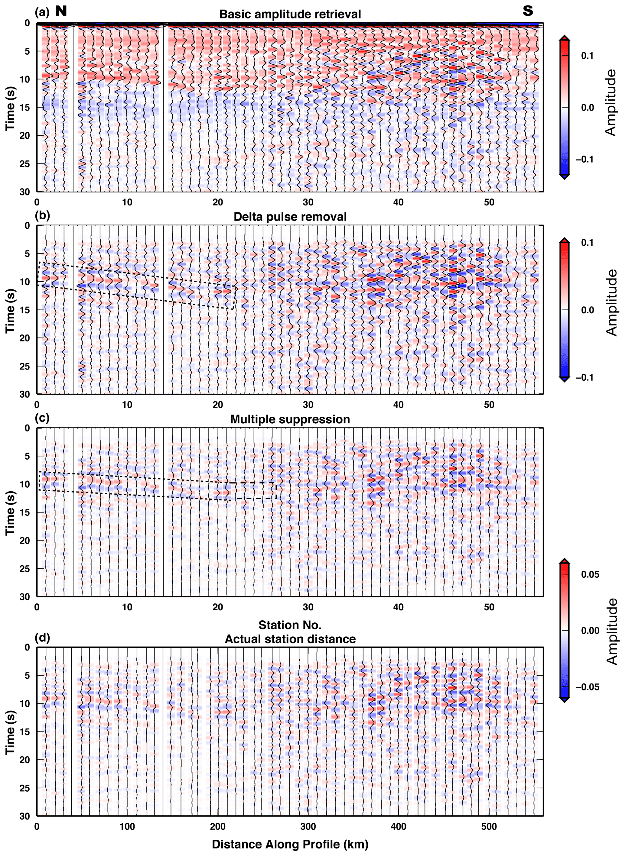
Figure 2 Steps of the GloPSI processing on the ensemble of 64 events listed in Table T1. (a) Basic amplitude retrieval, (b) delta pulse removal, (c) multiple correction and static correction, (d) amplitudes displayed according to the station distance along the north–south direction. Blue–red–blue triplet is outlined between dashed lines in panels (b) and (c).

Within the GloPSI images, we look for the blue–red–blue triplet (e.g. Ruigrok and Wapenaar, 2012) as a marker of a positive impedance contrast (increasing velocity with depth). The Moho is imaged as a triplet signature with a red (positive) signal in the centre and the typical two side lobes of the wavelet creating such a characteristic blue–red–blue feature. We computed the GloPSI response for 100 bootstrapped sets of events (for both cases of including 64 and 27 events). The results have been used to estimate the mean and standard deviation of the amplitudes associated with the images and are shown in Fig. 3 for the 64 events and in Fig. S9 for the 27 events. The three panels in both Figs. 3 and S9 display the SD as a percentage of the maximum amplitude of the relative panels in Figs. 2 and S8. In both figures the northernmost 30 stations show smaller standard deviation values, meaning that the autocorrelated traces are more similar to each other for this part of the transect, while in the southern part of the transect the traces have larger variability.

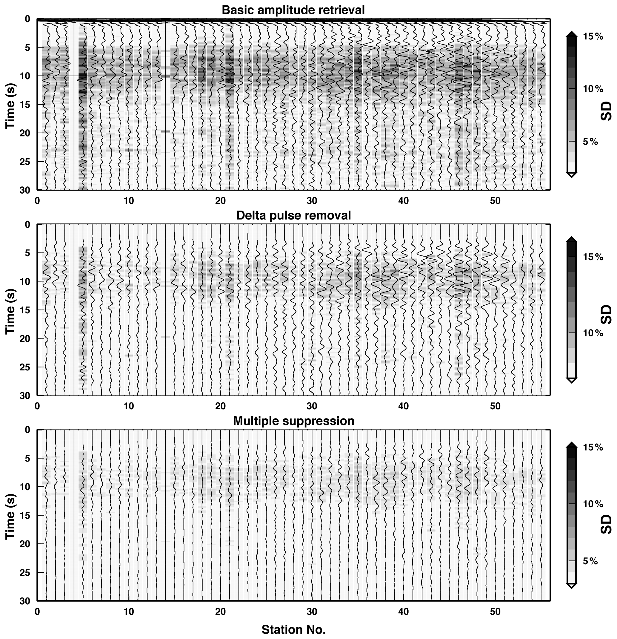
Figure 3 Standard deviation calculated over 100 samples generated by bootstrapping events ensembles by the pool of 64 events (Table 1). Mean wiggles are displayed on top of the SD. The SD for times larger than 15 s is very low due to the absence of strong reflectivity in this time range.

Figure 4 shows the depth-migrated GloPSI results along the EASI profile for (a) the subset of 27 teleseismic sources and (b) the entire dataset (64 teleseismic sources). The two migrated images are quite similar, despite the large difference in input. This gives confidence that these images mostly show receiver-side reflectivity, and most of the cross-terms due to source-side reverberations (SSRs) have been suppressed. Remnant SSR artifacts can be noticed by features that are stronger in Fig. 4a than in Fig. 4b and marked at depth between 65 and 85 km (area 1 and 2, Fig. 4a). These features are disappearing in the northern part of the profile (area 1) and decreasing in amplitude in the southern part of the profile (area 2, Fig. 4b). This shows that adding more phases with different SSRs simply helps in unveiling the receiver-side structure.

Below the Alps (southern part of the profile, area 2 in Fig. 4) not much difference can be noted between the two migrated images. Hence, also at larger depths, both images are already dominated by receiver-side reflectivity. Nevertheless, a part of the imaged amplitudes at larger depth is spurious. In a complex scattering environment like the Alps, there could, for example, be P–S conversion on steep reflectors that end up at the zero-offset response. Also the multiple elimination scheme would be less successful below the Alps where a local 1D assumption poorly holds. With the underlying assumption that only primary P-wave reflections is retrieved, these conversions are then wrongly imaged. We decide to use the image obtained with 64 events (Fig. 4b) for the interpretation.

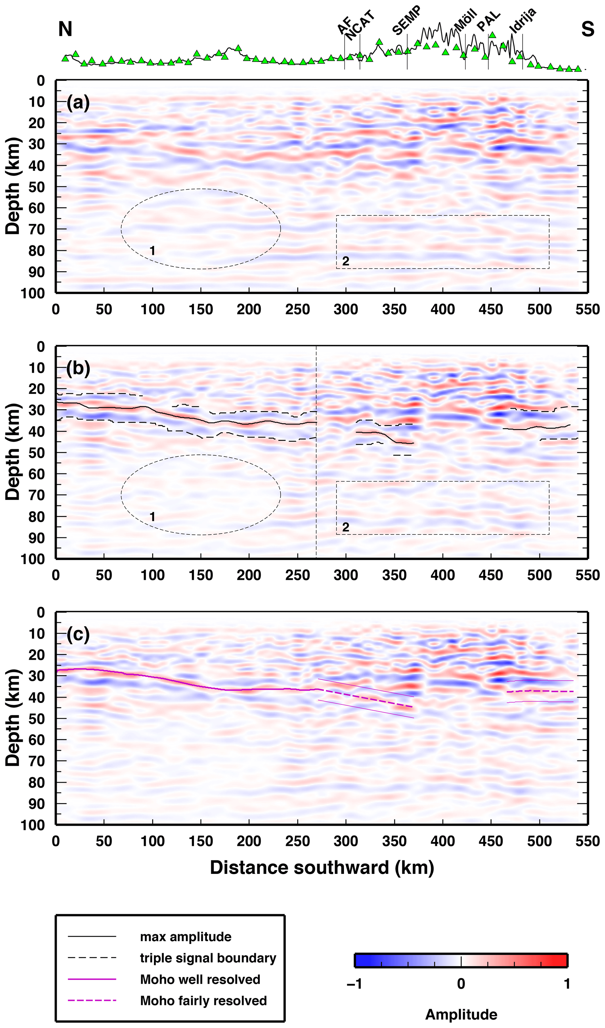
Figure 4 Reflectivity images of the crust and upper mantle along EASI; in the background the interpolated figure (bilinear interpolation), in which blue–red–blue triplet marks the presence of a positive interface (i.e. an increasing impedance contrast with depth). (a) Depth-migrated GloPSI image generated by using 27 events. (b) Depth-migrated GloPSI image generated by using 64 events. The black solid line marks the maximum amplitude within the blue–red–blue triplet; the black dashed line marks the upper and lower boundary of the triplet; features 1 and 2 are described in the text. (c) Background same as (b); solid and dashed purple lines show the picked Moho depths reported in Table 2.

In the migrated image in Fig. 4b, we pick the maximum amplitude (within the blue–red–blue triplet) in the 0–270 km section of the profile for the 64 events (Fig. 4b). We then smooth this interface for a 50 km Fresnel zone for deriving the Moho topography (Fig. 4c). In Fig. 4c also marked is a poorly resolved section of the Moho at the southernmost end. The relatively strong amplitude signals in the crust are nearly identical for either 64 events (Fig. 4b) or 27 events (Fig. 4a) and, therefore, can only be attributed to reflectivity beneath the receiver array. Note that while these moderate to strong amplitude signals of relatively short length (up to 50 km) above the Moho signal are rather common in GloPSI results (e.g. Ruigrok and Wapenaar, 2012). While they are visible all along the EASI profile, beneath the Alps (from profile distance 300 to 520 km) they dominate the image from the top of the crust to where we would expect the Moho based on previously published CSS data (Yan and Mechie, 1989). The difference in the image of these “crustal features” between profile distance 0 and 300 km (Bohemian Massif and northern Alpine Foreland) and below the Eastern Alpine orogen suggests the signals represent at least in parts internal crustal structure.

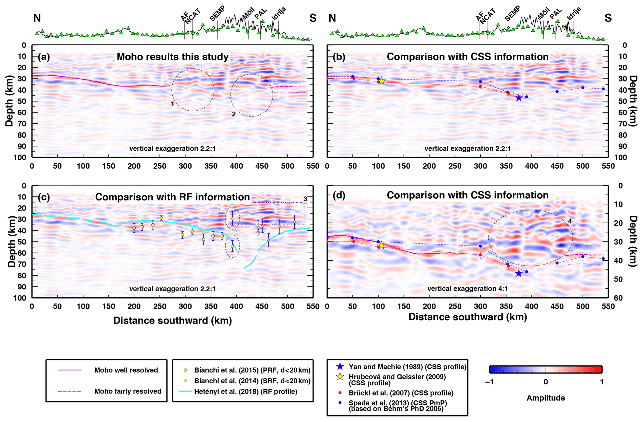
Figure 5 Reflectivity images of the crust and upper mantle along EASI; in the background the interpolated figure as in Fig. 4b. (a) Moho topography beneath the northern Alpine Foreland and the Alps as detailed by results of this study. The subhorizontal and gently dipping Moho is well imaged by our global-phase interferometry, but the typical Moho signal disappears beneath the central parts of the Eastern Alps (features 1 and 2). (b) Comparison with CSS information documenting the generally good correlation between our new Moho results and previous information on crustal thickness outside the Alps. (c) Comparison with RF information where we evidence the co-location of the high reflectivity of crust and the detected anisotropic layer (feature 3). (d) Comparison with CSS information in an enlarged version allows highlighting more detail, and it reveals a nearly perfect correspondence with the PmP model (Behm, 2006; Spada et al., 2013) in the north and an equally good correspondence with the refraction seismic model (Brückl et al., 2007) in the southern part of the foreland. The strong reverberation directly beneath the Alps (4) documents the complex internal crustal structure of the orogen.

4 Discussion

The Moho GloPSI results obtained in this study are documented as a migrated image in Fig. 4c and compared with published information about the Moho along the EASI transect in Fig. 5. In the GloPSI image we notice a clear divide between two domains along the EASI transect. The northern part of the profile (0 to 270 km, possibly 300 km distance along the profile, Fig. 4b) is characterized by low-amplitude reflectors within the crust and one pronounced feature (both in amplitude and length) that can univocally be related to the Moho interface above the uppermost mantle lithosphere that is nearly transparent. The southern part of the profile instead (south of about 300 km) is characterized by high-amplitude reflectivity within the whole crust. The observed alternation of positive and negative phases may suggest the presence of a complex velocity structure with several interfaces of strong velocity discontinuities. In Fig. 5 we included the information from several CSS studies (Fig. 5b and d) and from RF (Fig. 5c) studies. In particular, the CSS profiles analysed by Hrubcová and Geissler (2009) and by Yan and Mechie (1989) are crossing the EASI profile at 110 and 375 km respectively, and they provide two reference points for the Moho depth (stars in Fig. 5b, d). We compare our image also with the refraction seismic model by Brückl et al. (2007) and the Moho depths from the study of Spada et al. (2013), which combined the published CSS profile results with well-resolved Moho depths based on PmP wide-angle reflections (from Behm, 2006). Our results are in good agreement with the CSS profile model by Brückl et al. (2007) along the profile distance 100 to 270 km (see depth-enhanced Fig. 5d). The study of Hrubcová et al. (2005) documented a layer of anomalously high velocity of 7.0 km/s (for the Bohemian Massif) regionally varying in thickness up to 12 km above the Moho. This layer, if taken into account in the depth migration of the GloPSI image, would shift the retrieved Moho towards shallower depth, and closer to the Moho of Spada et al. (2013). Our results beyond profile distance 270 km are difficult to interpret; all available CSS information calls for a distinct increase in the dip of the Moho exactly beneath the northern Alpine front at 300 km profile distance. For further comparison, in Fig. 5c, we plot on top of our GloPSI image the punctual measurements of the Moho depth obtained by depth-migrated S–RF (Bianchi et al., 2014) and by the Zhu and Kanamori (2000) analysis (Zhu and Kanamori, 2000) of P–RF (Bianchi et al., 2015) that were retrieved from stations located within 20 km distance from EASI. We also compare our image with the Moho topography obtained by Hetényi et al. (2018b) with pre-stack migration (PSM) of P–RF along EASI. Our results and the results by Hetényi et al. (2018b) show good agreement from the northern end of the profile to 150 km distance. In this part of the profile, the signals both from RF and GloPSI are clear (Fig. 5c) and we can, therefore, infer the presence of a strong impedance contrast across the Moho. In combination with the results shown in Fig. 5b we conclude the Moho is well imaged univocally by all methods in this northernmost section. Between 150 and 270 km profile distance we notice the divergence between our GloPSI Moho image and results presented by Hetényi et al. (2018b) (Fig. 5c). The laterally varying differences in depth of the Moho might be caused either by errors in the crustal velocity estimates used for depth migration or by the presence of several crustal or mantle features that deviate from being horizontally layered. Considering the Moho results of the refraction seismic profile Alp01 (Brückl et al., 2007) that are rather well resolved in this region, the latter seems unlikely. In the southernmost part of the profile (400 to 550 km distance), the steep northward dip of the Adriatic Moho interpreted by PSM imaging (Fig. 5c) is not seen by our results. The depth-migrated RFs do not show a clear feature in this part of the profile, and the model used for the depth migration does not take into account high lower crustal velocities (Fig. S10); anyways, we should also consider that the GloPSI method is suitable for identifying sub-horizontal to gently dipping interfaces and therefore might fail in imaging such a described inclined interface. In this part of the profile (440 to 550 km distance), the Moho estimates from single-station analysis have been derived by depth-migrated S-wave RF (Bianchi et al., 2014). The low frequency of the used S wave is the reason for the large errors associated with these depth estimates, and from such an analysis it would not be possible to separate the contribution of more than one impedance contrast at depth. Moreover, the two different depths inferred from the same station (circled in Fig. 5c) suggest the presence of several impedance contrasts in the crust for this section of the profile. As a last comparison, previous RF studies on crustal structures (Bianchi and Bokelmann, 2014) located anisotropy at the mid-lower crust, extending from the Salzach–Ennstal–Mariazell–Puchberg (SEMP) fault southward (feature 3 in Fig. 5c). From the GloPSI, in this area (SEMP and southward, lower crust) we see a high reflectivity pattern. The co-located high reflectivity (from GloPSI) and anisotropy (from RF) are possibly due to the same physical reasons (e.g. layering or imbrication), which contribute to fading the Moho signal beneath the Alps. In summary, the GloPSI results nicely complement the published results along the EASI transect derived from CSS and RF studies (Fig. 5). As discussed above, the three seismic methods exhibit different strength and limitations, but they are all particularly sensitive to the first-order velocity discontinuity that represents the crust–mantle boundary. The correspondence of the Moho depth obtained by the three different seismic methods in the northernmost 150 km of the profile suggests a crust and a Moho in this part of the northern Alpine Foreland that correlates well with the models for the continental crust proposed by Mueller (1977) and Musacchio et al. (1998) and with the crustal models published for the northern foreland further west (e.g. Ye et al., 1995). Our GloPSI results and those published from CSS studies continue to correspond well further south beneath the Molasse basin (to profile distance 270 km and possibly 300 km) to the northern limits of the Eastern Alps. In this section of the transect, we note that the RF results show significant lateral variations in depth and also differences between the two RF studies. Since the study of Hetényi et al. (2018b) is confined to the temporary stations of the EASI profile and the study of Bianchi et al. (2015) punctually samples a wider region including permanent stations, these differences possibly reflect lateral velocity variations in the crust beneath the Molasse basin and further south in the northernmost Alps. Moreover, Hetényi et al. (2018b) use the regional V_p and V_s model from Molinari and Morelli (2011) for migrating the Moho Ps conversions. We instead use a transect-specific V_p model (Brückl et al., 2007), which is much more detailed and reliable for the EASI transect.

Our GloPSI results document a complex crustal structure beneath the Eastern Alps. While this complexity prevents us from further interpreting any signals south of profile distance 300 km, a number of studies have proposed models of the deep structure beneath the high Eastern Alps east of 13^∘ E. As Fig. 5b and c show, these models differ greatly in the estimated Moho topography across the plate boundary. With the exception of the CSS longitudinal profile by Yan and Mechie (1989), all studies suffer from limitations of the method or the dataset, or both, to reliably resolve the crustal structure and Moho topography in this most interesting region. In the Eastern Alps, the number of CSS profiles and experiments for academic reasons is limited, and the restoration of subsurface geometries yields ambiguous results due to the 3D characteristics of the orogenic root. Anyways, thanks to the recent passive seismic experiments (Hetényi et al., 2018a, b; Heit et al., 2021), the number of data acquired in the area is significantly increased, leading to new images and interpretations, which are overcoming the difficulty of illuminating the deep crustal structures and might suggest simpler interpretations (i.e. Sadeghi-Bagherabadi et al. (2021) draw a flat and continuous Moho at about 50 km depth in the gap area).

5 Conclusions

We applied global-phase interferometry to data collected by the passive seismic deployment EASI, which crosscuts the Eastern Alps along a 550 km long north–south profile. Inferring the crustal thickness and the nature of the Moho below the Alpine crests has been challenging in the last decades and has led to different and often opposing interpretations. In this work, we have the opportunity to review and compare previous information on Moho depth, aside from producing a new image of the crust. From north to south we can follow the different responses of the crust to the different imaging techniques (GloPSI, CSS and RF). In the northernmost part of the profile we obtain consistent depth estimates, which suggest a very simple crustal structure and a high impedance contrast at the Moho. Between 100 and 270 km along the profile, we observe diverging Moho depth estimates, which might be due to an anomalously high-velocity lowermost crustal layer, known to exist below parts of the Bohemian Massif, and/or to lateral variations or local topography of the Moho interface. Between profile distance 270 and 300 km, the GloPSI does not deliver a clear image of the Moho, due to the southern dip of the European Moho. The segment of the profile between 300 and 550 km is the most controversial and the one hosting the long-debated and unclear crust–mantle boundary. The application of the GloPSI technique did not constrain the Moho topography immediately beneath the Eastern Alps, but it did image the complex lower crustal structure. To univocally image the crust–mantle transition below the Eastern Alps, we further need to address this area by integrating and combining several seismic methods.