the Creative Commons Attribution 4.0 License.
the Creative Commons Attribution 4.0 License.
 | 02 Jun 2021
Regional centroid moment tensor inversion of small to moderate earthquakes in the Alps using the dense AlpArray seismic network: challenges and seismotectonic insights
Simone Cesca
Sebastian Heimann
Peter Niemz
Torsten Dahm
Daniela Kühn
Jörn Kummerow
Thomas Plenefisch
The Alpine mountains in central Europe are characterized by a heterogeneous crust accumulating different tectonic units and blocks in close proximity to sedimentary foreland basins. Centroid moment tensor inversion provides insight into the faulting mechanisms of earthquakes and related tectonic processes but is significantly aggravated in such an environment. Thanks to the dense AlpArray seismic network and our flexible bootstrap-based inversion tool Grond, we are able to test different setups with respect to the uncertainties of the obtained moment tensors and centroid locations. We evaluate the influence of frequency bands, azimuthal gaps, input data types, and distance ranges and study the occurrence and reliability of non-double-couple (DC) components. We infer that for most earthquakes (Mw≥3.3) a combination of time domain full waveforms and frequency domain amplitude spectra in a frequency band of 0.02–0.07 Hz is suitable. Relying on the results of our methodological tests, we perform deviatoric moment tensor (MT) inversions for events with Mw>3.0. Here, we present 75 solutions for earthquakes between January 2016 and December 2019 and analyze our results in the seismotectonic context of historical earthquakes, seismic activity of the last 3 decades, and GNSS deformation data. We study regions of comparably high seismic activity during the last decades, namely the Western Alps, the region around Lake Garda, and the eastern Southern Alps, as well as clusters further from the study region, i.e., in the northern Dinarides and the Apennines. Seismicity is particularly low in the Eastern Alps and in parts of the Central Alps. We apply a clustering algorithm to focal mechanisms, considering additional mechanisms from existing catalogs. Related to the N–S compressional regime, E–W-to-ENE–WSW-striking thrust faulting is mainly observed in the Friuli area in the eastern Southern Alps. Strike-slip faulting with a similarly oriented pressure axis is observed along the northern margin of the Central Alps and in the northern Dinarides. NW–SE-striking normal faulting is observed in the NW Alps, showing a similar strike direction to normal faulting earthquakes in the Apennines. Both our centroid depths and hypocentral depths in existing catalogs indicate that Alpine seismicity is predominantly very shallow; about 80 % of the studied events have depths shallower than 10 km.
- Article
(19510 KB) - Full-text XML
-
Supplement
(1604 KB) - BibTeX
- EndNote


The Alpine mountains and surrounding areas are known for their complex tectonic setting with a highly heterogeneous lithospheric structure (e.g., Handy et al., 2010, 2015; Schmid et al., 2004; Hetényi et al., 2018). The mountain range was tectonically shaped by the interaction of the Adriatic microplate and the European plate in several stages of convergence between Europe and Africa (e.g., Schmid et al., 2004, 2008; Handy et al., 2010; Hetényi et al., 2018). Geological studies show that the Adriatic plate is the upper plate in the subduction of the Alpine Tethys in the Alps, while it is the lower plate of the thrust systems in the Apennines and the Dinarides (e.g., Schmid et al., 2008; Handy et al., 2015). The terranes of the Mesozoic Tethys ocean between Europe and Africa were compressed, rotated, faulted, and stacked during the Alpine orogenesis (e.g., Handy et al., 2010). Along a distance of approximately 700 km between NW Italy and Slovenia, the Northern Alps and the Southern Alps are separated by the Periadtriatic line or fault system (e.g., Handy et al. (2005); see also Fig. 1). Reversals in the subduction polarities have been proposed at the transition to both the Apennines and the Dinarides, while the geometry and orientation of the slab is still controversial (e.g., Hetényi et al., 2018; Handy et al., 2010, 2015; Mitterbauer et al., 2011; Schmid et al., 2004). GPS measurements show that the Adriatic microplate is rotating counterclockwise relative to Europe around an Euler pole located in the Western Alps or western Po plain (D'Agostino et al., 2008; Weber et al., 2010). Velocity anomalies in the crust and the upper mantle reflect the complexity of the crustal structure and the geodynamic setting (e.g., Diehl et al., 2009; Fry et al., 2010; Molinari et al., 2015; Kästle et al., 2018; Lu et al., 2020; Qorbani et al., 2020).
Seismic activity across the Alps is typically characterized by low- to moderate-magnitude earthquakes. However, large damaging earthquakes have occurred in the past, such as the 1356 Basel earthquake (Meyer et al., 1994) or the 1976 Friuli earthquake (Mw 6.45, Poli and Zanferrari, 2018). Recent seismic activity in the eastern Southern Alps is caused by the N–S convergence (2–3 mm yr−1) between the Adriatic Plate and Eurasia, which is accommodated by the ENE-trending, SSE-verging thrust front of the eastern Alps and by the NW–SE-trending right-lateral Dinaric strike-slip fault systems in western Slovenia (Moulin et al., 2016; Poli and Zanferrari, 2018). The wider Alpine region, including parts of the Dinarides and the Apennines, stretches across Switzerland, Austria, Liechtenstein, France, Italy, Germany, Slovenia, and Croatia. Most of these countries have national earthquake observatories, research institutes or universities that routinely monitor the regional seismicity. The Swiss Seismological Service (SED) and the Slovenian Environment Agency (ARSO) provide annual reports containing mainly first-motion-based focal mechanisms (e.g., Diehl et al., 2018; Ministrstvo za okolje in prostor Agencija RS za okolje, 2020), while for example INGV (Italy), GEOFON (Germany), EM-RCMT (European-Mediterranean Regional Centroid-Moment Tensors; Pondrelli, 2002), SISMOAZUR (France), and GCMT (Lamont-Doherty Earth Observatory of Columbia University, USA) provide moment tensor (MT) solutions in online bulletins for magnitudes above 3.5 or larger (see the data and code availability section for more information).
The region can be characterized by compartments with varying tectonic movement in close proximity, as described by many studies of local seismic activity. Focal mechanism in the SW Alps indicate predominantly N–S-to-NNW–SSE-striking normal faulting (e.g., Nicolas et al., 1998; Sue et al., 2000), while in the W Alps strike-slip earthquakes have been observed and explained as a consequence of regional NW–SE compression and NE–SW extension (Maurer et al., 1997). In the central Alps, Marschall et al. (2013) observe strike-slip faulting in central Switzerland. NW–SE-striking normal faulting is reported for SE Switzerland (e.g., Marschall et al., 2013; Diehl et al., 2018). Reiter et al. (2018) provide focal mechanism solutions from P (primary) and S (secondary) polarities and amplitude ratios for the Central to Eastern Alps. They report strike-slip mechanisms and oblique strike-slip mechanisms in the Brenner–Inntal transfer zone (see Brenner and Inntal fault in Fig. 1), and normal faulting is seen with a strike direction parallel to the Giudicarie fault system. Within this fault system, E–W-to-NE–SW-striking thrust faulting with strike-slip components were described by Viganò et al. (2008). The Italian MT dataset provides extensive mechanisms for N Italy. Within the Lake Garda region and in the eastern Southern (eS) Alps close to Friuli thrust faulting with ENE–WSW to ESE–WNW strike direction is dominant (Pondrelli et al., 2006; Anselmi et al., 2011; Bressan et al., 1998). East of Friuli and in the northern Dinarides, both (oblique) thrust and strike-slip faulting is observed (Pondrelli et al., 2006; Moulin et al., 2016). This overview is not complete by far but provides a small glimpse into the complex seismic and tectonic activity that is not simply dominated by the main active deformation fronts at the southern and northern margin of the Alps but that also occurs in smaller fault systems across the entire region.
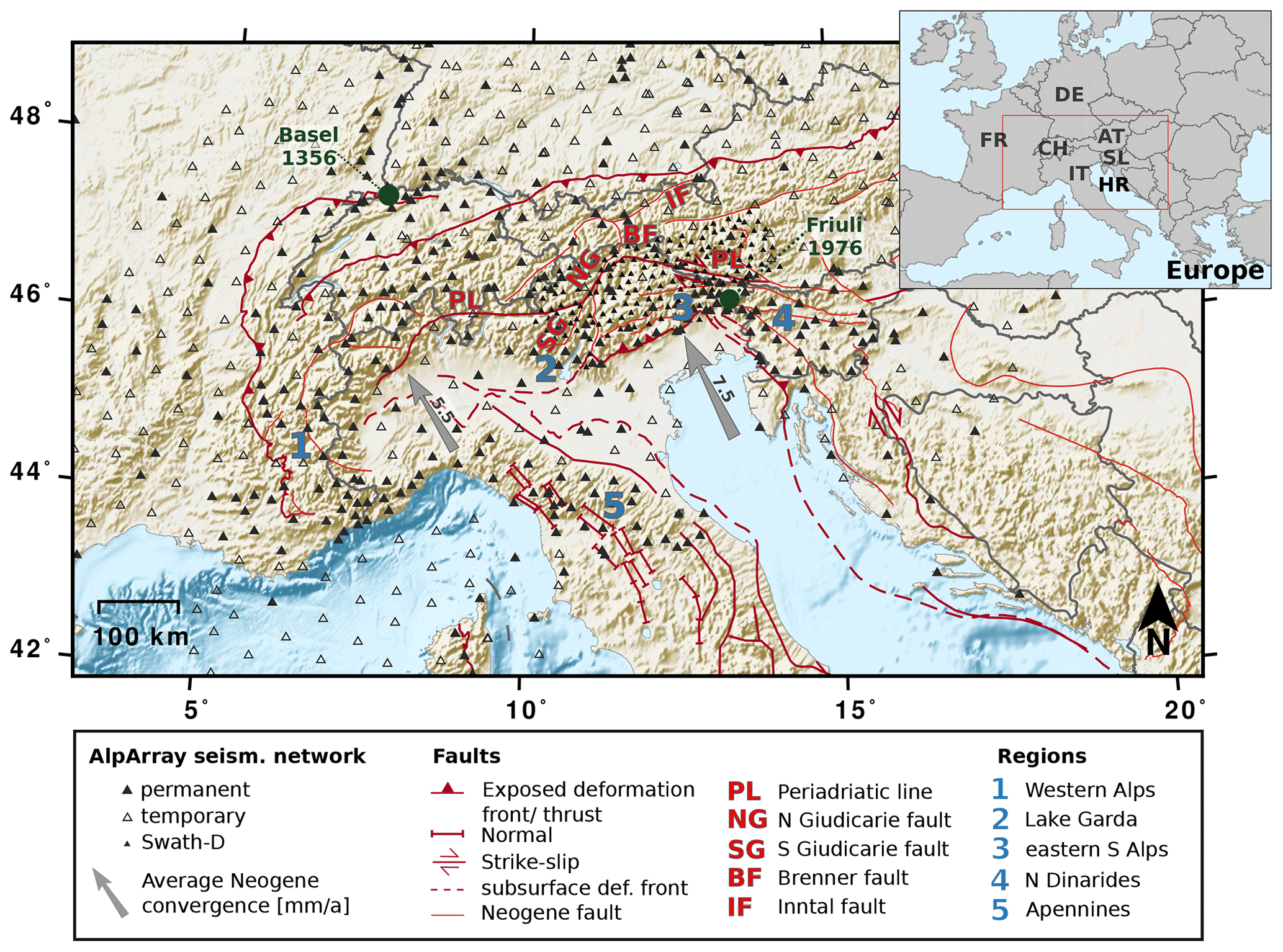
Figure 1Study area and AlpArray seismic network. Subregions that are discussed in greater detail in this study are numbered. Arrows indicate average Neogene (20–0 Ma) Adria–Europe convergence rates from Le Breton et al. (2017). Exposed and subsurface faults simplified from Schmid et al. (2004, 2008), Handy et al. (2010, 2015), and Patacca et al. (2008). Topographic data from SRTM-3 (Farr et al., 2007) and ETOPO1 (Amante and Eakins, 2009) datasets. The inset shows the location of the study area in Central Europe (red rectangle): FR is France, DE is Germany, IT is Italy, SW is Switzerland, AT is Austria, SL is Slovenia, and HR is Croatia.
To study the orogenesis of the Alps and related processes like recent seismic activity, mantle dynamics, plate motion, and surface processes, the AlpArray initiative was established. In this initiative, more than 35 European institutes joined resources to operate the AlpArray Seismic Network (AASN) (Hetényi et al., 2018), consisting of more than 600 temporary (AlpArray Seismic Network, 2015) and regional permanent stations with an average spacing of <60 km (Fig. 1). For comparison, in summer 2011, before the AASN planning period started and first additional permanent stations were set up, there were 234 stations in the same area (Hetényi et al., 2018). The AASN is complemented by the dense Swath-D network in the eastern Alps (Heit et al., 2017). The permanent stations of the AlpArray are part of existing European regional networks (RD, GU , CZ, ST, G, CH, OE, MN, HU, GE, RF, FR, IV, BW, SX, NI, TH, OX; see data and code availability). The dense AASN allows for studying regional seismicity in new, greater detail and provides the opportunity to perform centroid moment tensor (CMT) inversions with a constant station coverage over the entire region. In contrast, many of the previous studies focus on specific regions or seismic sequences within the Alps, and therefore do not provide a broad overview. Furthermore, many of these studies relied on first-motion polarities. First-motion-based approaches can be used even for small earthquakes when no surface wave energy is observed. However, the obtained mechanism is only representative for the very first moment of the fracturing process. This might introduce discrepancies when comparing first-motion solutions to MT solutions (Scott and Kanamori, 1985; Guilhem et al., 2014). The instability of take-off angles of shallow earthquakes may introduce significant errors in the polarity readings (Hardebeck and Shearer, 2002). Additionally, first-motion solutions of small earthquakes are often only based on few polarities, which makes it difficult to assess uncertainties.
Despite the limited resolution, first-motion polarity approaches are often used in the Alps, where MT inversion is particularly challenging. First, earthquake magnitudes are generally small to moderate, requiring waveform modeling at relatively high frequencies and local distances. Furthermore, structural heterogeneities, site effects, and topographic effects hinder full waveform MT inversions based on 1-D velocity profiles when considering frequencies above 0.1 Hz. Signal-to-noise ratios (SNR) vary significantly across the region due to densely populated areas and environmental conditions (weather and wind, rivers, rock falls, avalanches, etc.). Each study or observatory reporting focal mechanisms uses different inversion tools, input data, and distance and frequency ranges. Furthermore, uncertainties are not routinely discussed, which makes it difficult to evaluate published solutions. Uncertainties can be assessed, e.g., by performing a grid search over parameters like strike, dip, rake, and depth (Stich et al., 2003; Cesca et al., 2010) or using independent bootstrap chains in the inversions with varying weighting of the input data from different stations (e.g., Heimann et al., 2018; Kühn et al., 2020, and this study). The latter approach provides uncertainties of all inversion parameters (e.g., MT components, centroid location) and helps to identify trade-offs between these parameters.
Studies of focal mechanisms in the Alps have mainly considered double-couple (DC) solutions. Here, based on the dense seismic network, we also attempt to consider non-DC components. The decomposition of the moment tensor allows for studying the seismic source in more detail, including not only pure tectonic dislocations represented by the DC but also volumetric changes and tensile faulting (e.g., Vavryčuk, 2015).
In this study, we predominately target small to moderate earthquakes (Mw>3.0) that occurred in the Alps or surrounding areas between January 2016 and December 2019, based on the operation time of most of the temporary broadband stations of the AASN. While the temporarily densified network provides a great amount of input data to the single MT inversions, the short time span limits the number of observed earthquakes. We test various setups and input types to establish workflows for a homogeneous and consistent list of MT solutions for the Alps (see Supplement). We attempt to lower the magnitude threshold for inversions compared to routinely reported solutions by optimizing the used methods and by combining different input data types (e.g., time domain full waveforms and frequency domain amplitude spectra). Using the AASN and the bootstrap inversion framework Grond (Heimann et al., 2018; Dahm et al., 2018; Kühn et al., 2020) allows for determining the most suitable setups for source inversions of small to moderate earthquakes within the study area.
After an introduction into the inversion method, we describe the methodological tests that were performed to assess inherent methodological uncertainties. At the same time, we propose guidelines for MT inversion of small to moderate earthquakes in complex tectonic settings. Subsequently, we present the MT solutions that were obtained for the Alpine region and discuss these with respect to mechanisms, spatial patterns, and centroid depths. We discuss different tectonic areas in the Alps systematically, including observations of seismicity, faulting mechanisms, and GNSS deformation data.
2.1 Moment tensor inversion using Grond
We use the open-source software Grond for MT inversions (Heimann et al., 2018; Kühn et al., 2020). In a Bayesian bootstrap-based probabilistic joint inversion scheme, solution uncertainties are retrieved along with the best-fitting CMT solution (see also Dahm et al., 2018). We simultaneously invert for the six independent moment tensor components, for the seismic moment, for the centroid location, and for the origin time. The objective function is set up in a flexible way to combine different input data types as a weighted sum. In our study, we use combinations of time domain full waveforms, time domain cross-correlations, and frequency domain amplitude spectra as an input for the inversion. Following the studies of Zahradník and Sokos (2018) and Dahal and Ebel (2020), we implemented envelopes of time domain waveforms. The misfits of the different input data are combined using an L1 or L2 norm. We assign the same weighting to each input data type. The misfit values of single stations within one input data type group are weighted to account for different epicentral distances (Heimann, 2011). Without applying such a weighting, summed misfits are always dominated by the closest stations which have the highest amplitudes. In the case of using time domain full waveforms or cross-correlation fitting procedures, we allow for small time shifts to compensate for errors in the velocity models. To avoid the mismatching of phases, these time shifts were set to be well below a quarter of the dominant wavelength. Time shifts are regulated by a penalty function with an empirically chosen maximum of 0.05.
Precalculated Green's function databases are used for rapidly computing synthetic data (Heimann et al., 2019). In our case, we used regional velocity profiles from the CRUST2.0 Earth model database (see https://igppweb.ucsd.edu/~gabi/crust2.html, last access: June 2020; Bassin et al., 2000), which we choose according to the earthquake epicenter location. The Green's function databases were calculated with the orthonormal propagator algorithm QSEIS (Wang, 1991). Grond selects the appropriate time window, corrects the recorded waveforms for the instrument response, and rotates to ZRT coordinate system. Filters are applied and, if specified, waveform attributes as spectra or envelopes are calculated. The inversion is performed in parallel bootstrap chains (here, 100 for normal inversions and 500 for method testing), where individual bootstrap weights are applied to the single-station-component input data type combinations. Bootstrapping is applied for two reasons. Firstly, to avoid distortions due to a few high misfit values resulting from a low SNR at single stations, incorrect transfer functions, or malfunctioning stations. Secondly, the bootstrap chains are used to access model parameter uncertainties and trade-offs between the inversion parameters. Each bootstrap chain performs an entirely independent optimization. Along with the best solution with the lowest misfit, Grond provides a defined number (here, 10) of best solutions of each bootstrap chain, which we call the ensemble of solutions.
Figure 2 presents a selection of plots provided by the inversion software to assess the solution robustness, in this case for the 14 June 2019 thrust-faulting earthquake in northern Italy (Mw 3.9). Figure 2a shows the fuzzy MT, which is an illustration of the MT uncertainty. It is composed of the superimposed P radiation pattern of the ensemble of solutions from the bootstrap chains. If the variability of the ensemble solutions is small, and hence the uncertainties are small (as seen here), the fuzzy plot has clearly separated black and white quadrants. The red lines indicate the solution with the lowest misfit. Other plots show the station distribution (Fig. 2b) and the decomposition of the best deviatoric MT solution into the DC and the CLVD component (Fig. 2c). Figure 2d shows the distribution of the centroid locations obtained from all ensemble solutions, and Fig. 2e depicts the resolution of the six independent MT components in the form of probability density functions. As is typical for shallow events inverted using surface waves, the mnd and med components are not as well resolved as the other components (Cesca and Heimann, 2018; Bukchin et al., 2010; Valentine and Trampert, 2012). Finally, Fig. 2f shows examples of waveform and frequency spectra fits of Z, R, and T component traces at three stations.
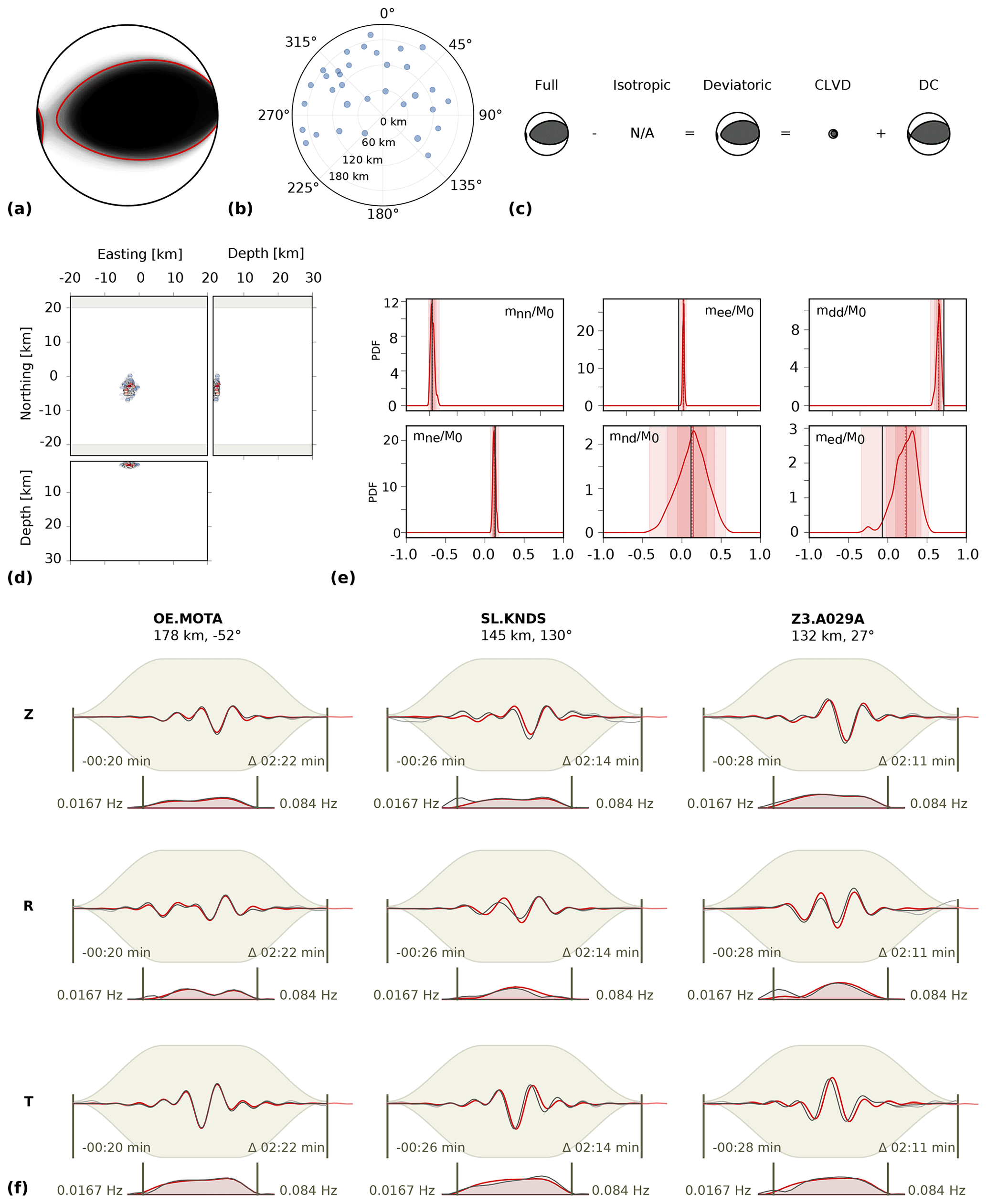
Figure 2Example of an MT inversion result, 14 June 2019, Mw 3.9, NE Italy. (a) Fuzzy beach ball illustrating the MT solution uncertainty. (b) Station distribution around the epicenter. (c) Decomposition of the best MT solution into DC and CLVD component. (d) Resolution of the centroid depth, easting, and northing relative to the starting position. (e) Probability density functions (PDFs) showing the resolution of the six independent MT components mxy normalized by the seismic moment M0. (f) Examples of waveform and spectral fits at three stations and three components. Red and black lines indicate synthetic and recorded waveform data, respectively. The beige-shaded area represents the time window and taper function. Station name, azimuth, and distance to the epicenter are indicated above each column. Numbers within the panels describe the time window and the frequency band.
The selection and joint inversion of waveform attributes can improve the stability and goodness of solutions. In the following, we want to point out advantages and drawbacks of the waveform-based input data types, which are used in the subsequent methodological tests: time domain (TD), frequency domain (FD), cross-correlation, and envelopes.
2.1.1 TD full waveform fitting
In the time domain, the misfit between a selected time window of a seismic trace and a synthetic trace in a defined frequency range is computed as the normalized sum of sample misfits. Time shifts are allowed and regulated with a penalty function. For regional MT inversion, surface waves are commonly considered in full waveform approaches (e.g., Ritsema and Lay, 1995; Minson and Dreger, 2008; Sokos and Zahradnik, 2008; Dahm et al., 2018). The frequency band is magnitude dependent. While at low frequencies effects of the velocity model and topography are minor, at higher frequencies the SNR is usually better. At regional distances, magnitude-dependent frequency bands below 0.1 Hz are often used to consider Rayleigh waves and Love waves, which have particularly simple waveforms at this distance range (Ritsema and Lay, 1995). However, in the case of very shallow sources, the resolution of the mxz and myz components of the MT are limited when using surface waves (Bukchin et al., 2010; Valentine and Trampert, 2012; Cesca and Heimann, 2018, see also Fig. 2). Relying on time domain fitting only, time shifts, noisy data, or distorted amplitudes can hinder finding stable initial inversion solutions. It has proven to be helpful to combine time domain full waveform fitting with other input data types like frequency domain amplitude spectra, which are often less affected by these issues.
2.1.2 FD amplitude spectra fitting
Real-valued amplitude spectra of recorded Love and Rayleigh waves carry all information necessary to resolve the geometry of the MT, while neglecting the phase information and dispersion (e.g., Mendiguren, 1977). This means that two MT solutions with common nodal planes but opposite polarities model the amplitude spectra equally well and that additional information from first-motion polarity readings or time domain waveform fitting is needed to resolve this ambiguity (e.g., Cesca et al., 2010; Heimann, 2011). The misfit is computed as the misfit between amplitude spectra of recorded and synthetic waveforms in a selected frequency range and time window. Compared to fitting full waveforms in the time domain, more conservative, less exact time windows can be selected. Cesca et al. (2010, 2013) propose a multistep approach to stepwise combine the fitting of amplitude spectra and displacement waveforms to subsequently obtain point source parameters, the centroid location, and kinematic source parameters. Compared to full waveform fitting, amplitude spectra inversion methods are less sensitive to trace misalignments and phase shifts resulting from coarse or erroneous velocity models (Cesca et al., 2010, 2013; Domingues et al., 2013). In the subsequent tests, we do not use a stepwise inversion but use amplitude spectra and time domain full waveforms or cross-correlated waveforms simultaneously.
2.1.3 Cross-correlation waveform fitting
In the cross-correlation-based fitting of full waveforms, the amplitudes of recorded and synthetic traces are normalized. The inversion searches for the maximum cross-correlation value for the selected time window in time domain, basically fitting the phase shift (Stähler and Sigloch, 2014; Kühn et al., 2020). Cross-correlations help to constrain the centroid location and centroid time in a joint inversion. We allow for small time shifts, regulated with a penalty function, to compensate for imprecise velocity models. Time shifts need to be small compared to the frequency range in order to avoid mismatching phases. Due to the amplitude normalization, this method is sensitive to patterns in the waveforms, while it is not influenced by gain errors or site effects. Magnitudes cannot be resolved. Cabieces et al. (2020) used cross-correlation fitting in their MT inversion for ocean bottom stations, where absolute amplitudes could not be modeled due to the unknown coupling to the ground. When using cross-correlations to fit time domain waveforms, frequency bands and time windows need to be selected carefully to avoid mismatching phases.
2.1.4 Envelope fitting
In our study, we compute the waveform envelopes by convolving the squared time series using the fast Fourier transform with a Hanning taper. This smoothens and therefore simplifies the waveforms. Hensch et al. (2019) used non-smoothed envelopes in the same inversion routine in combination with amplitude spectra, spectral ratios, and time domain waveforms. Envelopes, especially smoothed ones, are less influenced by small un-modeled time shifts or noisy data compared to full waveforms. Fitting envelopes of seismic waveforms can be helpful in the case of using high-frequency bands, simplified velocity models, and increased noise levels. Zahradník and Sokos (2018) stress that due to the simplification of the waveforms, the results of envelope-based inversions have a limited precision and results need an even more careful inspection of uncertainties and resolution. However, if body waves are considered, envelopes can especially help to constrain P- and S-phase arrivals and thus the centroid time and location. Since the envelopes are based on absolute amplitudes, they need to be combined with a method providing polarity information. Zahradník and Sokos (2018) and Dahal and Ebel (2020) have shown that envelopes can be used to derive focal mechanisms for M<4 events in the case of unfavorable settings like sparse networks, for which full waveform fitting is not feasible. In both studies, the envelopes are combined with P polarities of one or more nearby stations to resolve the polarity ambiguity.
2.2 Methodological tests
We perform methodological tests using recorded seismograms and synthetic data to investigate the resolution capacities, requirements, and limits of MT inversions in the Alpine region. We use subsets of representative earthquakes that occurred between 2016 and 2019 in the Alps. The tests are particularly computationally demanding, as every single inversion of each test is run in 500 bootstrap chains. The number of events in each test depends on the number of tested parameters. The proposed tests can be used as a guideline for assessing the feasibility of MT inversions in other study areas with moderate seismicity.
We benefit from the large seismic network and use more than 80 stations at distances of up to 400 km for the largest events (Fig. 3). For earthquakes with moderate magnitudes between Mw 3.5–3.9, we mostly rely on 20 to 50 stations within a radius of 200 km. The number of available stations depends on the magnitude and the epicenter location within the network. Furthermore, the SNR and quality of the individual stations is variable in time and space. Before the inversions, we applied the toolbox AutoStatsQ to identify seismic stations with misorientations, metadata errors, or gain problems (Petersen et al., 2019).
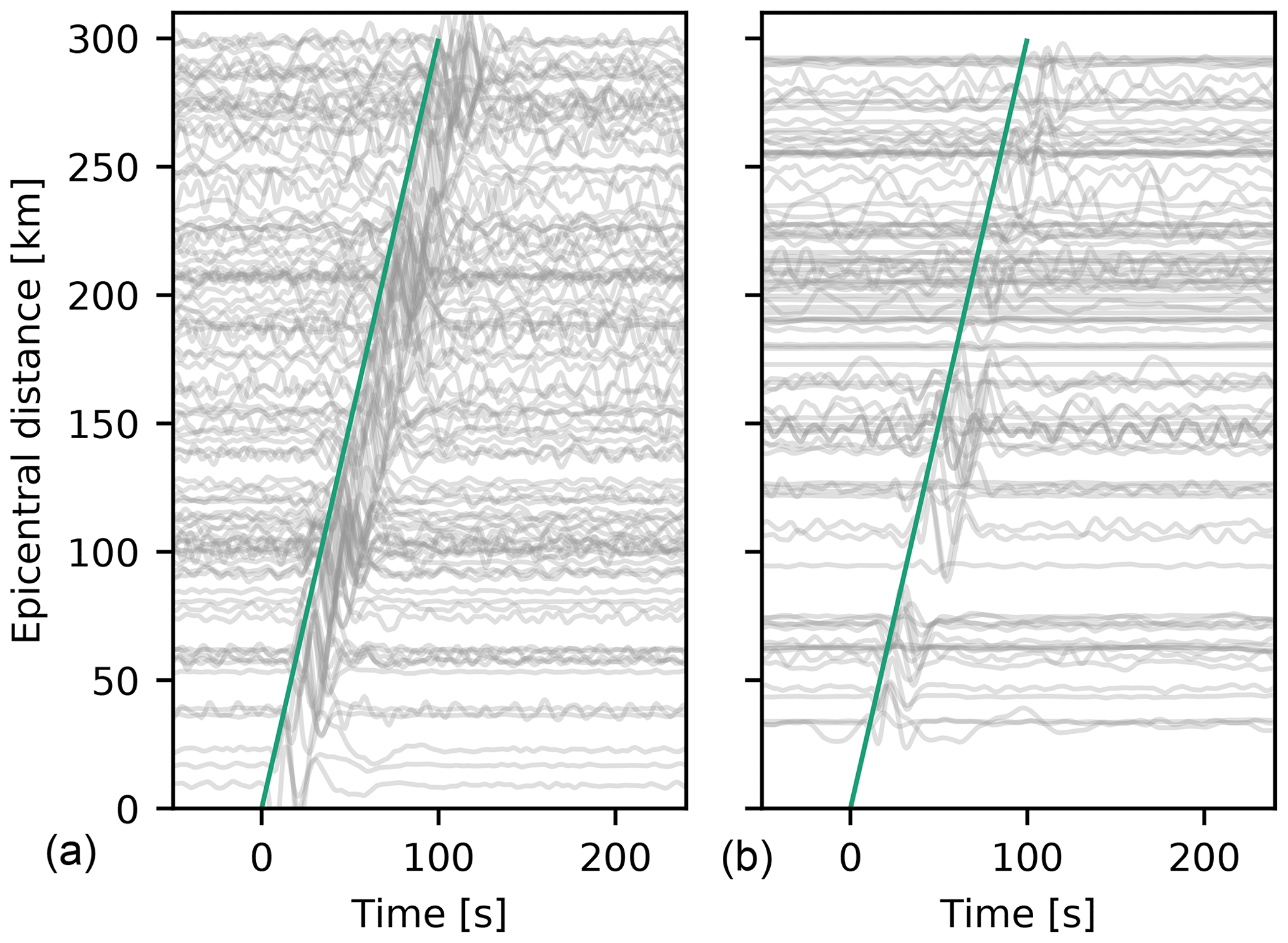
Figure 3Vertical component seismograms of permanent AASN stations, sorted by distance: (a) 6 March 2017, Mw 4.1, Switzerland; (b) 27 October 2017, Mw 3.6, France. Time is in seconds after origin time. Waveforms are bandpass-filtered between 0.02 and 0.07 Hz. Rayleigh waves dominate the seismograms in this frequency range with an average phase velocity of 3 km s−1 (green line).
2.2.1 Double-couple, deviatoric, and full moment tensor inversions
We study the stability and resolvability of non-DC components by performing full, deviatoric, and pure DC MT inversions for a subset of 32 earthquakes of the AlpArray dataset. We consider these earthquakes representative as they cover a large magnitude range (Mw 3.2–4.2), are distributed across the entire study area, and are comprised of different types of mechanisms. We use a passband of 0.02–0.07 Hz and fit time domain full waveforms and frequency domain amplitude spectra simultaneously. We compared the pure DC, the deviatoric, and the full MT obtained for each earthquake with respect to the fit of the recorded data and to the uncertainties of MT components and centroid locations. Subsequently, we statistically evaluate those solutions, for which a low misfit between synthetic and observed waveforms was achieved with all three inversion types. Four events with Kagan angles > 60∘ between full and deviatoric solutions were removed since they were not well resolved.
The isotropic source component of the seismic moment tensor resolves volumetric changes, including processes like explosions, cavity collapses, fluid movement, or ruptures on nonplanar faults (e.g., Sileny and Hofstetter, 2002; Ford et al., 2009; Miller et al., 1998; Minson and Dreger, 2008). The CLVD component is often described as the residual radiation to the best DC without geological interpretation (Dahm and Krüger, 2014), it is however required for a mathematically complete decomposition (Vavryčuk, 2015). Large CLVD components are often explained by noisy data, a simplified or incorrect velocity model, neglected 3-D wave effects, or insufficient station coverage (e.g., Panza and Saraò, 2000; Cesca et al., 2006) but can also be interpreted physically in combination with an isotropic component of the same sign as a product of tensile faulting (Vavryčuk, 2015). Non-DC components are also used as an indicator of anthropogenic seismicity (Dahm et al., 2013; Cesca et al., 2013; Lizurek, 2017).
Despite frequent geological interpretations which propose fluid movements or tensile processes, various studies show that resolving non-DC components in MT inversions is particularly difficult. Seismic noise and inaccurate Green's functions may result in large non-DC components. Trade-offs between hypocenter location or depth and isotropic component have been observed (e.g., Dufumier and Rivera, 1997; Panza and Saraò, 2000; Křížová et al., 2013; Kühn et al., 2020). Non-DC components must therefore be evaluated carefully with respect to tectonic processes (Lizurek, 2017). Methodological tests based on observed data and synthetic tests can help to identify which non-DC components can be considered statistically significant (see also Panza and Saraò, 2000).
Figure 4a and b show the ratio of DC and non-DC components of the full and deviatoric MT inversions of our test dataset. The deviatoric inversions result in 0 %–40 % CLVD components for 70 % of the events and in CLVD components of >50 % for 19 % of the events. In the case of full MT inversions, we find significant isotropic components of >30 % in the case of one-third of the earthquakes. Figure 4c indicates that the non-CLVD components of the test events scatter significantly. It is clearly visible that many events with shallow depths (dark colors) are located in the upper-right and lower-left quadrants of the Hudson plot, indicating isotropic and CLVD components of opposite signs. Cesca and Heimann (2018) showed that for shallow depths, isotropic and CLVD components often appear indistinguishable. Further below, we discuss this observation comparing forward calculated synthetic waveforms for one example event.
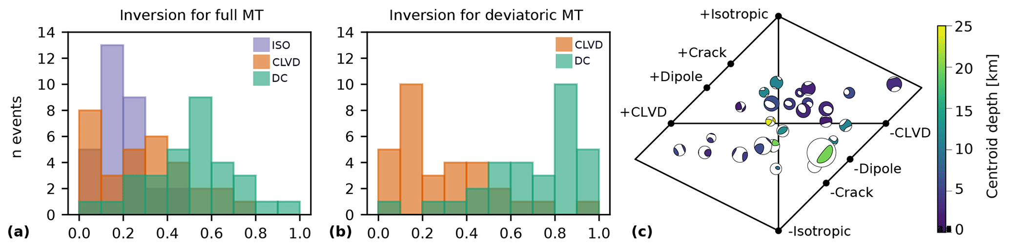
Figure 4Histograms showing the decomposition of the full (a) and deviatoric (b) MT inversion results into isotropic (ISO), compensated linear vertical dipole (CLVD) and double couple (DC). Each bar of 10 % width (x axis) indicates for how many test earthquakes (y axis) the proportion of decomposition is found. For example, an isotropic component of 10 %–20 % is found for 13 test events in the full MT inversion. (c) Hudson plot showing non-DC components of individual events. Four events with Kagan angles > 60∘ between full and deviatoric solutions were removed, since they were not well resolved. Color represents depth, and beach ball size represents magnitude.
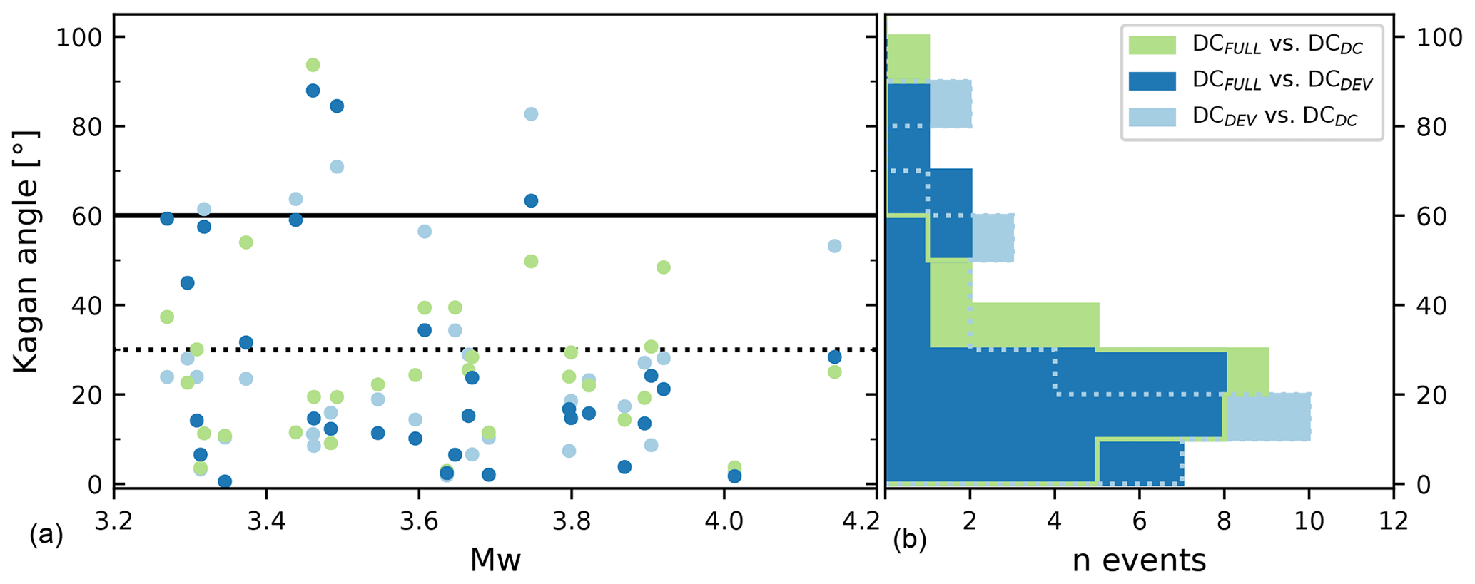
Figure 5(a) Kagan angle between DC of pure double-couple, deviatoric and full MT solutions for 30 earthquakes, Mw 3.3–4.5. The dashed and solid lines indicate Kagan angles of 30 and 60∘, respectively, indicating levels of high agreement and corresponding mechanisms. (b) Histograms showing the distribution of Kagan angles between the DC of pure DC, deviatoric, and full MT inversion solutions.
The DC component is representing the purely tectonic shear dislocation (e.g., Miller et al., 1998; Julian et al., 1998; Cesca et al., 2013); therefore, it is crucial to resolve this component unambiguously. We compare the DC component that we obtain from the decomposition of the deviatoric and the full MT with the pure DC inversion result by computing the smallest rotation angle (Kagan angle, Kagan, 1991) between them to assess the stability of the DC components (Fig. 5). Rotations below 30∘ are generally accepted as representing very similar mechanisms, while a Kagan angle ≪ 60∘ is still described as corresponding (Pondrelli et al., 2006; d'Amico et al., 2011). A total of 70 % of the earthquakes have a very stable DC, with Kagan angles below 30∘ between the three solutions. In the case of about 10 % of the events, a Kagan angle ≥ 60∘ is found. These larger deviations result predominantly from large non-DC components in the full inversion result (in >70 % of these events). In these cases, the CLVD combined with the isotropic component shows orientations similar to the DC component of the pure DC and the deviatoric inversion result. Therefore, the resulting focal sphere is similar, while the DC component deviates from the pure DC inversion result. Overall, the results of this test indicate that the DC component is in most cases very well resolved, independently of allowing for a CLVD and an isotropic component.
In the following, we present a more detailed analysis of an exemplary earthquake with a significant non-DC components: 28 May 2019, Mw 3.9, close to Lake Geneva, France (Fig. 6a). Figure 6b depicts the MT decompositions of the MTs obtained with a pure DC inversion, a deviatoric inversion, and a full MT inversion. All three inversions were performed using the same inversion setup (full waveforms and amplitude spectra; Z, R, and T components; 73 stations; 0.02–0.07 Hz). The DC component is similar for all inversion types, but the deviatoric and full inversion results indicate significant non-DC components.

Figure 6Earthquake close to Lake Geneva (France–Switzerland border region), Mw 3.9, 28 May 2019, 08:48:06 UTC. (a) Seismic network used for the MT inversions (73 broadband sensors, red triangles) and synthetic network (circle of blue dots, in 1∘ steps). (b) Decomposition of the full (purple), deviatoric (orange), and pure DC (green) MT inversion solution with the smallest misfit. (c) Hudson plots showing the ensemble of solutions for the full and the deviatoric MT inversions; colors are as in (b). Larger symbols depict the best solutions of (b). (d) For the three MT solutions (full, deviatoric and DC) synthetic data were forward-computed for the fictional network shown in (a). For each component (Z, R, T), the first row shows the maximum cross-correlation values of the three synthetic traces at each station (BP filter 0.02–0.1 Hz). The second row shows the maximum absolute amplitude at each back-azimuth, normalized over the three solutions. The dashed lines indicate the strike 1 and 2 directions of the two nodal planes of full, deviatoric, and DC solutions and their 180∘ equivalent.
To investigate whether the resolved non-DC components are unambiguous, we forward model synthetic waveforms of the three MT solutions recorded at fictional receivers in 250 km distance in azimuthal steps of 1∘ (Fig. 6a). We use a bandpass filter of 0.02–0.1 Hz, which is even wider than the frequency range used in the MT inversion (0.02–0.07 Hz) to assess the similarity of the entire modeled surface wave trains. By cross-correlating the forward modeled waveforms, we find that the full and deviatoric sources produce very similar waveforms on all seismometer components in all back-azimuthal directions (Fig. 6d). Furthermore, the maximum amplitudes between the deviatoric and full solution differ only slightly. This indicates that the non-DC component can be comparably well represented by a CLVD or by a combination of an isotropic plus a CLVD component.
A comparison of the forward modeled waveforms from a pure DC solution with a full or deviatoric solution shows very high correlations in all azimuthal directions on the T components (Fig. 6d, lower panel). Neither the CLVD nor the isotropic component is influencing the transversal Love wave. On R and Z components, the resulting waveforms show cross-correlations below 0.9 in strike-direction only (Fig. 6d, upper and middle panel). This indicates that in the case of this event, without any station covering this ray path direction, we cannot resolve the difference between a pure DC MT and a full or deviatoric one.
The true azimuthal coverage of seismic stations is much denser to the NE and E than in the strike direction (Fig. 6a). Forward modeling the waveforms of the 73 used stations results in a similar but less well-resolved pattern compared to Fig. 6d. The uneven azimuthal distribution and the lack of stations in strike directions hinders the unambiguous identification of non-DC components.
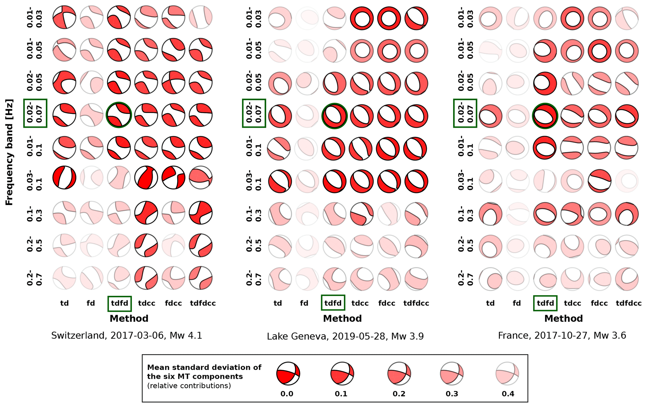
Figure 7Testing of input data types and frequency ranges for three earthquakes with magnitudes between Mw 3.6 and 4.1. Abbreviations are as follows: td is time domain full waveforms; fd is frequency domain amplitude spectra; cc is cross-correlation fitting of full waveforms; tdfd, tdcc, fdcc, and tdfdcc are combinations of these. Color intensity represents summed uncertainty of MT components. A combination of fd and td in a frequency band between 0.02–0.07 Hz yields the best results for Mw>3.3 (marked in green).
This example shows that whenever we investigate large non-DC components in a deviatoric or full MT inversion, one must assess the resolution and the validity of the results. The synthetic tests indicate that including full waveforms of body waves at higher frequencies in the inversion clearly helps to improve the resolution of non-DC components. However, due to the station spacing, the relatively high noise level, and the low resolution of crustal velocity models, we cannot use higher frequencies for most events in this study. Following our findings, we report deviatoric MT inversions in the result section and only perform inversions for the full MT in the case of large non-DC components for comparison.
2.2.2 Frequency ranges and input data type
In previous studies, dependencies of the MT inversion results on the inverted frequency band have been observed and multistep inversion workflows including several frequency bands were proposed (e.g., Barth et al., 2007). In order to find the best combination of frequency ranges and time domain or frequency domain input types for the MT inversion, we selected a subgroup of 13 earthquakes recorded by the AlpArray stations. These test events span a magnitude range of Mw 3.3 to 4.1 and are therefore considered representative. We perform MT inversions using different combinations of input data types (Figs. 7 and S1 in the Supplement): time domain full waveforms (td), frequency domain amplitude spectra (fd), cross-correlations of time domain full waveforms (cc), waveform envelopes, and combinations thereof. The input data are filtered using nine different bandpass filters with passbands between 0.01 and 0.7 Hz (Figs. 7 and S1). We compare the uncertainties of the resolved MTs in order to find the most appropriate parameter settings for our study and future MT studies in the Alps or similar settings.
In Fig. 7, we show the results for three exemplary events. The color intensity of each focal sphere represents the summed standard deviations of the six MT components derived from the ensemble of solutions of the bootstrap chains. Intense colors represent stable solutions with low uncertainties. The first event is a Mw 4.1 earthquake in Switzerland. Due to the high magnitude, the MT inversion results are stable over frequency bands ranging from 0.01–0.03 Hz up to 0.01–0.10 Hz for all input data types. The MT is not well resolved when filtering using a passband of 0.03–0.1 Hz or higher. A similar behavior is observed for the second example, a Mw 3.9 normal faulting event close to Lake Geneva. The MT is very well resolved using bandpass filters covering the intermediate passbands between 0.02 and 0.1 Hz. In contrast to the first event and corresponding to the lower magnitude, the resolution is worse when frequencies between 0.01–0.02 Hz are included, while the frequency band between 0.03–0.1 Hz still leads to satisfying results. In general, the higher the frequency band, the lower the stability of the ensemble of solutions due to the simplified 1-D velocity model, site effects, and increased noise levels.
In the case of the third example (Fig. 7), a Mw 3.6 earthquake from France, the MT solutions vary substantially. This illustrates the need for a careful selection of appropriate methods and frequency ranges and the analysis of the uncertainties of MT inversions. For both the higher-frequency ranges (from 0.03–0.1 Hz and higher) and the lowest-frequency bands (0.01–0.03 and 0.02–0.05 Hz) surface waves have insufficient SNRs. Stable results for most input types are obtained in the frequency band 0.02–0.07 Hz, in which surface waves are more distinct. A visual inspection of the recorded waveforms of various events with magnitudes of Mw 3.4–3.9 confirms that surface waves have highest SNRs for periods between 0.02 and 0.05 Hz. Extending the passband to 0.02–0.07 Hz helps to avoid mismatching monochrome phases in the inversion process.
Comparing the different input data types for all 13 test events, we find that a combination of frequency domain amplitude spectra and time domain full waveform fitting (tdfd in Fig. 7) provides more stable results than relying on time domain waveform fitting alone. The high uncertainties of the frequency domain amplitude spectra fitting alone (fd) result from the unresolved polarity. The geometry of the nodal planes can still be determined. For most events, the other combinations (tdcc, tdfccc, fdcc) provide more stable results compared to using only time domain full waveforms (td). However, compared to the tdfd combination, they do not further improve the stability of the solution.
In addition to the presented tests of input data types, we tested waveform envelopes (Fig. S1). In order to resolve the polarity of the mechanisms, the envelopes are combined with time domain full waveforms or cross-correlation fitting of waveforms at nearby stations. This is a reasonable setting for weak events, where full waveforms may be of such low amplitudes that they can only be fitted at closer stations while envelopes of more distant stations may still be of use. We find that in the case of intermediate- or large-magnitude test events (Mw≥3.6), the resulting MT is well recovered, although uncertainties are larger than with a time domain–frequency domain combination. In the case of smaller events, where time domain–frequency domain combinations might fail, the envelopes may stabilize the inversion. The applicability of the combination of envelopes and nearby time domain traces depends on the data quality of the closest stations and on the careful selection of the frequency range and the smoothing of the waveform envelopes.
Following the results of our methodological tests, we routinely use a combination of frequency domain amplitude spectra and time domain full waveform fitting in a frequency band of 0.02–0.07 Hz for earthquakes with Mw>3.5. In the case of smaller-magnitude earthquakes, we additionally perform inversions using a frequency range of 0.03–0.10 Hz. We observe that in the case of low-magnitude earthquakes the initial local magnitudes can differ significantly from our moment magnitude estimates. Furthermore, the availability of stations with a good SNR depends not only on the event magnitude but also on noise conditions and damping along the travel path. It is therefore necessary to adapt the approach to the individual earthquakes, but the two frequency ranges constitute reasonable guidelines.
2.2.3 Station coverage
The dense AASN provides an excellent azimuthal distribution of seismic stations for moderate to large earthquakes in the Alps. We take advantage of the large number of stations in the AASN to investigate how the stability of the deviatoric MT inversion is influenced by gaps in the azimuthal station distribution around an earthquake. This allows simulating uncertainties of MT solutions in the marginal areas of the AASN, but the results also apply to other locations and networks (e.g., close to subduction zones). Most generally, within the AASN larger event-station distances can be taken into account for larger magnitude earthquakes and therefore both the number of stations and the azimuthal station coverage increases. In contrast, individual malfunctioning stations may already result in large azimuthal gaps for low magnitude earthquakes located within the AASN. In theory, the DC components of a moment tensor can be resolved from a single station using 3-component data (Dufumier and Cara, 1995). However, such an analysis requires high data quality and exact knowledge about velocity structures and path effects. In practice, single-station approaches are mostly avoided as they often result in unstable solutions (Dufumier and Cara, 1995).
Figure 8 shows the fuzzy MTs (right panels) for decreasing azimuthal coverage of seismic stations (left panels) for three exemplary events. In the case of the largest event (Mw 4.1), the solution is very stable when seismic stations cover at least an azimuthal range of 90∘. In the case of an even smaller coverage, the mechanism rotates slightly depending on the azimuthal direction of the remaining stations. In the case of the Mw 3.9 event, the uncertainties of the solutions increase with decreasing station coverage. Two examples in which the inversions were done with stations covering only an azimuthal range of 45∘ show significant differences between the resulting focal mechanisms. When only considering the fuzziness of the two focal mechanism plots, both ensembles of solutions seem to be well resolved and stable. This indicates that the amount and variability of input data are not sufficient to resolve the MT unambiguously.
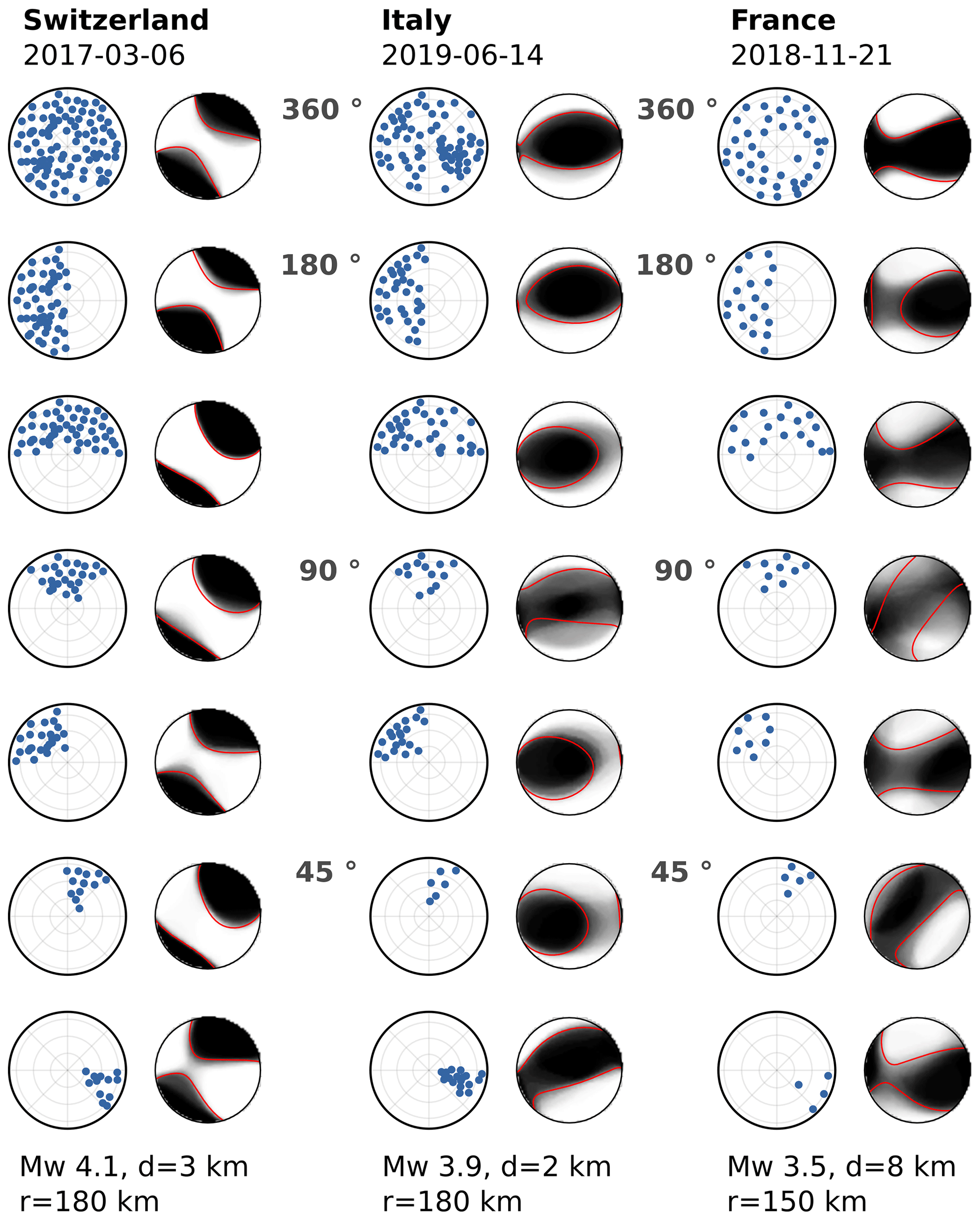
Figure 8Resolution of the deviatoric MT depending on the azimuthal station coverage for three earthquakes with magnitude Mw, centroid depth d, and event-station radius r given below each column (left, middle, and right panels). The station coverage (blue dots in the first, third, and fifth columns) decreases from top to bottom as indicated in between the event columns. The fuzzy MTs show the solution stability (Sect. 2.1 and Fig. 2). They are composed of the superimposed P radiation pattern of the ensemble of solutions from the bootstrap chains.
Furthermore, we observe a clear trend of increasing non-DC components with decreasing azimuthal coverage. We find a non-DC component below 10 % for a coverage of 180∘ but 40 % for the smallest tested coverage for the Mw 3.9 event.
For the smallest earthquake (Mw 3.5), the resulting MT solutions vary even more. In the case of the inversions with a station coverage of 90∘, the variability among the ensembles of solutions is high and depends on the location of the 90∘ quadrant covered with stations. When only considering the dominant DC components of the deviatoric moment tensors, we observe the same general correlation between coverage and resolution. It is worth noticing that even with a small number of stations covering a small azimuthal range, it is possible to resolve a MT under favorable geometrical conditions. When stations are located in strike direction and cover both tensional and compressional quadrants, they may resolve the MT correctly even when covering only 45∘ (Fig. 8, Mw 3.5 event, fifth row and last row).
We conclude that in the case of larger earthquakes with a high SNR and a sufficient number of stations at different epicentral distances even a limited azimuthal coverage does not necessarily pose a problem, but lower-magnitude earthquakes usually require a better azimuthal station coverage. In regard to a semi-automated MT inversion workflow, we implemented an optional minimum station distribution threshold. Based on our results, and since we do not assume any a priori known strike direction, we limit the inversions to earthquakes with an azimuthal coverage above 90∘ but thoroughly evaluate all results with a coverage below 180∘.
3.1 CMT solutions for the Alpine region, 2016–2019
Based on our methodological tests, we use a combination of time domain full waveforms and frequency domain amplitude spectra as input data for the centroid MT inversion for earthquakes larger than Mw 3.0. We choose a frequency range of 0.02 to 0.07 Hz for a first inversion of each event. Depending on the event magnitude, the maximum epicentral distance varies between 80 and 300 km. In the case of poor fits, we slightly increase the frequency bands (0.03–0.1 Hz for ) for smaller events and decrease it for the larger events (0.02–0.05 Hz for Mw>4.2). Deviatoric inversions were generally favored over full moment tensors since we demonstrated that the isotropic and CLVD components can often not be distinguished reliably. In addition, no volume changes are expected to accompany small earthquakes in the seismotectonic setting of the Alps. We obtained deviatoric MT solutions for 75 earthquakes occurring between January 2016 and December 2019 in the wider Alpine region for which we determine moment magnitudes between Mw 3.1 to 4.8 (Fig. 9, Table S1 in the Supplement). While we were able to compute stable MTs for most Alpine earthquakes from regional catalogs with local magnitudes larger Ml 3.3, we resolved only 13 MTs for earthquakes with local magnitudes between Ml 3.1 and 3.3, corresponding to one-third of the events in this magnitude range compared to the GEOFON catalog. Low SNR in the tested frequency bands covering frequencies between 0.02 and 0.5 Hz and fewer available stations hindered successful inversions for the other small earthquakes. Furthermore, we realized that a station spacing of about 60 km is not sufficient for small earthquakes (Mw<3.3) in case a part of the data is rejected due to quality issues.
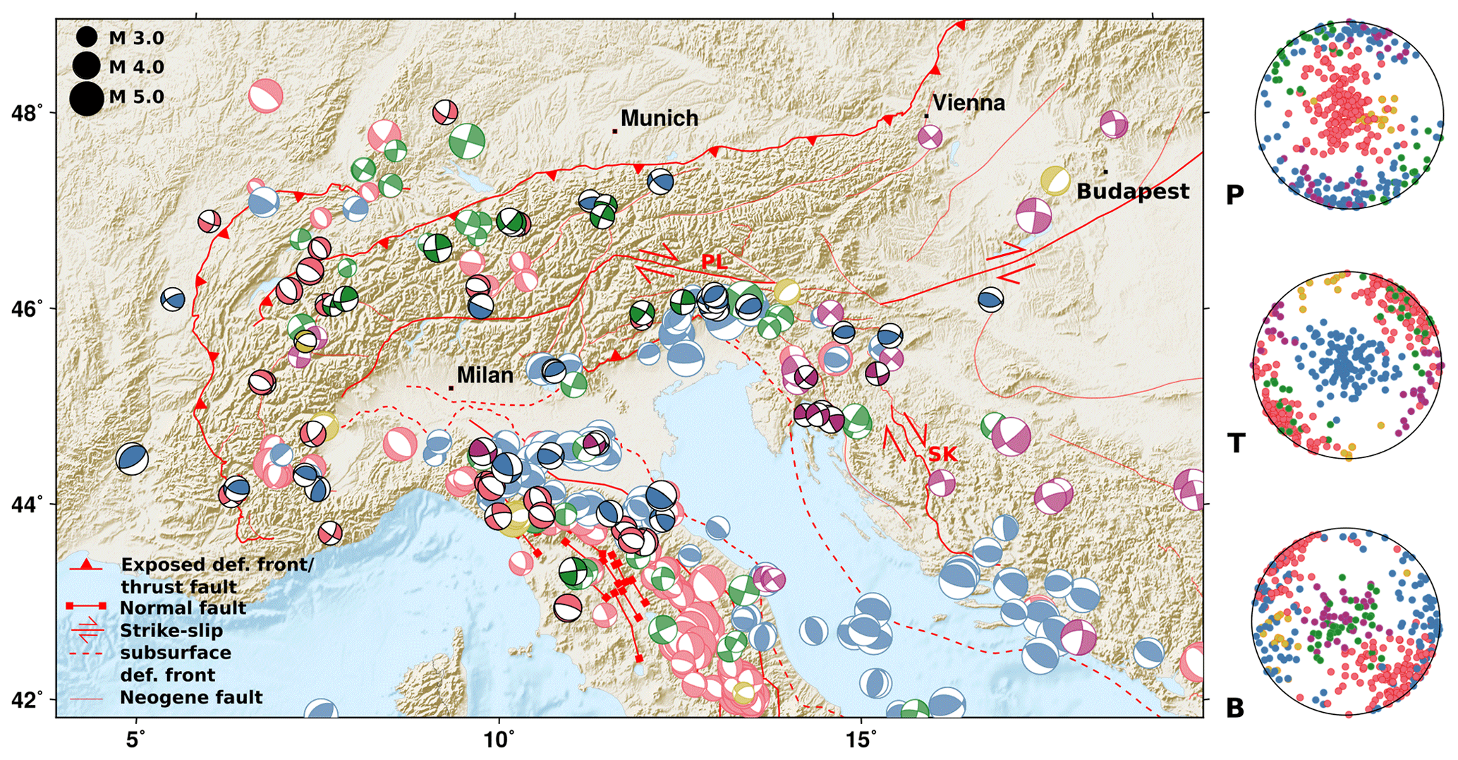
Figure 9Moment tensor inversion results from January 2016 to December 2019 (focal spheres with black lines) along with MTs from 1983–2015 from bulletins of GCMT, GEOFON, INGV, SED, EM-RCMT, and ARSO (lighter colors). Similar colors represent clusters of comparable mechanisms obtained from a clustering approach based on the smallest rotation between the mechanisms (see text). Red and orange colors correspond to dominant normal faulting mechanisms in a cluster. Thrust faulting is indicated in blue, and strike-slip faulting earthquakes are colored in green and purple. Exposed and subsurface faults are simplified from Schmid et al. (2004, 2008), Handy et al. (2010, 2015), and Patacca et al. (2008). “PL” marks the Periadriatic line, and SK marks the Split–Karlovac Fault. (right) Pressure (P), tension (T), and null (B) axis of all focal mechanisms. Topographic data from SRTM-3 (Farr et al., 2007) and ETOPO1 (Amante and Eakins, 2009) datasets.
For about 40 % of our own MT solutions for 2016 to 2019, no MT solutions were available from regional observatories (INGV, GEOFON, EM-RCMT, SISMOAZUR, SED, ARSO). For the other earthquakes, we obtain similar MT solutions, with a median deviation Kagan angle of 21∘ (mean of 24∘). For the largest events, the deviation is 15∘. In the following, we jointly analyze our results with approximately 350 moment tensors of earthquakes that occurred before 2016, as reported by GCMT, GEOFON, INGV, EM-RCMT, SED, and ARSO (Fig. 9). Whenever more than one MT solution is available from the different bulletins, we prioritize local institutes (INGV for Italian earthquakes, SED for earthquakes in Switzerland, ARSO for Slovenia), unless they indicate high uncertainties. Furthermore, EM-RCMT with great experience for the Mediterranean and surrounding areas is favored over GEOFON solutions and over GCMT.
We used a clustering algorithm (Cesca, 2020) based on the Kagan angles between all focal mechanisms obtained in this study and reported in the catalogs to define classes of similar mechanisms (Fig. 9). The clustering tool uses the DBSCAN clustering algorithm (Ester et al., 1996), which relies on two parameters, the maximum acceptable similarity distance (eps) between two events, here eps = 0.14, and the minimum number of neighboring items (nmin), here nmin = 6. We choose a rather large eps value to emphasize patterns of general similarity between mechanisms. In a second step, we assign all remaining earthquakes to the cluster to which they have the smallest rotation angle.
Within the Alps, we observe four dominant groups of focal mechanisms (Fig. 9). Roughly E–W-striking thrust faulting is observed in the eastern Southern Alps (northern Italy) and at the central southern margin of the mountain range (blue focal spheres). A group of similar strike-slip-faulting earthquakes are aligned parallel to the northern deformation front of the Alps (green focal spheres, Fig. 9). A second group of strike-slip mechanisms is situated in the transition of the Alps to the Dinarides and in the northern Dinarides (purple and green focal spheres). NW–SE-striking normal faulting events are found in the NW Alps (red focal spheres), while mechanisms are more heterogeneous in the SW Alps.
3.2 Distribution of centroid depths
The resolved centroid depths within the Alps range from about 2 to 15 km, pointing to a shallow seismic activity within the mountain range. A total of 80 % of the studied events have depths shallower than 10 km. A comparison of our inverted centroid depths to the depths published in the event catalogs is limited for two reasons. First, the event depths were fixed in some of the published moment tensor inversion results, and second the depth estimates differ significantly among the different catalogs. We find a good correspondence with less than 3 km difference for >60 % of the events to at least one of the published solutions. For another 26 %, we report differences between 3 and 5 km.
In Fig. 10, we display the depth distribution of mechanisms depicted in Fig. 9 sorted by faulting type. In the left panels, the focal mechanisms derived from the aforementioned bulletins are shown, while our own centroid solutions are provided in the right panels. While the depth in the catalogs may be partly fixed during the inversion, the centroid depth is determined during the MT inversion in our approach. Uncertainties of our solutions are mostly in the range of 1 to 3 km. Many events within the Alpine mountain range are shallower than 10 km (Fig. 10d–f). While we obtained depths below 5 km for all normal faulting events in the NW Alps, depths of up to 15 km are observed for thrust-faulting events occurring between 2016 and 2019 in the eastern Southern Alps.
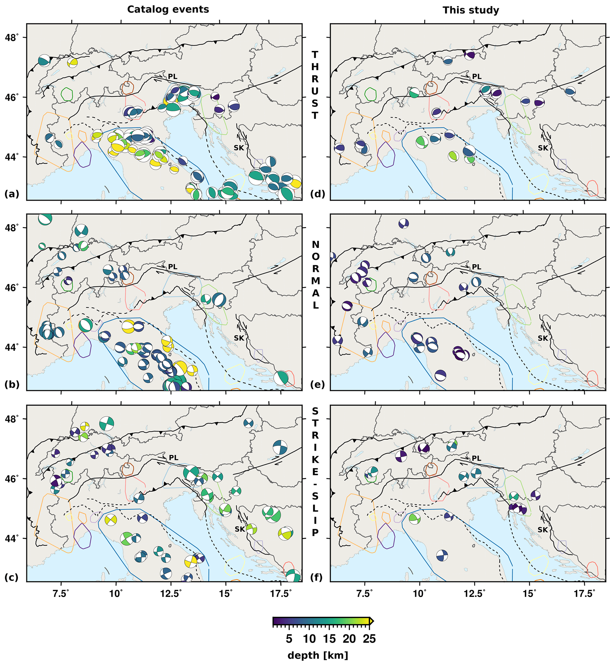
Figure 10(a–c) Catalog depths of earthquakes shown in Fig. 9. Depths may be fixed in some catalogs. (d, e) Centroid depths of MT solutions in this study. Earthquakes are sorted according to their mechanisms: (a, d) thrust-faulting events, (b, e) normal faulting events, and (c, f) strike-slip events. Exposed and subsurface faults (solid and dashed lines) are simplified from Schmid et al. (2004, 2008), Handy et al. (2010, 2015), and Patacca et al. (2008). PL marks the Periadriatic line, and SK marks the Split–Karlovac Fault. The outlines of spatial clusters of increased seismic activity from Fig. 12a are indicated for orientation.
Centroid depths in the Apennines can be significantly larger. Thrust and normal faulting events are roughly separated into two NW–SE-running bands, with more thrust events in the NE and more normal faulting events in the SW part. Normal faulting and strike-slip events occur predominantly at shallower depths (<20 km) than the thrust-faulting events with depths of often 30–50 km.
4.1 Dominant mechanisms and the regional stress regime
The distribution of our mechanisms coincide well with long-term seismological and tectonic observations. The moment tensor solutions obtained from small to moderate earthquakes during 4 years with an enhanced station density in the course of the AlpArray project allows for identifying multiple seismotectonic domains. The faulting styles of these domains are in agreement with those derived from longer-term moment tensor catalogs (Fig. 9). Furthermore, new solutions for regions of sparse seismicity like the northern Central Alps provide new insights into recent activity. Thrust faulting related to the N–S compression between the European plate and the Adriatic plate is mainly observed in the eastern Southern Alps, strike-slip faulting is observed in the northern Dinarides and along the northern Alps and normal faulting is observed in the NW Alps (Fig. 9).
The orientations of P and T axes of the moment tensor solutions across the Alps provide information on local deformation regimes. Their distribution across the mountain belt points out both local and regional heterogeneities (Fig. 11). In addition to the direct interpretation of P and T axes, we apply a stress inversion approach based on the minimization of the seismic energy released on unfavorably oriented faults (Cesca et al., 2016) in volumes of comparably high seismic activity (Fig. S2). Stress inversion results provide the orientations of the most compressive (σ1), the intermediate (σ2), the least compressive principle stresses (σ3), and the relative stress magnitude . A homogeneous stress field is assumed within the selected rock volume and time period for each subregion.
In the following, we describe the patterns of P and T axes, as well as the local stress regimes in the different seismotectonic domains, which were inferred from the moment tensor solutions. In doing so, we first concentrate on the typical N–S compressional regime in the central to eastern Southern Alps (Region 2 and 3 in Fig. 1), before we focus on the transition to the strike-slip regime in the northern Dinarides (Region 4 in Fig. 1). Subsequently, the deformation regime in the Western Alps (Region 1 in Fig. 1) is discussed. Additionally, we discuss the findings for the neighboring northern Apennine mountain range (Region 5 in Fig. 1).
At the southern margin of the central Southern Alps, we observe predominantly thrust mechanisms with NNW–SSE-to-NW–SE-oriented P axes in the central Alps, close to Lake Garda, to NNE–SSW-oriented P axes further east (Fig. 11a, features d and e). Our stress inversion results confirm dominating compression from the central to eastern Southern Alps with sub-horizontal σ1 orientation (Fig. S2), which is in agreement with the stress map of the Mediterranean and Central Europe (Heidbach et al., 2016). Seismic activity at thrust faults originating from the N–S convergence of the Adriatic and Eurasian plates in the Southern Alps are well known and have been described by various studies (e.g., Pondrelli et al., 2006; Anselmi et al., 2011; Poli and Zanferrari, 2018). According to Cheloni et al. (2014), the SE Alpine thrust front absorbs about 70 % of the convergence between the continental plates. In the transition from the Southern Alps to the northern Dinarides a rotation of the P axes from NW–SE to NNE–SSW is observed (Fig. 11a, features a–c). Despite increased uncertainties due to the relatively low number of available MT solutions, we observe a similar rotation of σ1. Although less distinct, this rotation can also be seen when looking at the stress direction obtained from thrust MTs in Heidbach et al. (2016). The changes in the orientation of the thrust mechanisms may be attributed to the bending of the southern thrust front of the Alps and to the transition to the strike-slip fault systems in the Dinarides.
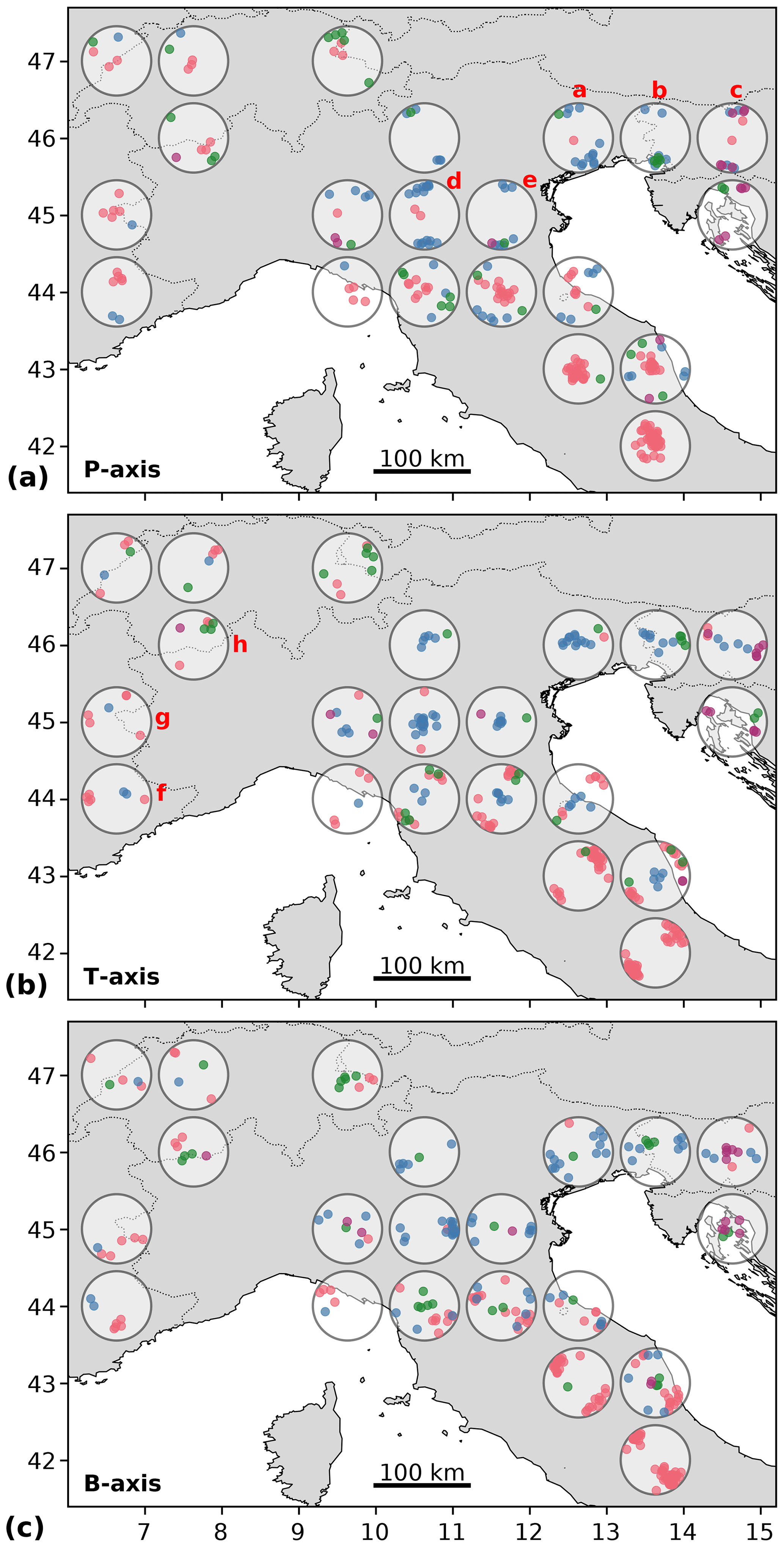
Figure 11Regional distribution of (a) P, (b) T, and (c) B axes of focal mechanisms presented in Fig. 9. Colors correspond to mechanism classes as shown in Fig. 9. Only areas with more than five events in a latitude–longitude grid of are shown. Areas a to h mark features that are discussed in the text.
The transition from dominant thrust faulting close to Friuli to the strike-slip events to the east and in the northern Dinarides was also described by Pondrelli et al. (2006) and is mapped by the change from a sub-vertical to an almost horizontal σ3 direction (Fig. S2). Moulin et al. (2016) describe right‐lateral motion (3.8±0.6 mm yr−1) on three main Dinaric faults and suggest that the system of NW–SE-oriented right-lateral strike-slip faults might be the northeastern boundary of the Adriatic microplate.
The W Alps show more heterogeneous faulting compared to the Southern Alps and the northern Dinarides. We obtained four new MT solutions indicating NW–SE-striking normal faulting east of Lake Geneva in the NW Alps, in agreement with the orientation of T axis at a high angle to the bending of the orogen described by Delacou et al. (2004). Our MT solutions and the catalog solutions show normal faulting, thrust faulting, and some oblique strike-slip faulting events in the W to SW Alps (Region 1 on Fig. 1). Despite the small number of moment tensors, we can also infer a rotation of the T axes in the southwestern Alps. In contrast to the northwestern Alps, where the tensional axis points at an extension along the mountain belt, the T axes of the focal mechanisms are oriented roughly perpendicular to the Alpine arc (Fig. 11b, features f and g). The stress inversion results indicate an extensional regime in the Western Alps with a sub-vertical σ1 orientation. However, across the large region the uncertainties of the stress inversion are relatively high. This is in agreement with the co-existing thrust faulting, normal faulting, and strike-slip faulting also shown by Delacou et al. (2004) and Heidbach et al. (2016).
Along the Apennines, thrust faulting is dominant at the northern arc, while normal faulting earthquakes are dominant southwest of the ridge of the Apennines. The NW–SE orientations of the T axes of the normal faulting events are perpendicular to the elongation of the mountain belt as also described by Pondrelli et al. (2006). The vertical σ1 direction and the NE–SW-oriented, horizontal σ3 direction confirm an extensional stress regime (Fig. S2). In contrast, a compressional regime is observed along the NE arc of the Apennines with P axes of the thrust-faulting events oriented NW–SE to NE–SW (Fig. 11).
4.2 CMT solutions in the seismotectonic context
Since only a few focal mechanisms are available for large parts of the Alps, we additionally take into account recent seismicity (Fig. 12a, c and d), historical large earthquakes (Fig. 12b), and GNSS data (Fig. 12e and f) to analyze our results in the seismotectonic context and draw a more detailed picture of the seismic and tectonic activity in the study area. To emphasize areas of significant seismic activity (Fig. 12a), we cluster the earthquakes in the seismicity catalogs by INGV, GEOFON, and GCMT according to their epicentral locations using the DBSCAN clustering algorithm (Ester et al., 1996) implemented in the Python package scikit-learn (Pedregosa et al., 2011). The merged catalog comprises more than 50 000 earthquakes with Ml>2.0 (1983–2017). The recent seismic activity can be traced back to historical times. Figure 12b shows historical earthquakes from the European Archive of Historical Earthquake Data 1000-1899 (AHEAD; Locati et al., 2014; Rovida and Locati, 2015) based on the SHARE European Earthquake Catalogue (SHEEC; Stucchi et al., 2013) and the ISC-GEM catalog (Storchak et al., 2013, 2015; Bondár et al., 2015; Di Giacomo et al., 2015, 2018) with Mw>5.5.
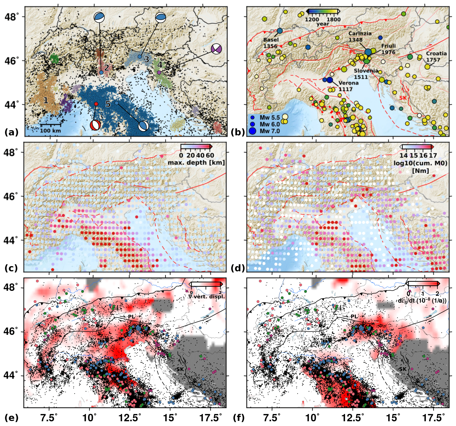
Figure 12Characteristics of recent and historical seismicity and strain from GNSS data. (a) Seismic activity between 1978 and 2017; Ml>2.0; from GEOFON, INGV, and GCMT catalogs; and colored according to epicentral clusters of seismicity. Representative MTs from Fig. 9. Numbers refer to regions (1) W Alps, (2) Lake Garda, (3) eastern S Alps, (4) N Dinarides, and (5) Apennines. (b) Historical earthquakes with Mw>5.5 from the European Archive of Historical Earthquake Data 1000–1899 (AHEAD) (Locati et al., 2014; Rovida and Locati, 2015; Stucchi et al., 2013) and ISC-GEM catalog (1906–2016) (Storchak et al., 2013, 2015; Bondár et al., 2015; Di Giacomo et al., 2015, 2018). (c, d) Maximum event depth and the cumulative seismic moment on a grid with a spacing of latitude and longitude. (e, f) Absolute value of the spatial gradient of the relative uplift rate as a proxy for vertical strain rates and observed GNSS shear strain rate (second invariant of strain tensor); both are obtained from GNSS data of the EUREF WG on European Dense Velocities (Brockmann et al., 2019). Black dots indicate seismicity, Ml>2.0. Events with MT solutions are color-coded as in Fig. 9. Exposed and subsurface faults (solid and dashed lines) are simplified from Schmid et al. (2004, 2008), Handy et al. (2010, 2015), and Patacca et al. (2008). PL marks the Periadriatic line, and SK marks the Split–Karlovac Fault. Topographic data are from the SRTM-3 (Farr et al., 2007) and ETOPO1 (Amante and Eakins, 2009) datasets.
In general, the seismicity along the southern margin of the Alpine mountains is higher than along its northern counterpart. Apart from the large cluster of seismicity in the Apennines, we identify five dominant clusters and several smaller ones mainly located at the margins of the Alps (Fig. 12a). The largest seismicity clusters correspond to the numbered regions shown in Fig. 1. To avoid confusion with the mechanism-based clustering we here continue writing region (R) when referring to these clusters of epicenters. We focus on the analysis of the largest clusters, for which we were able to obtain multiple moment tensor solutions between 2016 and 2019. Following the Alpine arc from west to east, the first cluster is located in the Western Alps at the French–Italian border (R1 in Figs. 12a and 1), and two smaller clusters are found in the region around Lake Garda in the central Southern Alps (R2) and north of it. Two more clusters of high seismicity are situated in the eastern Southern Alps in the border region between Italy (Friuli) and Slovenia (R3), and in the northern Dinarides (R4). Figure 12a indicates dominant faulting styles for each cluster, namely thrust faulting for regions 2 and 3 around Lake Garda and in the eastern Southern Alps and strike-slip faulting in the northern Dinarides (R4). In the epicentral cluster of the Apennines (R5), two representative mechanisms reflect the separation of dominant normal and thrust-faulting earthquakes SW and NE of the ridge, respectively. Due to the heterogeneous faulting in the Western Alps, we assign no representative mechanism.
The cluster of high seismicity in the eastern Southern Alps (Fig. 12a) is located close to the epicenter of the 1976 Friuli earthquake (Mb 6.0; Pondrelli et al., 2001). The observed E–W-striking thrust events map the regional dominant stress field (Fig. 9), evolving from the underthrusting of the Friuli Plain beneath the Alps (e.g., Cipar, 1980). Focal mechanism solutions of the 1976 mainshock and aftershocks show similar thrust mechanisms, partly with a small strike-slip component, and are associated with the complex Periadriatic overthrust system (e.g., Cipar, 1980; Bressan et al., 1998; Pondrelli et al., 2001, 2006; Poli and Zanferrari, 2018; Slejko, 2018). Only a few tenths of kilometers to the west of the Friuli area we observe strike-slip faulting (Fig. 9). Anselmi et al. (2011) report the occurrence of both thrust and strike-slip faulting for this area, mostly in agreement with an E–W to ENE–WSW minimum horizontal stress reported by Montone et al. (2004). Large historical events are reported along the southern margin of the Alps between Lake Garda (R2), the eastern Southern Alps (R3), and the transition to the northern Dinarides (R4) (Verona 1117, Slovenia 1511, and Carinthia 1348, all Mw≥6.7). Similar high-seismicity and cumulative seismic moments during the last decades (Fig. 12d) are observed here. Within the seismicity cluster close to Lake Garda, Italy, the observed thrust mechanisms are typical for earthquakes located in the Giudicarie region close to the Ballino–Garda fault that runs through Lake Garda (Viganò et al., 2008).
Less frequent large historical earthquakes with magnitude estimates between Mw 5 and 6 are reported in the Western Alps and the Dinarides (R2 and 4). Within the last decades, earthquakes with are observed across a wider part of the Western and Southern Alps, but magnitudes rarely exceed Ml 3.5 in large areas of the Central to NE Alps. The Eastern Alps north of the Periadriatic line and the area between the seismically active regions in the Western Alps and the Central Alps have particularly low seismicity rates (Fig. 12a). While at least three large earthquakes occurred in the eastern part of Switzerland in historical times, seismicity in this region appears to be relatively low in recent years (Fig. 12a and b).
The observed depth ranges of our MT solutions (Fig. 10) are in accordance with the maximum depths in the long-term seismic catalogs of GCMT, INGV and GEOFON, including >50 000 earthquakes with Ml>2.0 (Fig. 12c). While the Moho depth increases gradually from less than 30 km at the northern margin of the Alps to above 50 km in the central part of the orogen (Spada et al., 2013), we do not observe any gradual change in the event depth. The catalogs and our own centroid depths show that seismicity is shallow across most of the Alps with rare deeper events (<30 km) at the southern margin, where the Moho is at about 40 km depth (Spada et al., 2013). These few deeper events are located above the Moho. Maximum depths of above 60 km are observed in the Apennines.
The joined interpretation of seismicity, GNSS data, and MT solutions shows how the overall spatial distribution of faulting styles in the study area can be interpreted in the regional tectonic regime. Figure 12e and f present the spatial gradient of the uplift rates and the horizontal strain rates, computed from the GNSS data of the EUREF WG on European Dense Velocities (http://pnac.swisstopo.admin.ch/divers/dens_vel/index.html, last access: December 2020, Brockmann et al., 2019). Please refer to the Supplement for additional methodological information. Following Keiding et al. (2015), we use the spatial derivative of the uplift rate as a proxy of vertical strain rates (Fig. 12e).
Within the Alpine mountain range, the GNSS data show a consistent uplift relative to the surrounding areas (Fig. S3). Figure 12e and f emphasize the relation between recent seismic activity and both high spatial gradients of the uplift rate (Fig. 12e) and the shear strain rate (Fig. 12f) across large parts of the study area. The largest gradients of the uplift rate, high shear strain rates, and highest seismicity rates are observed in the eastern Southern Alps (R3 in Fig. 12a) and in the Apennines (R5 in Fig. 12a). The distribution of the cumulative seismic moment (Fig. 12d) agrees particularly well with the distribution of shear strain rates (Fig. 12f). We observe typically E–W-striking thrust faulting in the eastern Southern Alps, as also described in many previous studies (e.g., Pondrelli et al., 2006; Poli and Zanferrari, 2018). High horizontal velocities point to the shortening and crustal thickening in the eastern Southern and Eastern Alps due to the convergence of Adriatic and European plate (Fig. S3), in accordance with Serpelloni et al. (2016) and Sternai et al. (2019). Southeast of this area, at the transition to the northern Dinarides (Regions 3–4), the uplift gradients are low, while increased shear strain rates agree with our dominant strike-slip mechanisms (see also Serpelloni et al., 2016) and right-lateral motion on the Dinaric strike-slip faults (Moulin et al., 2016).
While there is no significant shear strain in the Western and Central Alps, we depict two subparallel bands of moderate spatial gradients of the uplift rate running roughly along the northern and the southern margin of the Alps. These two bands result from the overall relative uplift of the Alps and also have higher seismicity rates compared to the central Alpine belt. In the SW Alps, the largest events cluster in the transition area between relative uplift and subsidence, indicated by the band of increased spatial gradient of the uplift in Fig. 12e. Normal faulting events are dominant. Intraplate shear strain rates are relatively low in the entire Western and Central Alps.
The Adriatic plate, which is the upper plate in the Alpine subduction zone, rotates counterclockwise relative to Europe around an Euler pole located in the western Po plain or Western Alps (D'Agostino et al., 2008; Weber et al., 2010; Le Breton et al., 2017). The rotation results in varying convergence rates across the Alps. Le Breton et al. (2017, 2021) infer a rotation of about 5.25∘ during the last 20 Myr resulting in convergence rates ranging from 5.5 mm yr−1 in the NW Adria (Western Alps) to 7.5 mm yr−1 in the NE Adria (eastern Southern Alps) (Fig. 1). In comparison, kinematic reconstructions of Van Hinsbergen et al. (2020) involve less convergence but a higher rotation of Adria relative to Europe (10∘), leading to 2.5 mm yr−1 convergence in the NW Adria to 6.25 mm yr−1 in the NE Adria. Recent GPS data indicate little to no horizontal movement in the Western Alps but more than 2 mm yr−1 NNW-ward movement of Adria in the eastern Southern Alps (see Fig. S3), which is in agreement with increased seismicity rates. The Western Alps are closer to the location of the Euler pole of the rotation of the Adriatic plate, and therefore convergence rates are lower. Recent GPS measurements and the computed horizontal strain rates even indicate the absence of convergence (D'Agostino et al., 2008, and Fig. S3). Therefore, the uplift pattern of the Western and Central Alps (Figs. 12e and S3) and the seismicity clusters in the W Alps need to be attributed to other mechanisms. Sternai et al. (2019) propose that isostatic adjustment to deglaciation and erosion and mantle-related processes such as slab detachment or asthenospheric upwelling may jointly explain the observed uplift pattern. The assumption of a stress or strain field that is not dominantly effected by the convergence of Europe and Africa was also proposed by Delacou et al. (2004) based on focal mechanisms and stress inversion in the Western Alps. Our moment tensor solutions indicating normal and strike-slip faulting, as well as the P and T axes, match these observations from GNSS data.
The seismic activity along the northern margin of the Alps is in agreement with the increased gradient of uplift in this area. However, the occurrence of strike-slip faulting earthquakes described in this study can hardly be explained by vertical strain, especially on favorably oriented faults. However, pre-existing faults may be unfavorably oriented, the stress field may be heterogeneous and local anomalies may not be resolved by the sparse GNSS network. Rather low seismicity is further observed in the eastern Po plain, where high spatial gradients of the uplift rate are observed. The high absolute gradient here can be attributed to the relative subsidence of the sediments in the Po plain (see Fig. S3) (Carminati and Martinelli, 2002) but not to a tectonic uplift which would likely be accompanied by seismic activity.
Centroid moment tensor inversion provides insight into faulting mechanisms of earthquakes and related tectonic processes. In this study, we used the AlpArray seismic network to analyze the mechanisms of earthquakes occurring from 2016 to end of 2019. Thanks to the flexible inversion tool Grond, we were able to test different inversion setups in order to derive guidelines for MT inversions in complex tectonic settings such as the Alps. These guidelines and the proposed tests can, on the one hand, facilitate future studies of faulting mechanisms in the Alps and, on the other hand, help to derive workflows to obtain reliable moment tensors in other dense networks or complex study regions. We evaluated the results with respect to their uncertainties and parameter trade-offs. For subsets of events, we tested various frequency bands, distance ranges, and different input data types comprising time domain full waveforms, frequency domain amplitude spectra, time domain cross-correlation fitting, waveform envelopes and combinations of these. In the case of our study area, for most earthquakes with magnitudes larger Mw 3.3, we find that a combination of time domain full waveforms and frequency domain amplitude spectra in a frequency band of 0.02–0.07 Hz is most suitable. The dense deployment of the AASN is ideal to study the effect of (manually introduced) azimuthal gaps. While a higher azimuthal station coverage is favorable in general, we find that a small number of stations with little azimuthal coverage may be sufficient depending on the location of the stations with respect to the strike direction of the fault. Performing CMT inversions constraining the solutions to a pure double-couple MT, a deviatoric MT, or a full MT, indicates that for the specific Alpine context with a dense network DC components are reliably resolved independent of the applied constraint. While allowing for non-DC components reduces the overall misfit, the CLVD and the isotropic components cannot be distinguished unambiguously. We propose performing similar tests prior to MT inversions for other study areas, when earthquake magnitudes are small, the crustal structure is complex, the number of stations is limited, or other factors might hinder straightforward inversions.
Relying on the results of the methodological tests, we performed deviatoric MT inversions for events with Mw≥3.1. We present 75 solutions with reasonably low uncertainties occurring between 2016 and 2019. With four years of acquisition of small to moderate earthquakes in the course of the AlpArray project, we are able to identify seismotectonic domains that are representative in faulting styles of those derived from long-term seismic observations. We compare the derived MT solutions to historical earthquakes, recent seismicity, published focal mechanisms, and GNSS deformation data. Our moment tensor results indicate that while the Alps represent a rather heterogeneous study area, the region is characterized by compartments of different tectonic movement in close proximity. Typical ENE–WSW-to-E–W-striking thrust faulting is observed in the Friuli area in the eastern Southern Alps related to the N–S convergence of the Eurasian and Adriatic plate (Pondrelli et al., 2006; Poli and Zanferrari, 2018) and counterclockwise rotation of Adria relative to Europe (e.g., D'Agostino et al., 2008; Le Breton et al., 2017). Strike-slip faulting with similarly oriented P axes is observed parallel to the northern margin of the Central Alps and in the northern Dinarides, which is in agreement with right-lateral strike-slip faults and high shear strain rates. In contrast, NW–SE-striking normal faulting events with NE–SW-oriented T axes are observed in the NW Alps. Faulting styles in the SW Alps are more heterogeneous, with a majority of events related to an extensional stress regime. Simultaneous observations of low horizontal strain rates and normal faulting earthquakes are in agreement with studies proposing that relatively high uplift rates in the Western Alps are attributed to processes other than the Europe–Adria convergence. Based on a clustering of epicenters, we identify five main seismically active regions, namely the Western Alps, the region around Lake Garda, the eastern Southern Alps, the northern Dinarides, and the Apennines. Areas of high seismicity are mostly located in the proximity of the southern margin of the Alps, where significant vertical or horizontal strain rates are reported. Maximum observed magnitudes coincide with regions of increased seismicity and significant historical earthquakes but rarely exceed Mw 5.0. In contrast, seismicity is particularly low in the Eastern Alps and in parts of the Central Alps. The depths inferred from our moment tensor inversions and the depths in seismic catalogs indicate that the seismic activity in the Alpine mountain ranges is predominantly shallow with only few events in depth greater than 15 km in the eastern Southern Alps. Significantly deeper earthquakes are observed in the Apennines.
The moment tensor inversions were performed using the free and open-source inversion tool Grond (Heimann et al., 2018). Figures were plotted using pyrocko (Heimann et al., 2019) and GMT (Wessel et al., 2013).
The topographic data for the maps were taken from the SRTM-3 (Farr et al., 2007) and ETOPO1 (Amante and Eakins, 2009) (NOAA National Geophysical Data Center 2009: ETOPO1 1 Arc-Minute Global Relief Model. NOAA National Centers for Environmental Information. Last access: December 2020).
Seismic catalogs are from the following sources: earthquake information and focal mechanisms are provided by the below-mentioned institutes. Swiss Seismological Service (SED) (Deichmann et al., 2004, 2006, 2008, 2009, 2010, 2011, 2012; Baer et al., 2005, 2007; Diehl et al., 2013, 2014, 2015, 2018; Diehl, 2020);
Slovenian Environment Agency (ARSO) (Ministrstvo za okolje in prostor Agencija RS za okolje, 2018, 2019, 2020);
INGV (Italy) (Scognamiglio et al., 2006), http://terremoti.ingv.it/en (last access: December 2020);
GEOFON (Germany) event locations were obtained from the GEOFON program of the GFZ German Research Center for Geosciences using data from the GEVN partner networks: https://geofon.gfz-potsdam.de/eqinfo/list.php (last access: December 2020);
EM-RCMT (European-Mediterranean Regional Centroid-Moment Tensors) http://rcmt2.bo.ingv.it/ (last access: December 2020), (Pondrelli, 2002);
SISMOAZUR (France) http://sismoazur.oca.eu/focal_mechanism_emsc (last access: December 2020) provide MTs obtained using FMNEAR (Delouis, 2014);
GCMT (Lamont-Doherty Earth Observatory of Columbia University, USA) https://www.globalcmt.org/ (last access: December 2020) (Dziewonski et al., 1981; Ekström et al., 2012).
Permanent seismic networks are as follows. The permanent stations of the AlpArray are part of existing European regional networks (RD – RESIF, 2018, GU – University Of Genova, 1967, CZ – Institute Of Geophysics, 1973, ST – Geological Survey – Provincia Autonoma Di Trento, 1981, G – Institut De Physique Du Globe De Paris (IPGP) and Ecole Et Observatoire Des Sciences De La Terre De Strasbourg (EOST), 1982, CH – Swiss Seismological Service, 1983, OE – ZAMG, 1987, MN – MedNet Project Partner Institutions, 1990, HU – Kövesligethy Radó Seismological Observatory, 1992, GE – GEOFON Data Centre, 1993, RF – University Of Trieste, 1993, FR – RESIF, 1995, IV – INGV Seismological Data Centre, 2006, BW – Department Of Earth And Environmental Sciences, Geophysical Observatory, University Of Munchen, 2001, SX – Leipzig University, 2001, NI – OGS and University Of Trieste, 2002, TH – Jena, 2009, OX – OGS, 2016).
The supplement related to this article is available online at: https://doi.org/10.5194/se-12-1233-2021-supplement.
The complete member list of the AlpArray Working Group can be found at http://www.alparray.ethz.ch and the complete list of the Swath-D Working Group can be found at https://doi.org/10.14470/MF7562601148.
GMP, SC, and TD conceptualized the study. GMP performed the moment tensor inversions, conceptualized and developed the methodological tests, prepared the figures, and wrote the original draft of the manuscript. SC, TD, JK, and TP developed the general project idea and acquired the funding. SC, SH, DK, and TD supervised the study. SH developed the moment tensor inversion and the software tools used in this study (Heimann et al., 2018, 2019). SH, SC, TD, and PN contributed to methodological developments. SH and PN helped to visualize the results. TD and TP performed stress field inversions. GMP, SC, and TD validated the results. The AlpArray Working Group provided access to the seismic data of the temporary network and additional background information. All co-authors reviewed and edited the manuscript.
The authors declare that they have no conflict of interest.
This article is part of the special issue “New insights into the tectonic evolution of the Alps and the adjacent orogens”. It is not associated with a conference.
We like to thank the three anonymous reviewers for constructive comments that helped to improve the manuscript. Eline Le Breton is thanked for providing helpful information for the geological and tectonic background. Peter Niemz is currently funded by the BMBF (German Federal Ministry of Education and Research) project SECURE (grant agreement no. 03G0872A).
This research has been supported by the German Science Foundation DFG From Top to Bottom – Seismicity, Motion Patterns and Stress Distribution in the Alpine Crust (project number 362440331), a subproject of “SPP 2017: Mountain Building Processes in 4D” (project number 313806092).
The article processing charges for this open-access publication were covered by the Helmholtz Centre Potsdam – GFZ German Research Centre for Geosciences.
This paper was edited by Emanuel Kästle and reviewed by three anonymous referees.
AlpArray Seismic Network: AlpArray Seismic Network (AASN) temporary component, Other/Seismic Network, AlpArray Working Group, https://doi.org/10.12686/alparray/z3_2015, 2015. a
Amante, C. and Eakins, B.: ETOPO1 1 Arc-Minute Global Relief Model: Procedures, Data Sources and Analysis, NOAA Technical Memorandum NESDIS NGDC-24, National Geophysical Data Center, NOAA, https://doi.org/10.7289/V5C8276M, 2009. a, b, c, d
Anselmi, M., Govoni, A., De Gori, P., and Chiarabba, C.: Seismicity and velocity structures along the south-Alpine thrust front of the Venetian Alps (NE-Italy), Tectonophysics, 513, 37–48, 2011. a, b, c
Baer, M., Deichmann, N., Braunmiller, J., Husen, S., Fäh, D., Giardini, D., Kästli, P., KRadolfer, U., and Wiemer, S.: Earthquakes in Switzerland and surrounding regions during 2004, Ecl. Geolog. Helvet., 98, 407–418, 2005. a
Baer, M., Deichmann, N., Braunmiller, J., Clinton, J., Husen, S., Fäh, D., Giardini, D., Kästli, P., Kradolfer, U., and Wiemer, S.: Earthquakes in Switzerland and surrounding regions during 2006, Swiss J. Geosci., 100, 517–528, 2007. a
Barth, A., Wenzel, F., and Giardini, D.: Frequency sensitive moment tensor inversion for light to moderate magnitude earthquakes in eastern Africa, Geophys. Res. Lett., 34, L15302, https://doi.org/10.1029/2007GL030359, 2007. a
Bassin, C., Laske, G., and Masters, G.: The current limits of resolution for surface wave tomography in North America, EOS Trans AGU, 81, F897, 2000. a
Bondár, I., Engdahl, E. R., Villaseñor, A., Harris, J., and Storchak, D.: ISC-GEM: Global instrumental earthquake catalogue (1900–2009), II. Location and seismicity patterns, Phys. Earth Planet. Inter., 239, 2–13, 2015. a, b
Bressan, G., Snidarcig, A., and Venturini, C.: Present state of tectonic stress of the Friuli area (eastern Southern Alps), Tectonophysics, 292, 211–227, 1998. a, b
Brockmann, E., Lutz, S., Zurutuza, J., Caporali, A., Lidberg, M., Völksen, C., Sánchez, L., Serpelloni, E., Bitharis, S., Pikridas, C., Fotiou, A., Mathis, E., Sánchez Sobrino, J., Valdés Péres De Vargas, M., Vernant, P., Baron, A., Westerhaus, M., Legrand, J., Kreemer, C., Gianniou, M., Nykiel, G., Figurski, M., Kenyeres, A., and Kurt, A.: Towards a Dense Velocity Field in Europe as a basis for Maintaining the European Reference Frame, in: 27th IUGG Assembly, Montreal, 2019. a, b
Bukchin, B., Clévédé, E., and Mostinskiy, A.: Uncertainty of moment tensor determination from surface wave analysis for shallow earthquakes, J. Seismol., 14, 601–614, 2010. a, b
Cabieces, R., Buforn, E., Cesca, S., and Pazos, A.: Focal parameters of earthquakes offshore Cape St. Vincent using an amphibious network, Pure Appl. Geophys., 177, 1761–1780, https://doi.org/10.1007/s00024-020-02475-3, 2020. a
Carminati, E. and Martinelli, G.: Subsidence rates in the Po Plain, northern Italy: the relative impact of natural and anthropogenic causation, Eng. Geol., 66, 241–255, https://doi.org/10.1016/S0013-7952(02)00031-5, 2002. a
Cesca, S.: Seiscloud, a tool for density-based seismicity clustering and visualization, J Seismology, 24, 443–457, https://doi.org/10.1007/s10950-020-09921-8, 2020. a
Cesca, S. and Heimann, S.: Challenges in regional moment tensor resolution and interpretation, in: Moment Tensor Solutions, edited by: D'Amico, S., Springer Natural Hazards. Springer, Cham, 163–181, https://doi.org/10.1007/978-3-319-77359-9_7, 2018. a, b, c
Cesca, S., Buforn, E., and Dahm, T.: Amplitude spectra moment tensor inversion of shallow earthquakes in Spain, Geophys. J. Int., 166, 839–854, 2006. a
Cesca, S., Heimann, S., Stammler, K., and Dahm, T.: Automated procedure for point and kinematic source inversion at regional distances, J. Geophys. Res.-Solid, 115, B06304, https://doi.org/10.1029/2009JB006450, 2010. a, b, c, d
Cesca, S., Rohr, A., and Dahm, T.: Discrimination of induced seismicity by full moment tensor inversion and decomposition, J. Seismol., 17, 147–163, 2013. a, b, c, d
Cesca, S., Grigoli, F., Heimann, S., Dahm, T., Kriegerowski, M., Sobiesiak, M., Tassara, C., and Olcay, M.: The Mw 8.1 2014 Iquique, Chile, seismic sequence: a tale of foreshocks and aftershocks, Geophys. J. Int., 204, 1766–1780, 2016. a
Cheloni, D., D'Agostino, N., and Selvaggi, G.: Interseismic coupling, seismic potential, and earthquake recurrence on the southern front of the Eastern Alps (NE Italy), J. Geophys. Res.-Solid, 119, 4448–4468, https://doi.org/10.1002/2014JB010954, 2014. a
Cipar, J.: Teleseismic observations of the 1976 Friuli, Italy earthquake sequence, Bull. Seismol. Soc. Am., 70, 963–983, 1980. a, b
D'Agostino, N., Avallone, A., Cheloni, D., D'anastasio, E., Mantenuto, S., and Selvaggi, G.: Active tectonics of the Adriatic region from GPS and earthquake slip vectors, J. Geophys. Res.-Solid, 113, B12413, https://doi.org/10.1029/2008JB005860, 2008. a, b, c, d
Dahal, N. R. and Ebel, J. E.: Method for Determination of Focal Mechanisms of magnitude 2.5–4.0 Earthquakes Recorded by a Sparse Regional Seismic Network, Bull. Seismol. Soc. Am., 110, 715–726, https://doi.org/10.1785/0120190170, 2020. a, b
Dahm, T. and Krüger, F.: Moment tensor inversion and moment tensor interpretation, in: New Manual of Seismological Observatory Practice 2 (NMSOP-2), edited by: Bohrmann, P., GFZ German Research Centre for Geosciences, Potsdam, 1–37, https://doi.org/10.2312/GFZ.NMSOP-2_IS_3.9, 2014. a
Dahm, T., Becker, D., Bischoff, M., Cesca, S., Dost, B., Fritschen, R., Hainzl, S., Klose, C. D., Kühn, D., Lasocki, S., Meier, T., Ohrnberger, M., Rivalta, E., Wegler, U., and Husen, S.: Recommendation for the discrimination of human-related and natural seismicity, J. Seismol., 17, 197–202, 2013. a
Dahm, T., Heimann, S., Funke, S., Wendt, S., Rappsilber, I., Bindi, D., Plenefisch, T., and Cotton, F.: Seismicity in the block mountains between Halle and Leipzig, Central Germany: centroid moment tensors, ground motion simulation, and felt intensities of two M≈3 earthquakes in 2015 and 2017, J. Seismol., 22, 985–1003, https://doi.org/10.1007/s10950-018-9746-9, 2018. a, b, c
d'Amico, S., Orecchio, B., Presti, D., Gervasi, A., Zhu, L., Guerra, I., Neri, G., and Herrmann, R.: Testing the stability of moment tensor solutions for small earthquakes in the Calabro-Peloritan Arc region (southern Italy), Bollettino di Geofisica Teorica ed Applicata, 52, 283–298, https://doi.org/10.4430/bgta0009, 2011. a
Deichmann, N., Baer, M., Braunmiller, J., Cornou, C., Fäh, D., Giardini, D., Gisler, M., Huber, S., Husen, S., Kästli, P., Kradolfer, U., Mai, M., Maraini, S., Oprsal, I., Schler, T., Schorlemmer, D., Wiemer, S., Wössner, J., and Wyss, A.: Earthquakes in Switzerland and surrounding regions during 2003, Eclog. Geolog. Helvet., 97, 447–458, 2004. a
Deichmann, N., Baer, M., Braunmiller, J., Husen, S., Fäh, D., Giardini, D., Kästli, P., Kradolfer, U., and Wiemer, S.: Earthquakes in Switzerland and surrounding regions during 2005, Eclog. Geolog. Helvet., 99, 443–452, 2006. a
Deichmann, N., Baer, M., Clinton, J., Husen, S., Fäh, D., Giardini, D., Kästli, P., Kradolfer, U., and Wiemer, S.: Earthquakes in Switzerland and surrounding regions during 2007, Swiss J. Geosci., 101, 659–667, 2008. a
Deichmann, N., Clinton, J., Husen, S., Haslinger, F., Fäh, D., Giardini, D., Kästli, P., Kradolfer, U., Marschall, I., and Wiemer, S.: Earthquakes in Switzerland and surrounding regions during 2008, Swiss J. Geosci., 102, 505, https://doi.org/10.1007/s00015-009-1339-8, 2009. a
Deichmann, N., Clinton, J., Husen, S., Edwards, B., Haslinger, F., Fäh, D., Giardini, D., Kästli, P., Kradolfer, U., Marschall, I., and Wiemer, S.: Earthquakes in Switzerland and surrounding regions during 2009, Swiss J. Geosci., 103, 535–549, 2010. a
Deichmann, N., Clinton, J., Husen, S., Edwards, B., Haslinger, F., Fäh, D., Giardini, D., Kästli, P., Kradolfer, U., and Wiemer, S.: Earthquakes in Switzerland and surrounding regions during 2010, Swiss J. Geosci., 104, 537–547, 2011. a
Deichmann, N., Clinton, J., Husen, S., Edwards, B., Haslinger, F., Fäh, D., Giardini, D., Kästli, P., Kradolfer, U., and Wiemer, S.: Earthquakes in Switzerland and surrounding regions during 2011, Swiss J. Geosci., 105, 463–476, 2012. a
Delacou, B., Sue, C., Champagnac, J.-D., and Burkhard, M.: Present-day geodynamics in the bend of the western and central Alps as constrained by earthquake analysis, Geophys. J. Int., 158, 753–774, https://doi.org/10.1111/j.1365-246X.2004.02320.x, 2004. a, b, c
Delouis, B.: FMNEAR: Determination of focal mechanism and first estimate of rupture directivity using near-source records and a linear distribution of point sources, Bull. Seismol. Soc. Am., 104, 1479–1500, 2014. a
Department Of Earth And Environmental Sciences, Geophysical Observatory, University Of Munchen: BayernNetz [Data set], International Federation of Digital Seismograph Networks, Other/Seismic Network, https://doi.org/10.7914/SN/BW, 2001. a
Diehl, T., Husen, S., Kissling, E., and Deichmann, N.: High-resolution 3-DP-wave model of the Alpine crust, Geophys. J. Int., 179, 1133–1147, 2009. a
Diehl, T., Deichmann, N., Clinton, J., Husen, S., Kraft, T., Plenkers, K., Edwards, B., Cauzzi, C., Michel, C., Kästli, P., Wiemer, S., Haslinger, F., Fäh, D., Kradolfer, U., and Woessner, J.: Earthquakes in Switzerland and surrounding regions during 2012, Swiss J. Geosci., 106, 543–558, 2013. a
Diehl, T., Clinton, J., Kraft, T., Husen, S., Plenkers, K., Guilhelm, A., Behr, Y., Cauzzi, C., Kästli, P., Haslinger, F., Fäh, D., Michel, C., and Wiemer, S.: Earthquakes in Switzerland and surrounding regions during 2013, Swiss J. Geosci., 107, 359–375, 2014. a
Diehl, T., Deichmann, N., Clinton, J., Kästli, P., Cauzzi, C., Kraft, T., Behr, Y., Edwards, B., Guilhem, A., Korger, E., Hobiger, M., Haslinger, F., Fäh, D., and Wiemer, S.: Earthquakes in Switzerland and surrounding regions during 2014, Swiss J. Geosci., 108, 425–443, 2015. a
Diehl, T., Clinton, J., Deichmann, N., Cauzzi, C., Kästli, P., Kraft, T., Molinari, I., Böse, M., Michel, C., Hobiger, M., Haslinger, F., Fäh, D., and Wiemer, S.: Earthquakes in Switzerland and surrounding regions during 2015 and 2016, Swiss J. Geosci., 111, 221–244, 2018. a, b, c
Diehl, T. E. A.: Earthquakes in Switzerland and surrounding regions during 2017 and 2018 (in prep.), Swiss J. Geosci., 111, 221–244, 2020. a
Di Giacomo, D., Bondár, I., Storchak, D. A., Engdahl, E. R., Bormann, P., and Harris, J.: ISC-GEM: Global Instrumental Earthquake Catalogue (1900–2009), III. Re-computed MS and mb, proxy MW, final magnitude composition and completeness assessment, Phys. Earth Planet. Inter., 239, 33–47, https://doi.org/10.1016/j.pepi.2014.06.005, 2015. a, b
Di Giacomo, D., Engdahl, E. R., and Storchak, D. A.: The ISC-GEM Earthquake Catalogue (1904–2014): status after the Extension Project, Earth Syst. Sci. Data, 10, 1877–1899, https://doi.org/10.5194/essd-10-1877-2018, 2018. a, b
Domingues, A., Custodio, S., and Cesca, S.: Waveform inversion of small-to-moderate earthquakes located offshore southwest Iberia, Geophys. J. Int., 192, 248–259, 2013. a
Dufumier, H. and Cara, M.: On the limits of linear moment tensor inversion of surface wave spectra, Pure Appl. Geophys., 145, 235–257, 1995. a, b
Dufumier, H. and Rivera, L.: On the resolution of the isotropic component in moment tensor inversion, Geophys. J. Int., 131, 595–606, 1997. a
Dziewonski, A., Chou, T.-A., and Woodhouse, J. H.: Determination of earthquake source parameters from waveform data for studies of global and regional seismicity, J. Geophys. Res.-Solid, 86, 2825–2852, 1981. a
Ekström, G., Nettles, M., and Dziewoński, A.: The global CMT project 2004–2010: Centroid-moment tensors for 13,017 earthquakes, Phys. Earth Planet. Inter., 200, 1–9, 2012. a
Ester, M., Kriegel, H.-P., Sander, J., and Xu, X.: A density-based algorithm for discovering clusters in large spatial databases with noise, KDD-96 Proc., 96, 226–231, 1996. a, b
Farr, T. G., Rosen, P. A., Caro, E., Crippen, R., Duren, R., Hensley, S., Kobrick, M., Paller, M., Rodriguez, E., Roth, L., Seal, D., Shaffer, S., Shimada, J., Umland, J., Werner, M., Oskin, M., Burbank, D., and Alsdorf, D.: The Shuttle Radar Topography Mission, Rev. Geophys., 45, RG2004, https://doi.org/10.1029/2005RG000183, 2007. a, b, c, d
Ford, S. R., Dreger, D. S., and Walter, W. R.: Identifying isotropic events using a regional moment tensor inversion, J. Geophys. Res.-Solid, 114, B01306, https://doi.org/10.1029/2008JB005743, 2009. a
Fry, B., Deschamps, F., Kissling, E., Stehly, L., and Giardini, D.: Layered azimuthal anisotropy of Rayleigh wave phase velocities in the European Alpine lithosphere inferred from ambient noise, Earth Planet. Sc. Lett., 297, 95–102, 2010. a
GEOFON Data Centre: GEOFON Seismic Network, Other/Seismic Network, Deutsches GeoForschungsZentrum GFZ, https://doi.org/10.14470/TR560404, 1993. a
Geological Survey – Provincia Autonoma Di Trento: Trentino Seismic Network, International Federation of Digital Seismograph Networks, Other/Seismic Network, Trento, https://doi.org/10.7914/SN/ST, 1981. a
Guilhem, A., Hutchings, L., Dreger, D., and Johnson, L.: Moment tensor inversions of M∼3 earthquakes in the Geysers geothermal fields, California, J. Geophys. Res.-Solid, 119, 2121–2137, 2014. a
Handy, M., Babist, J., Wagner, R., Rosenberg, C., and Konrad, M.: Decoupling and its relation to strain partitioning in continental lithosphere: insight from the Periadriatic fault system (European Alps), Geol. Soc. Lond. Spec. Publ., 243, 249–276, 2005. a
Handy, M. R., Schmid, S. M., Bousquet, R., Kissling, E., and Bernoulli, D.: Reconciling plate-tectonic reconstructions of Alpine Tethys with the geological–geophysical record of spreading and subduction in the Alps, Earth-Sci. Rev., 102, 121–158, 2010. a, b, c, d, e, f, g, h
Handy, M. R., Ustaszewski, K., and Kissling, E.: Reconstructing the Alps–Carpathians–Dinarides as a key to understanding switches in subduction polarity, slab gaps and surface motion, Int. J. Earth Sci., 104, 1–26, 2015. a, b, c, d, e, f, g
Hardebeck, J. L. and Shearer, P. M.: A new method for determining first-motion focal mechanisms, Bull. Seismol. Soc. Am., 92, 2264–2276, 2002. a
Heidbach, O., Custodio, C., Kingdon, A., Mariucci, M. T., Montone, P., Müller, B., Pierdominici, S., Rajabi, M., Reinecker, J., Reiter, K., Tingay, M., Williams, J., and Ziegler, M.: Stress map of the Mediterranean and Central Europe 2016, GFZ Data Services, https://doi.org/10.5880/WSM.Europe2016, 2016. a, b, c
Heimann, S.: A Robust Method To Estimate Kinematic Earthquake Source Parameters, PhD thesis, Universität Hamburg, Hamburg, available at: http://ediss.sub.uni-hamburg.de/volltexte/2011/5357/pdf/Dissertation.pdf (last access: December 2020), 2011. a, b
Heimann, S., Isken, M., Kühn, D., Sudhaus, H., Steinberg, A., Vasyura-Bathke, H., Daout, S., Cesca, S., and Dahm, T.: Grond – A probabilistic earthquake source inversion framework, https://doi.org/10.5880/GFZ.2.1.2018.003, 2018. a, b, c, d, e
Heimann, S., Vasyura-Bathke, H., Sudhaus, H., Isken, M. P., Kriegerowski, M., Steinberg, A., and Dahm, T.: A Python framework for efficient use of pre-computed Green's functions in seismological and other physical forward and inverse source problems, Solid Earth, 10, 1921–1935, https://doi.org/10.5194/se-10-1921-2019, 2019. a, b, c
Heit, B., Weber, M., Tilmann, F., Haberland, C., Jia, Y., and Pesaresi, D.: The Swath-D seismic network in Italy and Austria, Other/Seismic Network, GFZ Data Services, https://doi.org/10.14470/mf7562601148, 2017. a
Hensch, M., Dahm, T., Ritter, J., Heimann, S., Schmidt, B., Stange, S., and Lehmann, K.: Deep low-frequency earthquakes reveal ongoing magmatic recharge beneath Laacher See Volcano (Eifel, Germany), Geophys. J. Int., 216, 2025–2036, 2019. a
Hetényi, G., Molinari, I., Clinton, J., Bokelmann, G., Bondár, I., Crawford, W. C., Dessa, J.-X., Doubre, C., Friederich, W., Fuchs, F., Giardini, D., Gráczer, Z., Handy, M. R., Herak, M., Jia, Y., Kissling, E., Kopp, H., Korn, M., Margheriti, L., Meier, T., Mucciarelli, M., Paul, A., Pesaresi, D., Piromallo, C., Plenefisch, T., Plomerová, J., Ritter, J., Rümpker, G., Šipka, V., Spallarossa, D., Thomas, C., Tilmann, F., Wassermann, J., Weber, M., Wéber, Z., Wesztergom, V., Živčić, M., AlpArray Seismic Network Team, AlpArray OBS Cruise Crew, and AlpArray Working Group: The AlpArray seismic network: a large-scale European experiment to image the Alpine orogen, Surv. Geophys., 39, 1009–1033, 2018. a, b, c, d, e
INGV Seismological Data Centre: Rete Sismica Nazionale (RSN), Other/Seismic Network, Istituto Nazionale di Geofisica e Vulcanologia (INGV), Italy, https://doi.org/10.13127/SD/X0FXnH7QfY, 2006. a
Institut De Physique Du Globe De Paris (IPGP) and Ecole Et Observatoire Des Sciences De La Terre De Strasbourg (EOST): GEOSCOPE, French Global Network of broad band seismic stations, Institut de physique du globe de Paris (IPGP), Other/Seismic Network, Université de Paris, Paris, https://doi.org/10.18715/GEOSCOPE.G, 1982. a
Institute Of Geophysics, A. O. S. O. T. C. R.: Czech Regional Seismic Network, Other/Seismic Network, International Federation of Digital Seismograph Networks, https://doi.org/10.7914/SN/CZ, 1973. a
Jena, F. S. U.: Thüringer Seismologisches Netz (TSN), Other/Seismic Network, International Federation of Digital Seismograph Networks, Jena, https://doi.org/10.7914/SN/TH, 2009. a
Julian, B. R., Miller, A. D., and Foulger, G.: Non-double-couple earthquakes 1. Theory, Rev. Geophys., 36, 525–549, 1998. a
Kagan, Y.: 3-D rotation of double-couple earthquake sources, Geophys. J. Int., 106, 709–716, 1991. a
Kästle, E. D., El-Sharkawy, A., Boschi, L., Meier, T., Rosenberg, C., Bellahsen, N., Cristiano, L., and Weidle, C.: Surface wave tomography of the Alps using ambient-noise and earthquake phase velocity measurements, J. Geophys. Res.-Solid, 123, 1770–1792, 2018. a
Keiding, M., Kreemer, C., Lindholm, C., Gradmann, S., Olesen, O., and Kierulf, H.: A comparison of strain rates and seismicity for Fennoscandia: depth dependency of deformation from glacial isostatic adjustment, Geophys. J. Int., 202, 1021–1028, https://doi.org/10.1093/gji/ggv207, 2015. a
Kövesligethy Radó Seismological Observatory – Geodetic And Geophysical Institute, Research Centre For Astronomy And Earth Sciences, Hungarian Academy Of Sciences (MTA CSFK GGI KRSZO): Hungarian National Seismological Network, Other/Seismic Network, Deutsches GeoForschungsZentrum GFZ, https://doi.org/10.14470/UH028726, 1992. a
Křížová, D., Zahradník, J., and Kiratzi, A.: Resolvability of isotropic component in regional seismic moment tensor inversion, Bull. Seismol. Soc. Am., 103, 2460–2473, 2013. a
Kühn, D., Heimann, S., Isken, M. P., Ruigrok, E., and Dost, B.: Probabilistic Moment Tensor Inversion for Hydrocarbon-Induced Seismicity in the Groningen Gas Field, The Netherlands, Part 1: Testing, Bull. Seismol. Soc. Am., 110, 2095–2111, https://doi.org/10.1785/0120200099, 2020. a, b, c, d, e
Le Breton, E., Handy, M. R., Molli, G., and Ustaszewski, K.: Post-20 Ma motion of the Adriatic Plate: New constraints from surrounding orogens and implications for crust-mantle decoupling, Tectonics, 36, 3135–3154, https://doi.org/10.1002/2016TC004443, 2017. a, b, c, d
Le Breton, E., Brune, S., Ustaszewski, K., Zahirovic, S., Seton, M., and Müller, R. D.: Kinematics and extent of the Piemont–Liguria Basin – implications for subduction processes in the Alps, Solid Earth, 12, 885–913, https://doi.org/10.5194/se-12-885-2021, 2021. a
Leipzig University: SXNET Saxon Seismic Network, Other/Seismic Network, International Federation of Digital Seismograph Networks, Leipzig, https://doi.org/10.7914/SN/SX, 2001. a
Lizurek, G.: Full moment tensor inversion as a practical tool in case of discrimination of tectonic and anthropogenic seismicity in Poland, Pure Appl. Geophys., 174, 197–212, 2017. a, b
Locati, M., Rovida, A., Albini, P., and Stucchi, M.: The AHEAD portal: a gateway to European historical earthquake data, Seismolog. Res. Lett., 85, 727–734, 2014. a, b
Lu, Y., Stehly, L., Brossier, R., Paul, A., and Group, A. W.: Imaging Alpine crust using ambient noise wave-equation tomography, Geophys. J. Int., 222, 69–85, 2020. a
Marschall, I., Deichmann, N., and Marone, F.: Earthquake focal mechanisms and stress orientations in the eastern Swiss Alps, Swiss J. Geosci., 106, 79–90, 2013. a, b
Maurer, H., Burkhard, M., Deichmann, N., and Green, A.: Active tectonism in the central Alps: contrasting stress regimes north and south of the Rhone Valley, Terra Nova, 9, 91–94, 1997. a
MedNet Project Partner Institutions: Mediterranean Very Broadband Seismographic Network (MedNet), Other/Seismic Network, Istituto Nazionale di Geofisica e Vulcanologia (INGV), https://doi.org/10.13127/SD/fBBBtDtd6q, 1990. a
Mendiguren, J. A.: Inversion of surface wave data in source mechanism studies, J. Geophys. Res., 82, 889–894, 1977. a
Meyer, B., Lacassin, R., Brulhet, J., and Mouroux, B.: The Basel 1356 earthquake: which fault produced it?, Terra Nova, 6, 54–63, 1994. a
Miller, A. D., Foulger, G., and Julian, B. R.: Non-double-couple earthquakes 2. Observations, Rev. Geophys., 36, 551–568, 1998. a, b
Ministrstvo za okolje in prostor Agencija RS za okolje: Potresi v letu 2016, Earthquakes in 2016, ARSO POTRESI, ISSN 1318-4792, 2018. a
Ministrstvo za okolje in prostor Agencija RS za okolje: Potresi v letu 2017, Earthquakes in 2017, ARSO POTRESI, ISSN 1318-4792, 2019. a
Ministrstvo za okolje in prostor Agencija RS za okolje: Potresi v letu 2018, Earthquakes in 2018, ARSO POTRESI, ISSN 1318-4792, 2020. a, b
Minson, S. E. and Dreger, D. S.: Stable inversions for complete moment tensors, Geophys. J. Int., 174, 585–592, 2008. a, b
Mitterbauer, U., Behm, M., Brückl, E., Lippitsch, R., Guterch, A., Keller, G. R., Koslovskaya, E., Rumpfhuber, E.-M., and Šumanovac, F.: Shape and origin of the East-Alpine slab constrained by the ALPASS teleseismic model, Tectonophysics, 510, 195–206, 2011. a
Molinari, I., Verbeke, J., Boschi, L., Kissling, E., and Morelli, A.: Italian and Alpine three-dimensional crustal structure imaged by ambient-noise surface-wave dispersion, Geochem. Geophy. Geosy., 16, 4405–4421, 2015. a
Montone, P., Mariucci, M. T., Pondrelli, S., and Amato, A.: An improved stress map for Italy and surrounding regions (central Mediterranean), J. Geophys. Res.-Solid, 109, B10410, https://doi.org/10.1029/2003JB002703, 2004. a
Moulin, A., Benedetti, L., Rizza, M., Jamšek Rupnik, P., Gosar, A., Bourles, D., Keddadouche, K., Aumaître, G., Arnold, M., Guillou, V., and Ritz, J.-F.: The Dinaric fault system: Large-scale structure, rates of slip, and Plio-Pleistocene evolution of the transpressive northeastern boundary of the Adria microplate, Tectonics, 35, 2258–2292, https://doi.org/10.1002/2016TC004188, 2016. a, b, c, d
Nicolas, M., Bethoux, N., and Madeddu, B.: Instrumental seismicity of the Western Alps: a revised catalogue, Pure Appl. Geophys., 152, 707–731, 1998. a
OGS – Istituto Nazionale Di Oceanografia E Di Geofisica Sperimentale: North-East Italy Seismic Network, Other/Seismic Network, International Federation of Digital Seismograph Networks, https://doi.org/10.7914/SN/OX, 2016. a
OGS – Istituto Nazionale Di Oceanografia E Di Geofisica Sperimentale – and University Of Trieste: North-East Italy Broadband Network, Other/Seismic Network, International Federation of Digital Seismograph Networks, https://doi.org/10.7914/SN/NI, 2002. a
Panza, G. F. and Saraò, A.: Monitoring volcanic and geothermal areas by full seismic moment tensor inversion: Are non-double-couple components always artefacts of modelling?, Geophys. J. Int., 143, 353–364, 2000. a, b, c
Patacca, E., Scandone, P., Di Luzio, E., Cavinato, G. P., and Parotto, M.: Structural architecture of the central Apennines: Interpretation of the CROP 11 seismic profile from the Adriatic coast to the orographic divide, Tectonics, 27, TC3006, https://doi.org/10.1029/2005TC001917, 2008. a, b, c, d
Pedregosa, F., Varoquaux, G., Gramfort, A., Michel, V., Thirion, B., Grisel, O., Blondel, M., Prettenhofer, P., Weiss, R., Dubourg, V., Vanderplas, J., Passos, A., Cournapeau, D., Brucher, M., Perrot, M., and Duchesnay, E.: Scikit-learn: Machine Learning in Python, J. Mach. Learn. Res., 12, 2825–2830, 2011. a
Petersen, G. M., Cesca, S., Kriegerowski, M., and the AlpArray Working Group: Automated Quality Control for Large Seismic Networks: Implementation and Application to the AlpArray Seismic Network, Seismolog. Res. Lett., 90, 1177–1190, https://doi.org/10.1785/0220180342, 2019. a
Poli, M. and Zanferrari, A.: The seismogenic source of the 1976 Friuli earthquakes: a new seismotectonic model for the Friuli area, Bollettino di Geofisica Teorica ed Applicata, 59, 463–480, https://doi.org/10.4430/bgta0209, 2018. a, b, c, d, e, f
Pondrelli, S.: European-Mediterranean Regional Centroid-Moment Tensors Catalog (RCMT) [Data set], Istituto Nazionale di Geofisica e Vulcanologia (INGV), https://doi.org/10.13127/rcmt/euromed, 2002. a, b
Pondrelli, S., Ekström, G., and Morelli, A.: Seismotectonic re-evaluation of the 1976 Friuli, Italy, seismic sequence, J. Seismol., 5, 73–83, 2001. a, b
Pondrelli, S., Salimbeni, S., Ekström, G., Morelli, A., Gasperini, P., and Vannucci, G.: The Italian CMT dataset from 1977 to the present, Phys. Earth Planet. Inter., 159, 286–303, 2006. a, b, c, d, e, f, g, h, i
Qorbani, E., Zigone, D., Handy, M. R., Bokelmann, G., and AlpArray-EASI working group: Crustal structures beneath the Eastern and Southern Alps from ambient noise tomography, Solid Earth, 11, 1947–1968, https://doi.org/10.5194/se-11-1947-2020, 2020. a
Reiter, F., Freudenthaler, C., Hausmann, H., Ortner, H., Lenhardt, W., and Brandner, R.: Active seismotectonic deformation in front of the Dolomites indenter, Eastern Alps, Tectonics, 37, 4625–4654, 2018. a
RESIF: RESIF-RLBP French Broad-band network, RESIF-RAP strong motion network and other seismic stations in metropolitan France [Data set], Other/Seismic Network, RESIF – Réseau Sismologique et géodésique Français, https://doi.org/10.15778/RESIF.FR, 1995. a
RESIF: CEA/DASE broad-band permanent network in metropolitan France [Data set], Other/Seismic Network, RESIF – Réseau Sismologique et géodésique Français, https://doi.org/10.15778/RESIF.RD, 2018. a
Ritsema, J. and Lay, T.: Long-period regional wave moment tensor inversion for earthquakes in the western United States, J. Geophys. Res.-Solid, 100, 9853–9864, 1995. a, b
Rovida, A. and Locati, M.: Archive of historical earthquake data for the European-Mediterranean area, in: Perspectives on European Earthquake Engineering and Seismology, Springer, Cham, 359–369, 2015. a, b
Schmid, S. M., Fügenschuh, B., Kissling, E., and Schuster, R.: Tectonic map and overall architecture of the Alpine orogen, Eclog. Geolog. Helvet., 97, 93–117, 2004. a, b, c, d, e, f, g
Schmid, S. M., Bernoulli, D., Fügenschuh, B., Matenco, L., Schefer, S., Schuster, R., Tischler, M., and Ustaszewski, K.: The Alpine-Carpathian-Dinaridic orogenic system: correlation and evolution of tectonic units, Swiss J. Geosci., 101, 139–183, 2008. a, b, c, d, e, f
Scognamiglio, L., Tinti, E., and Quintiliani, M.: Time Domain Moment Tensor (TDMT), Istituto Nazionale di Geofisica e Vulcanologia (INGV) [Data set], https://doi.org/10.13127/TDMT, 2006. a
Scott, D. R. and Kanamori, H.: On the consistency of moment tensor source mechanisms with first-motion data, Phys. Earth Planet. Inter., 37, 97–107, 1985. a
Serpelloni, E., Vannucci, G., Anderlini, L., and Bennett, R. A.: Kinematics, seismotectonics and seismic potential of the eastern sector of the European Alps from GPS and seismic deformation data, Tectonophysics, 688, 157–181, 2016. a, b
Sileny, J. and Hofstetter, R.: Moment tensor of the 1999 Dead Sea calibration shot: Limitations in the isotropic source retrieval without a detailed earth model, Tectonophysics, 356, 157–169, 2002. a
Slejko, D.: What science remains of the 1976 Friuli earthquake?, Bollettino di Geofisica Teorica ed Applicata, 59, 327–350, 2018. a
Sokos, E. N. and Zahradnik, J.: ISOLA a Fortran code and a Matlab GUI to perform multiple-point source inversion of seismic data, Comput. Geosci., 34, 967–977, 2008. a
Spada, M., Bianchi, I., Kissling, E., Agostinetti, N. P., and Wiemer, S.: Combining controlled-source seismology and receiver function information to derive 3-D Moho topography for Italy, Geophys. J. Int., 194, 1050–1068, https://doi.org/10.1093/gji/ggt148, 2013. a, b
Stähler, S. C. and Sigloch, K.: Fully probabilistic seismic source inversion – Part 1: Efficient parameterisation, Solid Earth, 5, 1055–1069, https://doi.org/10.5194/se-5-1055-2014, 2014. a
Sternai, P., Sue, C., Husson, L., Serpelloni, E., Becker, T. W., Willett, S. D., Faccenna, C., Di Giulio, A., Spada, G., Jolivet, L., Valla, P., Petit, C., Nocquet, J.-M., Walpersdorf, A., and Castelltort, S.: Present-day uplift of the European Alps: Evaluating mechanisms and models of their relative contributions, Earth-Sci. Rev., 190, 589–604, https://doi.org/10.1016/j.earscirev.2019.01.005, 2019. a, b
Stich, D., Ammon, C. J., and Morales, J.: Moment tensor solutions for small and moderate earthquakes in the Ibero-Maghreb region, J. Geophys. Res.-Solid, 108, 2148, https://doi.org/10.1029/2002JB002057, 2003. a
Storchak, D. A., Di Giacomo, D., Bondár, I., Engdahl, E. R., Harris, J., Lee, W. H., Villaseñor, A., and Bormann, P.: Public release of the ISC–GEM global instrumental earthquake catalogue (1900–2009), Seismolog. Res. Lett., 84, 810–815, https://doi.org/10.1785/0220130034, 2013. a, b
Storchak, D. A., Di Giacomo, D., Engdahl, E., Harris, J., Bondár, I., Lee, W. H., Bormann, P., and Villaseñor, A.: The ISC-GEM global instrumental earthquake catalogue (1900–2009): introduction, Phys. Earth Planet. Inter., 239, 48–63, https://doi.org/10.1016/j.pepi.2014.06.009, 2015. a, b
Stucchi, M., Rovida, A., Capera, A. G., Alexandre, P., Camelbeeck, T., Demircioglu, M., Gasperini, P., Kouskouna, V., Musson, R., Radulian, M., Sesetyan, K., Vilanova, S., Baumont, D., Bungum, H., Fäh, D., Lenhardt, W., Makropoulos, K., Martinez Solares, J., Scotti, O., Živčić, M., Albini, P., Batllo, J., Papaioannou, C., Tatevossian, R., Locati, M., Meletti, C., Viganò, D., and Giardini, D.: The SHARE European earthquake catalogue (SHEEC) 1000–1899, J. Seismol., 17, 523–544, 2013. a, b
Sue, C., Martinod, J., Tricart, P., Thouvenot, F., Gamond, J.-F., Fréchet, J., Marinier, D., Glot, J.-P., and Grasso, J.-R.: Active deformation in the inner western Alps inferred from comparison between 1972 – classical and 1996 – GPS geodetic surveys, Tectonophysics, 320, 17–29, 2000. a
Swiss Seismological Service – SED – At ETH Zurich: National Seismic Networks of Switzerland, Other/Seismic Network, ETH Zürich, Zurich, https://doi.org/10.12686/sed/networks/ch, 1983. a
University Of Genova: Regional Seismic Network of North Western Italy, Other/Seismic Network, International Federation of Digital Seismograph Networks, Genova, https://doi.org/10.7914/SN/GU, 1967. a
University Of Trieste: Friuli Venezia Giulia Accelerometric Network, Other/Seismic Network, International Federation of Digital Seismograph Networks, Trieste, https://doi.org/10.7914/SN/RF, 1993. a
Valentine, A. P. and Trampert, J.: Assessing the uncertainties on seismic source parameters: Towards realistic error estimates for centroid-moment-tensor determinations, Phys. Earth Planet. Inter., 210, 36–49, 2012. a, b
Van Hinsbergen, D. J., Torsvik, T. H., Schmid, S. M., Maţenco, L. C., Maffione, M., Vissers, R. L., Gürer, D., and Spakman, W.: Orogenic architecture of the Mediterranean region and kinematic reconstruction of its tectonic evolution since the Triassic, Gondwana Res., 81, 79–229, https://doi.org/10.1016/j.gr.2019.07.009, 2020. a
Vavryčuk, V.: Moment tensor decompositions revisited, J. Seismol., 19, 231–252, 2015. a, b, c
Viganò, A., Bressan, G., Ranalli, G., and Martin, S.: Focal mechanism inversion in the Giudicarie–Lessini seismotectonic region (Southern Alps, Italy): insights on tectonic stress and strain, Tectonophysics, 460, 106–115, 2008. a, b
Wang, R.: A simple orthonormalization method for stable and efficient computation of Green's functions, Bull. Seismol. Soc. Am., 89, 733–741, 1991. a
Weber, J., Vrabec, M., Pavlovčič-Prešeren, P., Dixon, T., Jiang, Y., and Stopar, B.: GPS-derived motion of the Adriatic microplate from Istria Peninsula and Po Plain sites, and geodynamic implications, Tectonophysics, 483, 214–222, https://doi.org/10.1016/j.tecto.2009.09.001, 2010. a, b
Wessel, P., Smith, W. H., Scharroo, R., Luis, J., and Wobbe, F.: Generic mapping tools: improved version released, Eos Trans. Am. Geophys. Union, 94, 409–410, 2013. a
Zahradník, J. and Sokos, E.: Fitting waveform envelopes to derive focal mechanisms of moderate earthquakes, Seismolog. Res. Lett., 89, 1137–1145, 2018. a, b, c
ZAMG – Zentralanstalt Für Meterologie Und Geodynamik: Austrian Seismic Network, Other/Seismic Network, International Federation of Digital Seismograph Networks, https://doi.org/10.7914/SN/OE, 1987. a