Teleseismic P waves at the AlpArray seismic network: wave fronts, absolute travel times and travel-time residuals

We present an extensive dataset of highly accurate absolute travel times and travel-time residuals of teleseismic P waves recorded by the AlpArray Seismic Network and complementary field experiments in the years from 2015 to 2019. The dataset is intended to serve as the basis for teleseismic travel-time tomography of the upper mantle below the greater Alpine region. In addition, the data may be used as constraints in full-waveform inversion of AlpArray recordings. The dataset comprises about 170 000 onsets derived from records filtered to an upper-corner frequency of 0.5 Hz and 214 000 onsets from records filtered to an upper-corner frequency of 0.1 Hz. The high accuracy of absolute and residual travel times was obtained by applying a specially designed combination of automatic picking, waveform cross-correlation and beamforming. Taking travel-time data for individual events, we are able to visualise in detail the wave fronts of teleseismic P waves as they propagate across AlpArray. Variations of distances between isochrons indicate structural perturbations in the mantle below. Travel-time residuals for individual events exhibit spatially coherent patterns that prove to be stable if events of similar epicentral distance and azimuth are considered. When residuals for all available events are stacked, conspicuous areas of negative residuals emerge that indicate the lateral location of subducting slabs beneath the Apennines and the western, central and eastern Alps. Stacking residuals for events from 90^∘ wide azimuthal sectors results in lateral distributions of negative and positive residuals that are generally consistent but differ in detail due to the differing direction of illumination of mantle structures by the incident P waves. Uncertainties of travel-time residuals are estimated from the peak width of the cross-correlation function and its maximum value. The median uncertainty is 0.15 s at 0.5 Hz and 0.18 s at 0.1 Hz, which is more than 10 times lower than the typical travel-time residuals of up to ±2 s. Uncertainties display a regional dependence caused by quality differences between temporary and permanent stations as well as site-specific noise conditions.

1 Introduction

The recently acquired AlpArray dataset provides a fascinating opportunity to extend our knowledge on the structure of the upper mantle below the greater Alpine area, and in particular to answer long-standing questions regarding the orientation and penetration of lithospheric slabs, their connection to the well-studied crustal structure, and their influence on surface processes. AlpArray (Hetényi et al., 2018) is a multinational consortium built from 36 institutions from 11 countries dedicated to research on the greater Alpine orogenic system encompassing the Alps, the Apennines, the Carpathians and the Dinarides (Fig. 1). The backbone is the AlpArray Seismic Network, consisting of up to 600 seismic broadband stations operated in changing configurations since 2015. With the Alps at its centre, the array reaches from the Po plain to the river Main in Germany, and from the Massif Central to the Pannonian basin. The array is constructed on a foundation of permanent stations with temporary stations being deployed to fill gaps in order to produce a regular station distribution with about 50 km station spacing. In addition, complementary targeted array experiments were carried out: ocean bottom seismometers were deployed in the Ligurian Sea and even denser subarrays were installed in the southern central and eastern Alps (Heit et al., 2017) and along the 13.4^∘ E meridian (EASI, 2014).

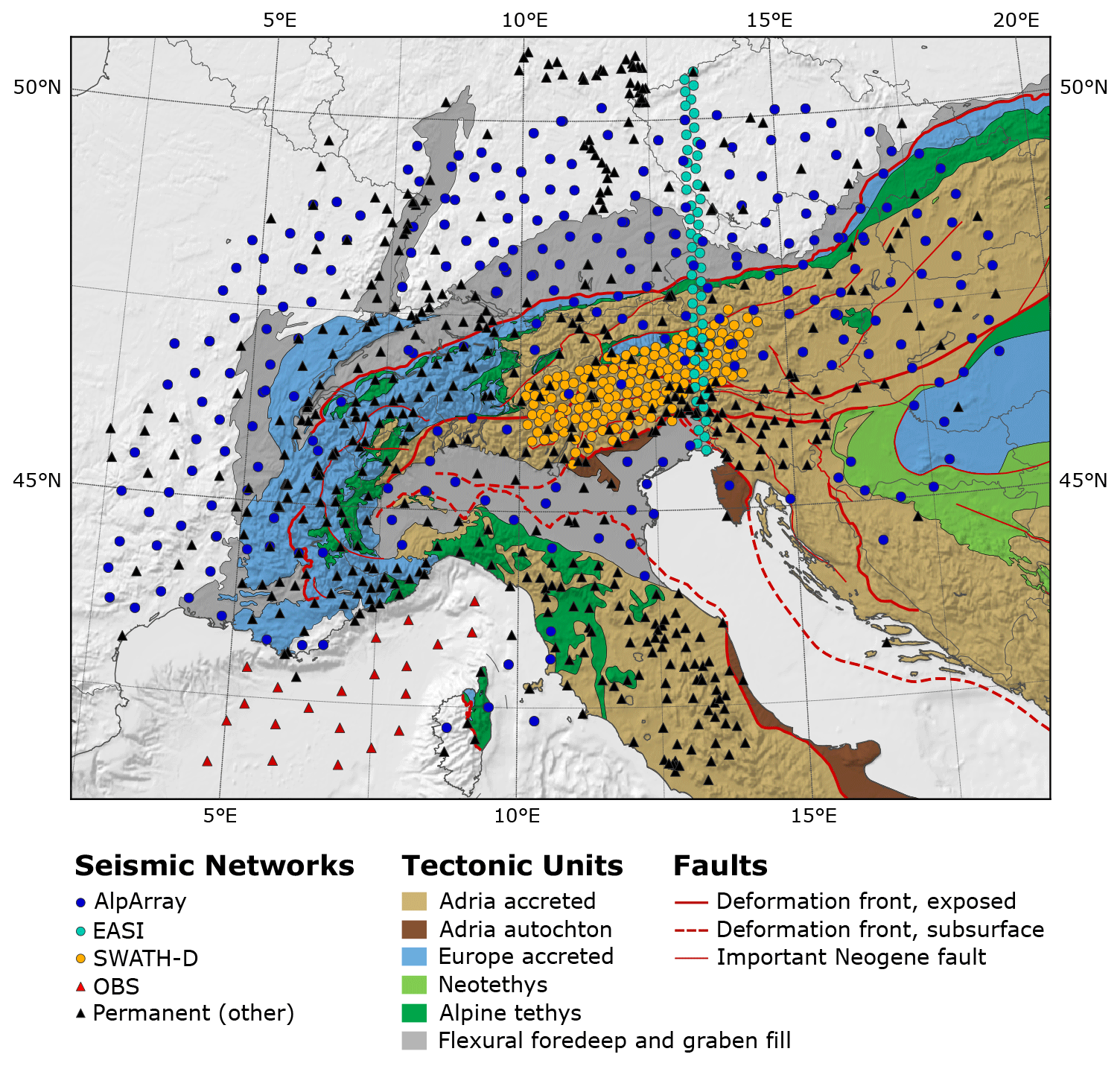
Figure 1 Tectonic map of the Alpine chains compiled by Handy (2021) showing different seismic networks and temporary experiments, tectonic units and major fault systems. Tectonic units and major lineaments simplified from Bigi et al. (1990), Schmid et al. (2004, 2008), Froitzheim et al. (1996), Handy et al. (2010) and Bousquet et al. (2012).

To tackle the challenging research opportunities offered by the AlpArray data with regard to Alpine mantle structure, travel-time tomography of teleseismic body waves certainly belongs to the methods of choice (e.g. Mitterbauer et al., 2011; Lippitsch et al., 2003). In teleseismic tomography, the variation of arrival times of body waves from distant earthquakes across the array are inverted for velocity perturbations below the array (e.g. Aki et al., 1977). Models obtained with this technique using regional arrays are typically confined to the upper mantle. For the AlpArray Seismic network the lower bound is around 600 km depth. Assuming a spherical chunk with a lateral extension similar to that of the seismic array (up to ∼10^∘), below this depth only about one-fourth of the horizontal area spanned by this chunk is penetrated by intersecting rays, leading to smearing of anomalies along the rays within the remaining area (e.g. Sandoval et al., 2004). Lateral resolution is limited by the station spacing of the array. The method is mainly sensitive to volumetric perturbations of seismic velocity and does not give constraints on the location of internal discontinuities. It has been used in many studies on mantle structure, for example Koulakov et al. (2002), Lippitsch et al. (2003), and Piromallo and Morelli (2003).

A method which reaches beyond teleseismic tomography is full waveform inversion (FWI), where entire or partial waveforms are inverted for velocity and also density perturbations (e.g. Mora, 1987; Tromp et al., 2005; Fichtner et al., 2009; Zhu et al., 2012, 2015; Butzer et al., 2013; Schumacher et al., 2016). Predictions of waveforms for given velocity models are obtained by full 3D numerical forward modelling, making the method very expensive with regard to storage requirements and computation time. When applied to teleseismic body waves, hybrid approaches are invoked to make the method numerically tractable (e.g. Monteiller et al., 2013; Tong et al., 2014a, b): full 3D forward modelling is only done in a regional box below the array while wave propagation from the distant earthquake to this box is done by less expensive methods which, however, assume laterally homogeneous or axially symmetric earth structure.

One basic preparatory step for both methods is the determination of travel times. While the need for travel times is obvious for travel-time tomography, teleseismic full waveform inversion can also benefit from travel times in two different ways. First of all, FWI requires a good (ideally 3-D) starting model to ensure that the inversion converges to the global minimum. This model can be obtained from a travel-time tomography. Secondly, since the waveforms are typically band-passed to some (narrow) frequency range, they become monochromatic and waveform matching may suffer from cycle skipping. In such a situation, absolute travel times as additional constraints can help to make waveform matching less ambiguous. Traditionally, arrival times were determined by manual reading of onset times from seismic records, but it is well-known that even manual readings are affected by different reading styles of analysts (e.g. Douglas et al., 1997; Diehl et al., 2009b) and, hence, may suffer from substantial inconsistencies. Moreover, manual reading of hundreds of thousands of records would require an unfeasible amount of human effort. To cope with the ever increasing number of available seismic stations, automatic procedures have been developed to determine arrival times.

One of the first automatic picking procedures that is still used as a fast signal detection method was introduced by Allen (1978, 1982). It is based on a characteristic function (CF) which is calculated as the ratio of the average of a signal within a short time window to that in a long time window (STA/LTA). The CF rises as soon as a signal with a higher amplitude than the preceding noise is encountered in the short time average window. Baer and Kradolfer (1987) developed an automatic phase picker by modifying Allen's characteristic function and implementing a dynamic threshold. The algorithm developed by Küperkoch et al. (2010) modifies and applies the scheme of Saragiotis et al. (2002). Kurtosis or skewness of a seismogram is calculated in a moving window, and the Akaike information criterion (Akaike, 1971, 1974) is applied to the resulting CF.

These approaches work well in the context of local to regional scales and have been used for earthquake location and local earthquake tomography methods. In case of similar waveforms, e.g. from earthquake clusters or teleseismic waves, one can improve travel-time measurements by cross-correlation of waveforms (e.g. Rowe et al., 2002; Mitterbauer et al., 2011). Especially in view of the newly available dense seismic arrays and our quest for ever improving spatial resolution of tomographic models, the accuracy of travel-time measurements plays an increasingly important role. Correlation techniques have been developed where selected wave packets of two different records of similar waveforms are correlated to determine their relative time shift. VanDecar and Crosson (1990) developed a multi-channel cross-correlation (MCCC) technique to obtain high-precision relative arrival times by correlating each trace with every other. This method was also used in a recent study by Zhao et al. (2016) where a finite-frequency kernel method was used for a tomography of the central European subsurface. However, this method does not produce absolute arrival times, which are a prerequisite for the stabilisation of the FWI.

In this paper, we confirm that even advanced techniques of automatic reading of arrival times do not reach the accuracy required by teleseismic travel-time tomography on dense arrays. Using AlpArray data, we demonstrate that an appropriate combination of automatic picking, correlation measurements and beamforming can attain the required accuracy and provide both reliable travel-time residuals and absolute travel times. Applying this technique, we are able to map the propagation of P wave fronts across the AlpArray network and to obtain sufficiently accurate travel-time residuals at all stations of the network. By analysing records of hundreds of teleseismic earthquakes, we can show the coherency and reproducibility of the residuals and study their dependency on event azimuth and frequency. Stacking of event-specific travel-time residuals yields very stable patterns that already indicate the approximate location of high- and low-velocity anomalies in the upper mantle prior to any tomographic inversion. We shall use these time measurements in a later study for performing a teleseismic tomography and full waveform inversion.

2 Data basis

Deployment of temporary stations of AlpArray backbone network Z3 was started in 2015 (Fig. 1) and continued until summer 2016 when the maximum number of 256 temporary broadband stations was reached. From June 2017 to February 2018, 24 ocean bottom seismometers were deployed in the Ligurian Sea by the LOBSTER and the AlpArray-FR project. The earliest complementary experiment, partly included in our dataset, is the Eastern Alpine Seismic Investigation (EASI) project with 55 stations deployed on a north–south profile at 13.4^∘ E, crossing the Alps from the northern Alpine foreland to the Adriatic Sea, which recorded ground motions for more than a year until August 2015. The second complementary experiment SWATH-D was carried out for 2 years starting at the end of 2017, further increasing station density in a key area of the central and eastern Alps, directly above a Moho offset (TRANSALP Working Group, 2002; Spada et al., 2013), a possible slab gap and slab polarity switch (Lippitsch et al., 2003), thereby adding another 154 seismic broadband stations to our dataset. Finally, we extended the coverage of our database to the north and south by adding permanent stations in central Germany and northern Italy, thus obtaining a total of 1025 different seismic broadband stations with recording times scattered through a period of over 4.5 years between 2015 and the end of 2019, with a peak in-station coverage of more than 720 stations in late 2017.

2.1 Teleseismic tomography database

From the available data described above, we assembled records suitable for teleseismic tomography from 974 teleseismic earthquakes with origin times between January 2015 and July 2019 and moment magnitude 5.5 or higher. They encompass waveforms of all stations available in a 5^∘ radius around a central position in the Alps located at 46^∘ N and 11^∘ E. Out of these we evaluated mantle phases for 765 events, all within distances between 35 and 135^∘ relative to the central position, leading to a minimum event distance of 30^∘ for the closest and a maximum event distance of 140^∘ for the farthest station. Information on location and moment tensor was taken from the Global CMT catalogue distributed by the Lamont-Doherty Earth Observatory (LDEO) of Columbia University (Dziewonski et al., 1981; Ekström et al., 2012).

We produced a high-frequency dataset (db_0.5) using a fourth-order Butterworth band-pass filter between 0.03 and 0.5 Hz, which turned out to be perfectly suited for combining automatic picking and cross-correlation of land station records. Because oceanic microseismic noise is rather strong in this frequency band, cross-correlation of OBS records was only possible for earthquakes with magnitudes above 6.2 to 6.5 depending on epicentral distance. For this reason, we assembled a second, low-frequency dataset (db_0.1) with band-pass-filter upper-corner frequency of 0.1 Hz. In this way, most of the oceanic microseismic noise could be avoided, though at the expense of pick accuracy and resolution of teleseismic tomography.

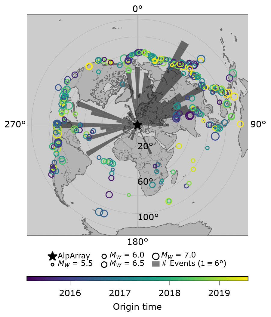
Figure 2 Event distribution of the high-frequency dataset db_0.5. Size of circles correlates with moment magnitude, colour with origin time. Histogram shows number of events binned in 5^∘ bins azimuthally. A bar height of 60^∘ radial distance equals 10 events coming from that direction. The distribution is very irregular with most events located in the northeastern quadrant and in a western sector. There are large gaps with few or no events especially from the southeast as well as from the northwest. Peak value is 18 events for the back-azimuth interval between 30 and 35^∘.

The distribution of earthquakes of both datasets relative to the Alps strongly varies with azimuth and epicentral distance. Figure 2 shows the distribution of 370 events that were ultimately picked for the high-frequency dataset. The signal-to-noise ratio of the waveforms from the remaining events was too low owing to either an unfavourable magnitude-to-distance ratio or radiation pattern. The majority of the recorded waves reach the Alps from a sector between north and east (0 to 90^∘) mainly originating from the Pacific Ring of Fire at epicentral distances between 80 and 90^∘. A second concentration of sources in a sector between WSW and WNW with azimuths between 230 and 290^∘ is produced by earthquakes in the subduction zones of North and South America. Epicentral distances in this sector are more broadly distributed than in the NE sector. There is a remarkable lack of events in a sector between about 100 and 230^∘ as well as in the opposite direction between 290 and 340^∘. To obtain at least a few usable records from the poorly covered sectors long recording periods are essential.

3 Automatic determination of absolute travel times, travel-time residuals and uncertainties

In the following part, we will examine the capability of characteristic functions to resolve travel-time residuals with an accuracy required for high-resolution travel-time tomography. We will summarise the most prominent difficulties and demonstrate how we can benefit from a combination of the AIC algorithm, beamforming and cross-correlation. The resulting multi-stage algorithm combines theoretical onset calculation for spherically symmetric earth models, characteristic functions and various steps of signal cross-correlation and beamforming to obtain absolute as well as relative onsets with an uncertainty of fractions of a second. We also present an empiric way of automatic evaluation of uncertainties which has proven to be extremely robust.

3.1 Definitions and methodological approach

In the following, we will use the quantities absolute travel time at some station, τ_j, defined as the absolute arrival time minus source time; theoretical travel time, T_j, defined as the time relative to the earthquake source time predicted by a standard earth model using an available earthquake location; and averages of these quantities over the entire array, $\stackrel{\mathrm{‾}}{\mathit{\tau }}$ and $\stackrel{\mathrm{‾}}{T}$, respectively. The travel-time residual is defined by

$$\begin{array}{}\text{(1)}& r_j={\mathit{\tau }}_j-T_j-(\stackrel{\mathrm{‾}}{\mathit{\tau }}-\stackrel{\mathrm{‾}}{T})={\mathit{\tau }}_j-\stackrel{\mathrm{‾}}{\mathit{\tau }}-(T_j-\stackrel{\mathrm{‾}}{T}).\end{array}$$

We subtract array averages of observed and theoretical travel times to form residuals, because pure differences between the two quantities contain errors of source time and depend on the wave path through the entire earth. The difference between the array averages, $\stackrel{\mathrm{‾}}{\mathit{\tau }}-\stackrel{\mathrm{‾}}{T}$, should absorb most of the heterogeneous earth structure remotely from the array, while the remaining residuals after average subtraction should rather reflect influences of heterogeneities below the array.

Highly accurate travel times and travel-time residuals are obtained as follows: first a very low-noise beam trace associated with some selected reference station is constructed by stacking appropriately shifted waveforms of all or selected stations on top of the reference station trace. Then, cross-correlation of the beam trace with all other traces is performed to determine highly accurate time lags relative to the beam. Finally, a travel time is read from the low-noise beam trace itself using automatic picking. Let us denote the beam travel time by τ_B and the time lag of station j relative to the beam by Δτ_jB. Then, absolute travel time and its array average are given by

$$\begin{array}{ll}{\displaystyle }{\mathit{\tau }}_j& {\displaystyle }={\mathit{\tau }}_{\mathrm{B}}+\mathrm{\Delta }{\mathit{\tau }}_{j\mathrm{B}},\\ \text{(2)}& {\displaystyle }\stackrel{\mathrm{‾}}{\mathit{\tau }}& {\displaystyle }={\mathit{\tau }}_{\mathrm{B}}+\stackrel{\mathrm{‾}}{\mathrm{\Delta }\mathit{\tau }},\end{array}$$

where $\stackrel{\mathrm{‾}}{\mathrm{\Delta }\mathit{\tau }}$ denotes the array average of the time lags relative to the beam. The travel-time residual is given by

$$\begin{array}{ll}{\displaystyle }{r}_j& {\displaystyle }={\mathit{\tau }}_j-\stackrel{\mathrm{‾}}{\mathit{\tau }}-(T_j-\stackrel{\mathrm{‾}}{T})\\ {\displaystyle }& {\displaystyle }={\mathit{\tau }}_{\mathrm{B}}+\mathrm{\Delta }{\mathit{\tau }}_{j\mathrm{B}}-{\mathit{\tau }}_{\mathrm{B}}-\stackrel{\mathrm{‾}}{\mathrm{\Delta }\mathit{\tau }}-(T_j-\stackrel{\mathrm{‾}}{T})\\ \text{(3)}& {\displaystyle }& {\displaystyle }=\mathrm{\Delta }{\mathit{\tau }}_{j\mathrm{B}}-\stackrel{\mathrm{‾}}{\mathrm{\Delta }\mathit{\tau }}-(T_j-\stackrel{\mathrm{‾}}{T}).\end{array}$$

Note that the travel-time residual is independent of the beam travel time and, hence, its accuracy is fully determined by the accuracy of the time lags Δτ_jB.

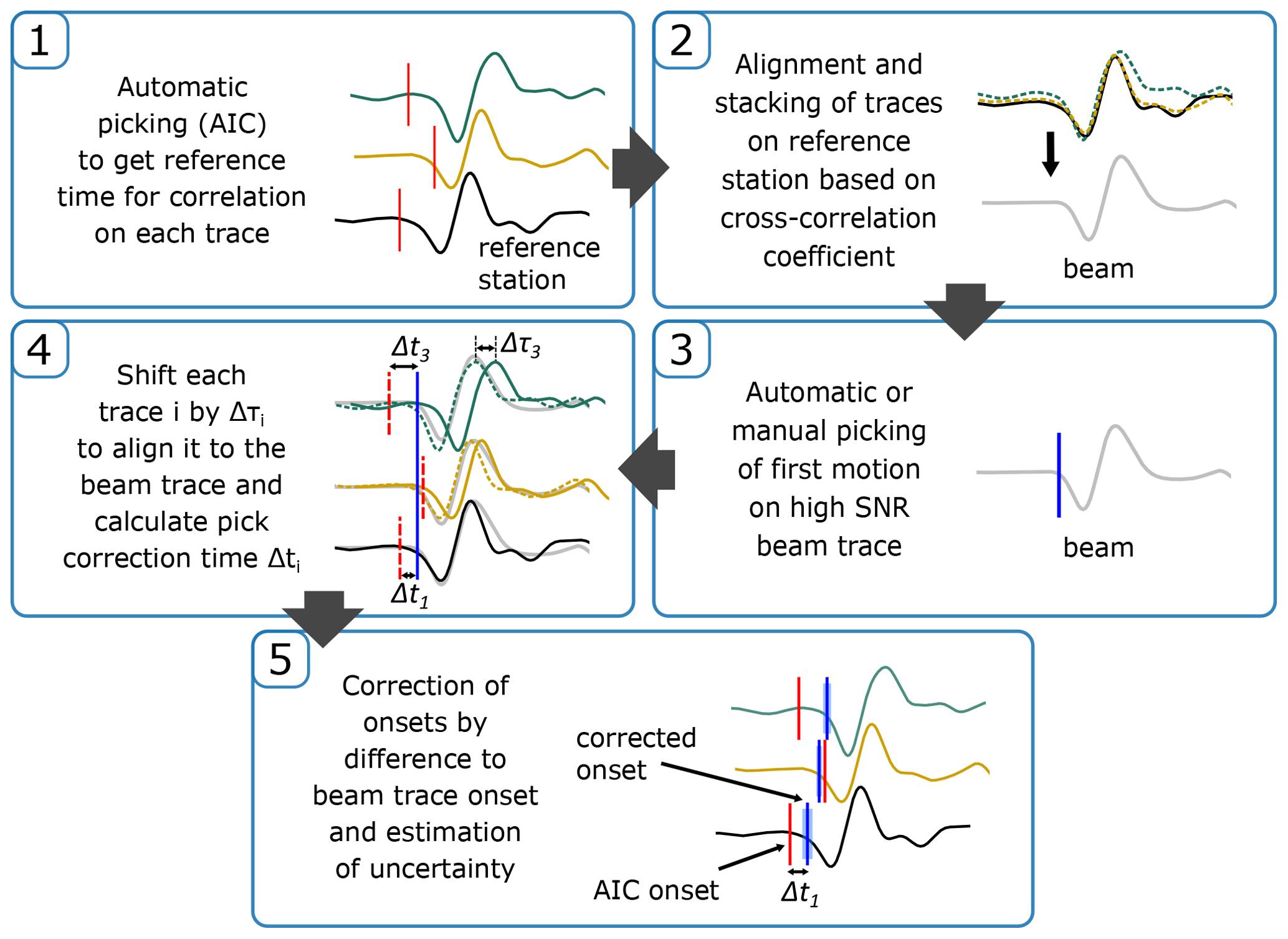
Figure 3 Workflow of the correlation picking algorithm. Solid lines show exemplary waveforms on three different stations. Black solid line shows reference station trace. Dashed lines of waveforms indicate that a waveform has been cut and shifted onto the reference (or beam) trace. Red vertical lines show reference AIC onset times, blue solid lines show corrected onsets.

To obtain the beam itself, we first select a reference station and consider travel-time differences to all other stations, τ_j−τ_R, which are again determined by cross-correlation. The reference station should be close to the centre of the array to minimise waveform discrepancies to other stations and exhibit a high data availability and low noise. We then use these time differences to shift the station traces and stack them on top of the reference trace to form the beam. Stacking is restricted to traces with sufficiently high correlation with the reference trace. To perform these initial cross-correlations efficiently, we take advantage of automatic readings at the stations based on higher-order statistics and the Akaike information criterion (Küperkoch et al., 2010). The complete workflow is illustrated in Fig. 3.

3.2 Higher-order statistics picking algorithm

To get initial P wave onsets as reference times for cross-correlation in records of teleseismic earthquakes we use the HOS/AIC algorithm by Küperkoch et al. (2010), which was originally designed for precise local to regional earthquake detection, location and focal mechanism estimation but not for teleseismic phase reading. Therefore, all wavelength-dependent parameters were adapted to our needs.

We choose kurtosis, the central moment of order 4, as the characteristic function, which is calculated on a mean removed seismogram in a moving window of N time samples at index j as

$$\begin{array}{}\text{(4)}& {\widehat{m}}_{\mathrm{4}}\left(j\right)={\displaystyle \frac{\mathrm{1}}{N}}\sum _{l=\mathrm{0}}^{N-\mathrm{1}}{x}_{j-l}^{\mathrm{4}}.\end{array}$$

The AIC, which estimates the information loss of a function, is applied to the kurtosis function in the following way (Küperkoch et al., 2010):

$$\begin{array}{ll}{\displaystyle }\text{AIC}\left(k\right)=& {\displaystyle }(k-\mathrm{1})\lg \left({\displaystyle \frac{\mathrm{1}}{k}}\sum _{j=\mathrm{1}}^k{m}_{\mathrm{4}}(j{)}^{\mathrm{2}}\right)\\ \text{(5)}& {\displaystyle }& {\displaystyle }+(L-k+\mathrm{1})\lg \left({\displaystyle \frac{\mathrm{1}}{L-k+\mathrm{1}}}\sum _{j=k}^L{m}_{\mathrm{4}}(j{)}^{\mathrm{2}}\right),\end{array}$$

with L being the length of the kurtosis function and k ranging from 0 to L.

As initial guess, we use theoretical onsets of the phase estimated for a spherically symmetric earth model and calculate characteristic functions in a properly chosen time window around those onsets. The most probable pick (mpp) is defined as the minimum of the AIC of the phase in this window. We select the moving time window a full order of magnitude larger than those typically used for local earthquake onset determination and calculate the most probable onset. Subsequently, an automatic quality is assigned to the onset based on the signal-to-noise ratio and the difference between the latest and earliest possible pick (Diehl et al., 2009b). This quality determines whether the pick is used for further processing. The earliest possible pick, t_epp, is calculated as half the signal period before the most probable pick, t_mpp, accounting for a possibly missed first oscillation before the most probable pick. The signal period for this step is estimated by the mean time differences of zero-crossings within a characteristic time window after the most probable pick. The latest possible pick, t_lpp, is set to the time where the signal amplitude exceeds the noise level which is calculated as the root mean square of the noise in a window preceding the most probable pick. A symmetrised pick error (SPE) is then calculated as a weighted average of both pick uncertainties with double weight on the uncertainty derived from the latest possible pick:

$$\begin{array}{ll}{\displaystyle }\text{SPE}& {\displaystyle }={\displaystyle \frac{\mathrm{\Delta }{t}_{\text{earliest}}+\mathrm{2}\mathrm{\Delta }{t}_{\text{latest}}}{\mathrm{3}}}\\ {\displaystyle }& {\displaystyle }={\displaystyle \frac{(t_{\text{mpp}}-t_{\text{epp}})+\mathrm{2}(t_{\text{lpp}}-t_{\text{mpp}})}{\mathrm{3}}}\\ \text{(6)}& {\displaystyle }& {\displaystyle }={\displaystyle \frac{\mathrm{2}{t}_{\text{lpp}}-t_{\text{epp}}-t_{\text{mpp}}}{\mathrm{3}}}.\end{array}$$

By definition, using a maximum frequency of 0.5 Hz, we obtain a minimum uncertainty from the earliest possible pick of a full second. Assuming Δt_latest=0, the minimum possible SPE will be 0.33 s. However, more realistic uncertainties will likely range of the order of 1 to 2 s close to the maximum travel-time residuals expected from mantle heterogeneities below the Alpine orogen. We will show later (Fig. 5a) that in many cases pick uncertainties even exceed typical travel-time residuals of interest. To resolve the fine-scale mantle structure below the Alps, it is crucial to reduce the uncertainties of the onsets using additional constraints provided by the high station density of the AlpArray network.

By visual inspection of selected examples, we validated that the large uncertainties result from difficulties of the characteristic function algorithm to find that part of the first P wave onset which is similar in all traces. The reason for this is the relatively low amplitude of the P onset which is often hidden in site-specific noise. The resulting most probable onsets therefore strongly scatter, confirming estimated uncertainties of about one half of the signal period. Another limitation of the characteristic function approach is the false picking of either later-arriving phases due to the first motion being completely masked by noise or of other signals produced in the vicinity of the station leading to a severe number of outliers and to a time-intensive manual postprocessing.

Although too uncertain to be used for tomographic inversion, the AIC onsets turned out to be more precise than onsets predicted with standard 1D earth models and are therefore better suited as reference times for signal cross-correlation. We found that theoretical phase onsets can differ from actual arrivals by up to some tens of seconds, most probably owing to differences of the true physical properties in the global earth from those of the spherically symmetric earth model, uncertainties in origin time, dispersion processes along the travel path and the use of centroid times of the gCMT catalogue as earthquake origin times (which we want to use for the FWI). The resulting need for large cross-correlation shifts to catch all overlapping phases would involve a high risk of cycle skipping.

An analysis of the necessary shift in travel times predicted by the standard earth model AK135 (Kennett et al., 1995) for the final picks of 370 events in a frequency band between 0.03 and 0.5 Hz yielded an average value of −3.71 s, implying that the average travel time in the area of study is less than that predicted by the AK135 earth model. The standard deviation is σ=5.84 s. We found an absolute time shift of over 10 s for 22 events with a peak value of −53 s. Hence, it is not reasonable to directly use 1D theoretical onsets as starting points for a signal cross-correlation.

Especially for lower-magnitude events and high-noise OBS records it may happen for some stations that useful automatic picks are not available. Provided that there are sufficient records left with a reliable automatic pick, we go back to theoretical travel times as correlation reference times which have been corrected by the median time difference between the available automatic picks and the corresponding theoretical travel times. In this way, we still obtain good time references for cross-correlation and avoid omitting all records with unreliable automatic picks. This approach can greatly increase the number of picks obtained with the cross-correlation technique.

3.3 Correlation approach

Applying a cross-correlation method to improve first arrivals on a large regional array like the AlpArray seismic network is based on the hypothesis of a high similarity of the waveforms of the selected phase across the array. We found this requirement to be satisfied especially well for teleseismic P waves travelling through the mantle but not for PKP phases that penetrate the core. In contrast to mantle P phases, PKP phases are composed of several arrivals which modify the shape of the waveform across the array owing to the different epicentral distances, making signal correlation challenging.

We start by searching for a reference station which represents the waveforms of the entire array best for each single event. The most important criterion for such a station is a continuous operation with high data quality. Therefore, we only consider permanent stations with low noise that were ideally running for the entire time span of events in our database. Also, we want this station to be in a central position in the Alps within the shortest possible distance to all other stations to minimise possible changes in waveform related to large-scale heterogeneities in the global earth (see Sect. 3.1). For each event we start with a small pool of stations meeting those criteria and correlate the signals of all other stations in small time windows around the reference times we get from the AIC picks and the corrected theoretical travel times. The reference station with the highest mean correlation is then chosen to be representative of the full set of stations for this event. Combining each station selected as reference for an event with all other available stations leads to 187 000 correlation pairs for the 370 events in our database. The average cross-correlation coefficient for those signal pairs is 0.78.

After correlating all stations with the reference station, we align the waveforms according to the time of the maximum of the cross-correlation function. For each event we then form a beam representing the onset of the first P wave phase by stacking the vertical component traces onto the reference station if the maximum cross-correlation coefficient is ≥0.8 (Fig. 3). To find the exact time of highest correlation independent from sampling, a parabola is fitted around the concave part of the cross-correlation function and analytically evaluated for its apex (Deichmann and Garcia-Fernandez, 1992).

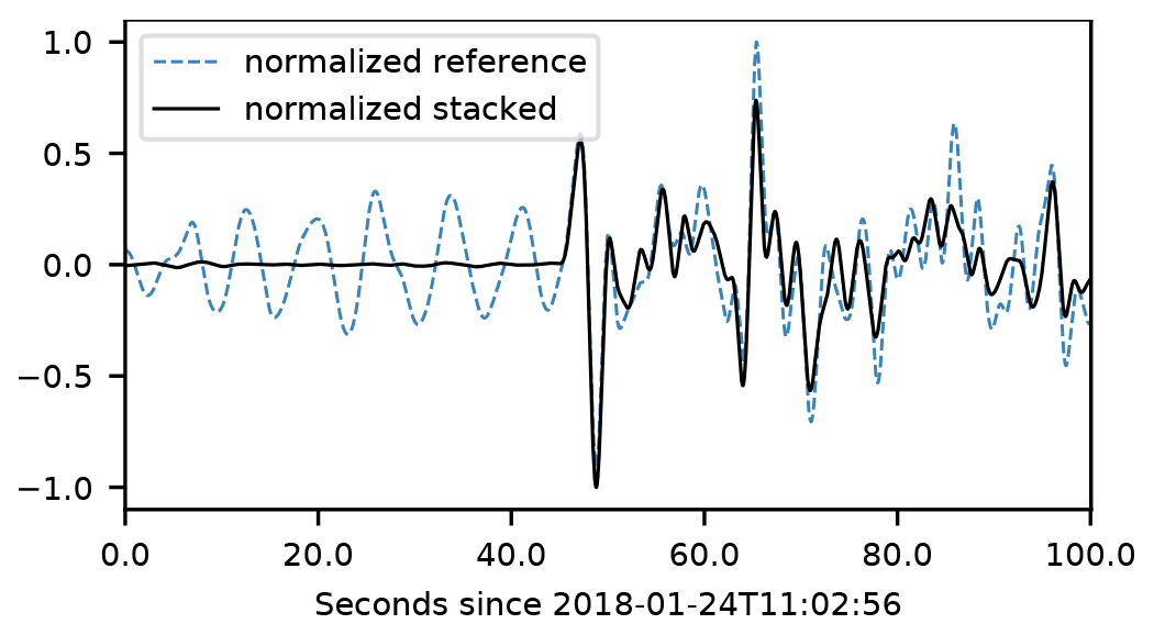
Figure 4 Stacking example for M6.1 earthquake in Hokkaido, Japan, on 24 January 2018. Out of a total of 746 stations with a cross-correlation coefficient >0.8 to the reference trace CH.PANIX (blue line), 450 are stacked onto each other (black line). The first motion that was poorly resolvable on the reference trace can be clearly identified on the stacked trace, as the signal-to-noise ratio increased by a factor of 30 in the stacking process. Both traces are normalised for comparison and filtered between 0.03 and 0.5 Hz.

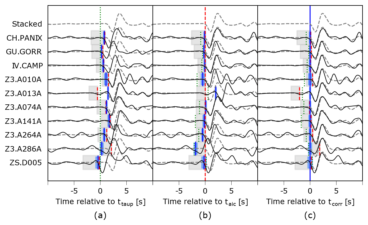
Figure 5 Waveform fit for P arrivals of a M5.6 event on 7 August 2018 using the beam waveform as reference (dashed line). (a) Traces of different exemplary stations aligned by their theoretical onset (green dotted line). Travel-time residuals (not demeaned) for each trace can be read from the differences of AIC (red dashed line) and correlation onsets (blue solid line) to the theoretical onset. Onset uncertainties are displayed by shaded areas in grey (for absolute AIC onsets) and blue colours (for relative onsets based on cross-correlation), respectively. There is a good agreement between AIC and correlation-based onsets; however, the estimated absolute uncertainty of the AIC onsets is large, often exceeding the residual to the theoretical onset. (b) Alignment of traces by their AIC onset. Overlap with the beam trace is good but fails in certain cases of higher noise, which can lead to AIC onsets that are too early (e.g. Z3.A013A) as well as too late (e.g. Z3.A286A). (c) Alignment by the correlation-corrected onsets. Overlap with the beam trace is close to ideal. The estimated uncertainty of correlation-corrected onsets is by a factor of about 10 lower than that of the AIC picks. Note the increased uncertainty for trace ZS.D005 and Z3.A010A exhibiting significant coda.

The resulting beam (Fig. 4) is of very high quality with an increase in signal-to-noise ratio (SNR) by a factor of about 30. On the beam, first motion becomes clearly visible and can be determined precisely either automatically or manually. In our case, we applied the automatic picking procedure of Sect. 3.2 to determine the onset on the beam trace. Alternatively, the reference onset can be determined by hand once for each event. After determination of the absolute pick on the beam, vertical components of all stations are correlated with it. The travel time at each station is then calculated as the beam travel time plus the time difference obtained from the lag time associated with the maximum correlation between the beam waveform and the waveform at the station. After onset determination our algorithm also searches for outliers within a time window around an expectation value we calculate for each station to further assess possible cycle-skipping issues. Finally, to assure the consistency of our travel-time dataset, wave fronts are constructed and visually inspected. Outliers can be easily recognised as they create strong distortions of the travel-time isochrones.

The different role of theoretical, AIC and correlation-corrected travel time is illustrated in Fig. 5. If the traces are aligned according to theoretical travel time (Fig. 5a), the alignment with the beam trace is the worst. Evidently, this must be due to lateral heterogeneities below the array not contained in the standard earth model. If the traces are aligned according to their AIC automatic pick (Fig. 5b), overlap with the beam trace improves, but there are still significant deviations, for example for stations Z3.A013A and Z3.A286A. The agreement with the stacked trace is best when the traces are aligned according to their correlation-corrected onsets. Fig. 5c demonstrates the scatter of the AIC picks which makes them insufficient for teleseismic tomography.

3.4 Error estimation

Estimating an error for automatically determined as well as for manually assigned travel times is a difficult task and can be rather subjective. The concept of earliest and latest possible pick for error estimation uses information of a single trace only and is not suited for travel-time residuals determined by cross-correlation, as the credibility of a time difference to a reference trace associated with a high cross-correlation coefficient is by far higher. This argument also applies for uncertainties of the absolute onsets, if the reference trace is a low-noise beam where the concept of estimating the earliest possible pick as half the signal wavelength is questionable, as the first onset may be clearly identifiable without any risk of missing the first oscillation.

As the beam represents the waveform of the majority of stations, we consider the maximum cross-correlation between station and reference trace as the most important indicator for the relative accuracy of a travel-time difference. However, this assumption only holds if the stations forming the beam trace are evenly distributed in the array and not just representing a part of the array (for example stations close to the reference station). This is vital for the consistency of the full dataset.

Moreover, using the cross-correlation coefficient as a measure of accuracy might lead to a down-weighting of traces of stations influenced by strong local heterogeneities whose waveform does not fit the shape of the reference trace. Fortunately, this matter can be easily identified by looking at spatial distributions of maximum correlation. Affected stations should stand out in comparison to adjacent stations when looking at correlation coefficients averaged over many events (Sect. 4). We tried to find such regional dependencies by creating spatial plots of the cross-correlation coefficient for randomly selected events but could find neither evidence of a decrease in the correlation coefficient with distance to a reference station nor regional clusters of high or low cross-correlation coefficients.

A second criterion for a good match of station and reference trace is the shape of the cross-correlation function itself. Hence, we also evaluate the full width at half-maximum (FWHM) of the cross-correlation function. If the FWHM increases, the cross-correlation maximum loses sharpness and the accuracy of a travel-time difference decreases. This approach implies a frequency dependency of travel-time uncertainty, leading to a higher uncertainty for longer periods (and hence wavelengths).

For a parabola fitted to the maximum of the cross-correlation function of the form

$$\begin{array}{}\text{(7)}& f\left(x\right)=a{x}^{\mathrm{2}}+bx+c,\end{array}$$

the full width at half maximum (FWHM) can be calculated as

$$\begin{array}{}\text{(8)}& \text{FWHM}=\mathrm{2}\sqrt{{\left({\displaystyle \frac{b}{\mathrm{2}a}}\right)}^{\mathrm{2}}+{\displaystyle \frac{C_{max}-\mathrm{2}c}{\mathrm{2}a}}},\end{array}$$

where C_max denotes the maximum correlation. To combine both criteria, we chose to calculate the travel-time difference uncertainty as follows:

$$\begin{array}{}\text{(9)}& \mathit{\sigma }=(\mathrm{1}-C_{max})\text{FWHM}.\end{array}$$

The influence of a bad fit owing to signal coda on the cross-correlation coefficient and hence travel-time residual uncertainty is illustrated in Fig. 5c. The contribution of the width of the cross-correlation function, depending on signal period, is practically the same for all traces of this event. However, the maximum correlation decreases for stations with additional complexity in the signal (ZS.D005 and Z3.A010A).

4 Uncertainties of travel-time residuals

We categorise travel-time uncertainties into five different classes in steps of 0.1 s ranging from class 0 (best), below 0.1 s, to class 4 (worst), over 0.4 s. Although there is only a lower bound of the uncertainty for class 4, each onset in this class still has a well defined uncertainty and could in principle be used for tomography. Comprising over 170 000 onsets, the travel-time uncertainty distribution of db_0.5 (Fig. 6a) has a maximum at 0.08 s. The median of the distribution is 0.15 s, the mean is 0.2 s. Our average value of the estimated uncertainties is therefore lower than the one estimated by Lippitsch et al. (2003), who report a value of 0.36 s for 4199 P wave travel times, and larger than the one reported by Zhao et al. (2016), who estimate a value of less than 0.1 s for their 41 838 travel-time residuals. However, due to the high number of stations in the AlpArray project, our dataset contains over 46 000 (27 %) of the onsets in the highest class with an estimated uncertainty <0.1 s. Less than 10 % are in the lowest class of 0.4 s or higher.

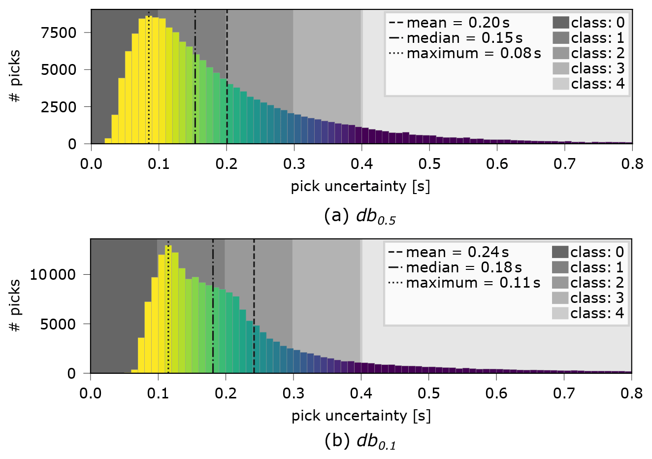
Figure 6 Pick uncertainty distribution of db_0.5 and db_0.1, clipped at 0.8 s. Uncertainties in the histograms are coloured identical to Fig. 7 for an easier comparison.

The low-frequency dataset db_0.1 has an increased signal quality (i.e. higher SNR) (Fig. 6b) which is reflected in the higher number of picks (over 214 000), an increase of over 25 % compared to the high-frequency dataset. However, the travel-time uncertainty distribution is drawn to higher values, with its mean being shifted by nearly half a class towards higher uncertainties. While the peak value of the uncertainty histogram is still in the same region as that of the high-frequency dataset, there are only about 10 % of the total number of picks in class 0 and over 12 % in class 4. The reason for this counter-intuitive behaviour is the fact that, owing to the greater signal periods, the maxima of the correlation function for estimating the time differences (Sect. 3.4) become wider, leading to a higher error estimate.

4.1 Regional distribution

An evaluation of the regional distribution of the median of travel-time uncertainty per station in the db_0.5 dataset (Fig. 7a) exhibits lower values north and east of the Alpine arc, in central and southern Germany, as well as in the Czech Republic, eastern Austria and Slovenia. We hypothesise that this effect originates in the spatial segregation of those areas from the Alpine orogen, as the subsurface structure of the surrounding area of the Alps is simple in comparison to that beneath the Alps. In contrast to that, travel-time uncertainty increases above the highly complex structures in the Alpine arc where the P wave fronts are significantly altered by the strongly heterogeneous subsurface. This decreases their correlation with the waveforms on other stations of the array and to the stacked reference trace. It is also likely that uncertainty increases due to local site effects which can be significant in narrow valleys where anthropogenic activities such as traffic are harder to evade. These influences should be visible on single stations which show a high daytime noise level. We expect those effects to be present equally in both the high- and the low-frequency dataset. However, most of the station outliers we see in one dataset are not present in the other.

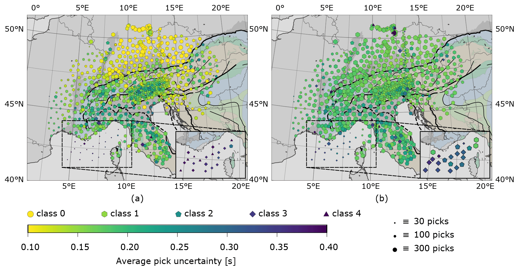
Figure 7 Maps of the median uncertainty of all picks for the high-frequency (a) and the low-frequency (b) dataset. Symbol sizes correlate with number of picks per station, colour shows the average travel-time uncertainty and symbol shapes indicate the average pick class on each station. Inset shows OBS stations only with symbol size increased by a factor of 2.5. Travel-time uncertainty gets higher for db_0.5 in areas strongly influenced by deep subsurface structures, e.g. orogenic roots as well as strong heterogeneities close to the surface. Coverage in terms of measurement duration is best in the northern Alpine foreland, central Alps and Apennines. Complementary experiments are salient, as their measuring duration (i.e. number of total picks) is limited in contrast to other stations. The EASI experiment can be seen as a straight line of smaller-sized symbols on a north–south-directed profile, spatially (but with no overlap in time) cutting through the SWATH-D experiment in the central Alps above the Tauern Window. The latter has a higher station density compared to the rest of the array. Ocean bottom seismometers are characterised by a lower number of picks (smaller symbol size) as well as by a higher average uncertainty as a consequence of their noisy measuring environment.

The travel-time uncertainty distribution pattern of the lower-frequency dataset db_0.1 (Fig. 7b) shows a shape comparable to the high-frequency one with the lowest uncertainty in the northeastern parts of the array. However, overall uncertainty is higher, and the contrast between regions of high and low uncertainty is decreased. We assume that this is an effect of signals of larger wavelengths being less sensitive to small-scale anomalies due to their lower-resolution capability (finite frequency effect) and hence waveform fit with the reference trace being easier to achieve. The only area where we see a totally opposite behaviour is the Ligurian Sea, where the positive impact on pick uncertainty using lower frequencies is salient. Here, not only the number of total picks greatly increased but also average pick quality is raised by a full class for nearly all OBS whilst for the remaining stations quality tends to decrease by almost one class in comparison to the high-frequency dataset. We also note that there are only small changes in uncertainty for the SWATH-D stations. They even show slightly the counterintuitive behaviour of having higher uncertainties than average in db_0.5 but lower uncertainties than average in db_0.1.

The total number of picks per station is highest on permanent station networks which are distributed most densely in the central Alps and Apennines. Temporal coverage decreases slightly in the western part of the Array due to a delayed start of deployment of temporary stations in this area.

5 Regional variation of travel times and travel-time residuals

In the following, we examine the variation of travel times and travel-time residuals across the array, study their dependence on event azimuth and in particular delve into the reproducibility and consistency of the travel-time residuals. In particular, the latter is a crucial prerequisite for a successful tomographic inversion.

5.1 Wave fronts and spatial patterns of travel-time residuals

We start with teleseismic P wave fronts constructed as isolines from the estimated travel times. To further demonstrate the improvement of correlation-corrected travel times over AIC travel times, we show interpolated P wave fronts constructed from both kinds of travel times. As an example, we take the M6.5 earthquake that happened on 17 November 2017 in the Eastern Xizang–India Border Region (Fig. 8). In both cases, one can identify the P wave travelling across the array of about 700 stations from northeast to southwest. However, when constructed from the AIC onsets (Fig. 8a), the wave fronts are strongly irregular and several outliers are apparent, leading to distorted isolines which cannot be explained by mantle heterogeneities. After application of the cross-correlation correction, the resulting wave fronts no longer show the scatter inherent to the AIC onsets and become smooth except for some weak undulations (Fig. 8b). These seem to be produced by several adjacent stations and should be attributed to subsurface structures.

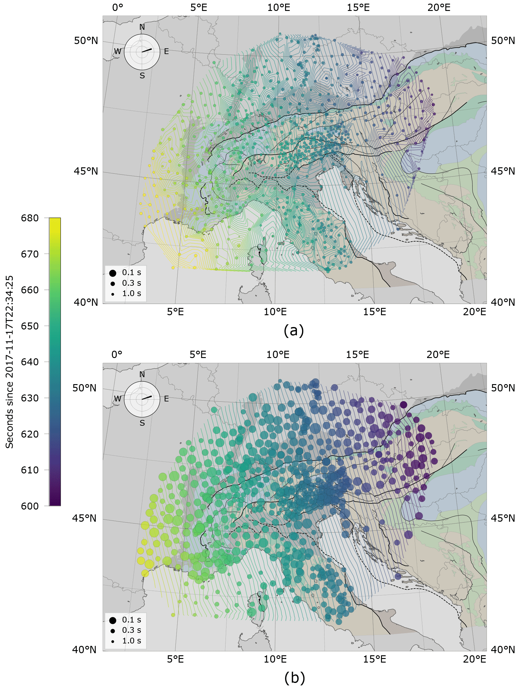
Figure 8 Travel-time fields of the Eastern Xizang–India Border Region event on 17 November 2017. Onsets from (a) the AIC algorithm that were only corrected for severe outliers (noise picks or wrong phases) and (b) the combined cross-correlation AIC algorithm. Onset certainty increases with circle sizes. Isolines are linearly interpolated with isochrone contour intervals of 1 s.

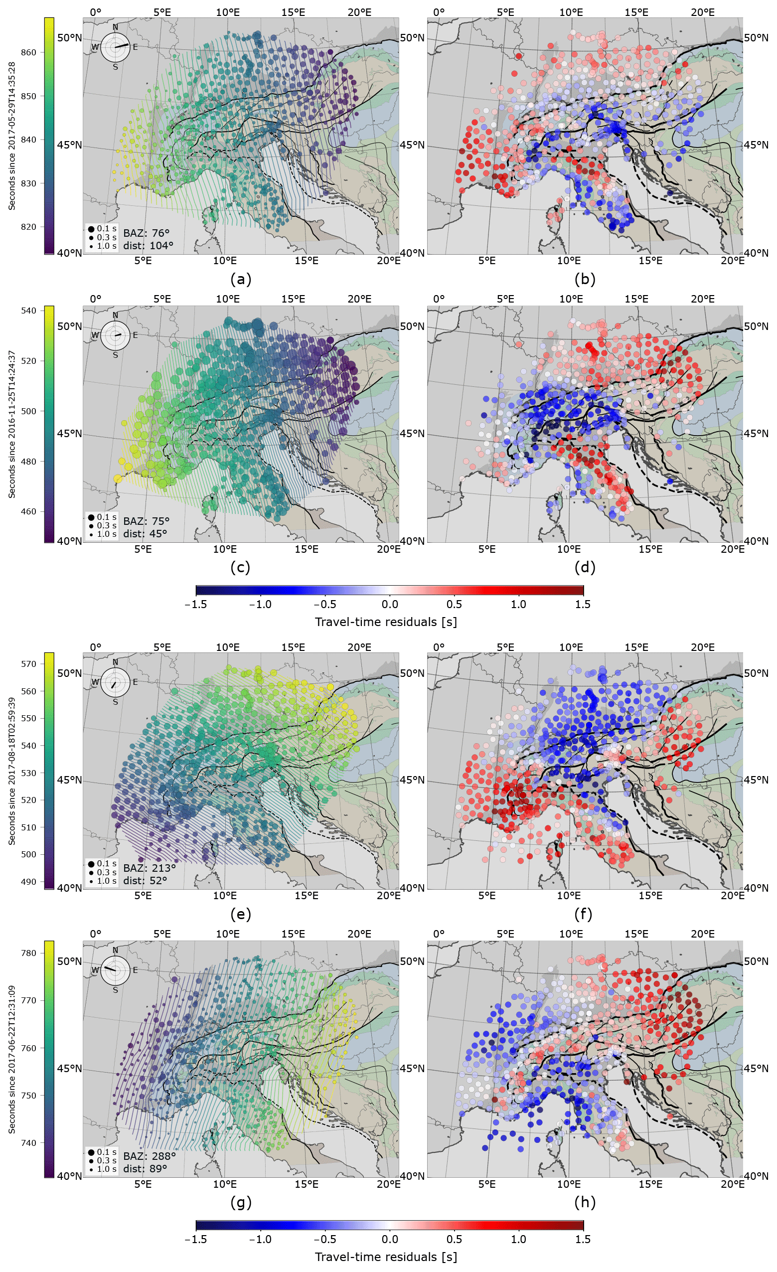
Figure 9 Wave fronts and travel-time residual patterns of different earthquakes. (a, c, e, g) Absolute travel times, distance of isolines 1 s, circle sizes inversely proportional to pick uncertainty. (b, d, f, h) Demeaned travel-time residuals relative to 1D earth model. (a, b) M6.6 event, 29 May 2017, Sulawesi, Indonesia, BAZ=76^∘, distance=104^∘; (c, d) M6.6 event, 25 November 2016, Tajikistan–Xinjiang Border Region, BAZ=75^∘, distance=45^∘; (e, f) M6.8 event, 22 June 2017, near the coast of Guatemala, BAZ=213^∘, distance=52^∘; (g, h) M6.6 event, 18 August 2017, north of Ascension Island, BAZ=288^∘, distance=89^∘.

To illustrate the varying shapes of the wave fronts crossing the AlpArray network from different azimuths and epicentral distances, we have selected four different earthquakes as representative examples: two with nearly equal back-azimuth (75^∘) but very different epicentral distances (104 and 45^∘) and two others covering western (288^∘) and southern (218^∘) back-azimuths with differing epicentral distances (89 and 52^∘) (Fig. ). In addition to the P wave fronts, we show the demeaned travel-time residuals associated with each particular event as defined in Eq. (1). They should correlate with the wave fronts, as deformations of the wave front should lead to travel-time residuals and vice versa. To compensate for the influences of different station elevations, we apply a constant travel-time correction on all residuals shown, assuming vertical propagation and a surface P wave velocity of 5.5 km s⁻¹.

Comparing Fig. a and c reveals a notable difference of the 1 s travel-time isoline spacing which is much greater for the distant event. This reflects the different horizontal apparent velocity of the two wave fields, which is controlled by epicentral distance and is much higher for the more distant event. While the wave fronts are generally regular and smooth, strong distortions become visible in some places. For example, in Fig. a, the spacing of the isolines locally broadens in northern Italy north and east of the Ligurian Sea. This increased spacing can be associated with very large negative residuals beginning at about 7.5^∘ E and 45^∘ N and continuing further to the northeast. The broadening can be explained by the transition from normal to large negative residuals further to the southwest. A second one occurs in the Apennines to the south where the wave front has a strong lag near the western coast of Italy compared to the areas north of it but takes up again while propagating over the areas with negative residuals in the western and central Apennines. In Fig. c, a very similar behaviour is visible.

A closer examination of travel-time residuals shown in Fig. b and d reveals that there is a general agreement between the patterns but also significant differences, for example in southeastern France, where we observe normal to negative residuals for the distant event but positive residuals for the close event. The opposite is the case in most of Switzerland where we observe negative residuals for the close event and rather normal residuals for the distant one. Apparently, the steeply upwards-propagating waves from the distant event see different subsurface structures than the more slanted waves of the close event do.

A comparable behaviour is observed for events arriving from other back-azimuths. Isoline spacing is again much larger for the more distant event whose waves arrive from a WNW direction. In Fig. g, there are again notable distortions of the wave fronts around 7.5^∘ E and 45^∘ N. These distortions are shifted to the NE for the waves arriving from the SSW in Fig. e. The associated residuals exhibit large-scale coherent patterns of negative and positive residuals but are again different in various regions. For example, residuals are generally positive in southeastern France for the waves arriving from SSW while they are normal to negative for the event from WNW. This is again an indication of heterogeneous mantle structure to be resolved by tomography later.

5.2 Stacked residuals

Although travel-time residuals differ with epicentral distance and event back-azimuth as waves move through high- or low-velocity zones from different angles before reaching the surface, there are certain features which tend to occur for a large number of events. The most prominent ones are the negative residuals along the Apenninic and Alpine chain. We stacked residuals for all analysed events to identify regions of stable negative or positive travel-time residuals. It is important to understand that after stacking of the demeaned travel-time residuals, the resulting residuals are relative to an unknown one-dimensional earth model defined by all events used for stacking and not to the standard earth model used to calculate travel-time differences in the first place (e.g. Aki et al., 1977). Hence, negative or positive residuals indicate higher or lower velocities, respectively, relative to this average model and not relative to a standard earth model.

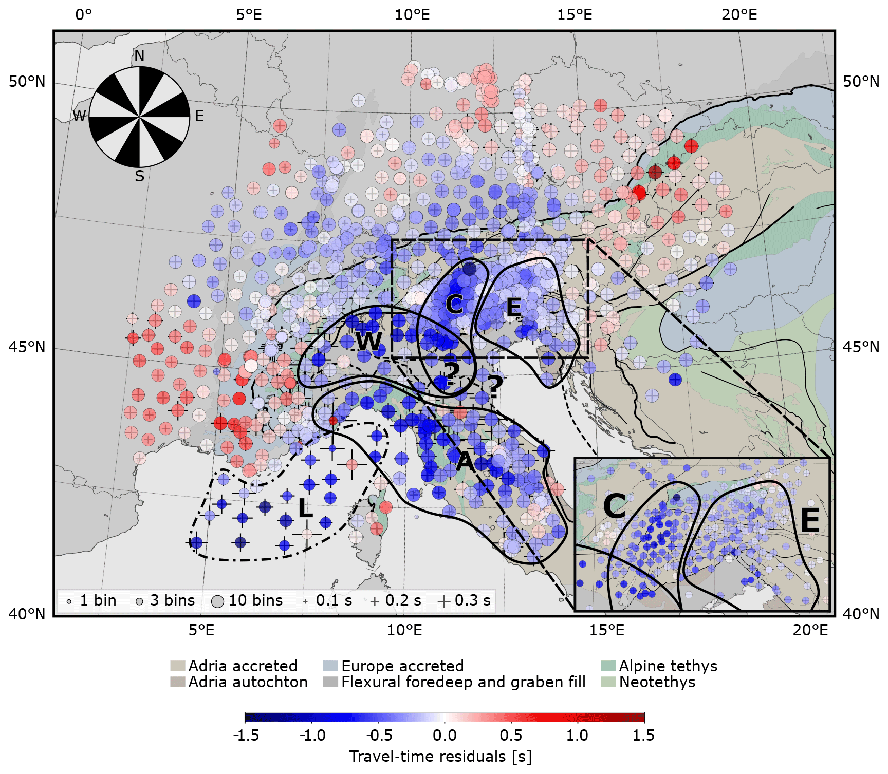
Figure 10 Stacked travel-time differences for 370 events of the high-frequency dataset db_0.5 corrected for crustal influences. Circle sizes correlate with number of back-azimuth bins for each station (maximum=12). Blue colours point to subsurface structures with v_p values higher than average, red colours to structures with v_p values lower than average. Travel times are binned calculating the mean travel time for all events within 30^∘ bins to balance out directional influences. Standard deviation of the azimuthal influence on each station is marked by crosses; e.g. small crosses mark stations residuals mostly independent of variations in back-azimuth. A travel-time correction is applied for the station elevation using a constant near-surface velocity estimate of 5.5 km s⁻¹. High-velocity anomalies are contoured as follows: W – western Alps, C – central Alps, E – eastern Alps, A – Apennines, L – Ligurian Basin. Tectonic map of the Alpine chains compiled by Handy (2021). Tectonic units and major lineaments simplified from Bigi et al. (1990), Schmid et al. (2004, 2008), Froitzheim et al. (1996), Handy et al. (2010) and Bousquet et al. (2012).

As the azimuthal distribution of the events in our database is strongly uneven (Sect. 2.1), it is important to balance out the influence of events from different directions when stacking. Otherwise, the influence of back-azimuths with high event density (e.g. NE in Fig. 2) on travel-time residuals would dominate over data from poorly covered directions. Hence, we create 30^∘ wide back-azimuth bins and, for each station, form a weighted average of all travel-time residuals associated with events in this bin with weights given by the inverse uncertainties of the residuals. The full stack over all events (Fig. ) is finally obtained by averaging over the individual 30^∘ back-azimuth stacks. The value of 30^∘ was chosen as a good compromise between angular resolution and smooth event distribution. The distribution of available measurements for different back-azimuth bin sizes can be found in the supplementary material (Fig. A1).

We refrained from binning according to epicentral distances because an examination of residuals of different individual events (Fig. ) showed that the travel-time residual patterns vary much more strongly with back-azimuth than with epicentral distance. This may be explained by the fact that the incidence angle at the surface of mantle phases between 35 and 135^∘ distance differs by a maximum of only ∼13^∘ in a 1D earth model (AK135).

For an interpretation of mantle features in the residual pattern, we chose to correct the stacked residual patterns for influences of the strongly heterogeneous Alpine crust. We assembled a crustal model from different studies in the greater Alpine region, which we will show in more detail in the upcoming travel-time tomography. To create the model, we start with the generic crustal background model for Europe EuCrust-07 (Tesauro et al., 2008), which was compiled for the correction of crustal influences on seismic studies that analyse deeper structures such as a teleseismic tomography. The layer model contains information on sediment thickness and upper and lower crustal average velocity and thickness (and thus Moho depth) discretised on a ${\mathrm{15}}^{\prime }\times {\mathrm{15}}^{\prime }$ regular grid. It was created from various seismic reflection, refraction and receiver function studies. For the Alpine region, we improve information on the Moho depth using a more recent study of Spada et al. (2013). Lastly, for the western and central Alpine region, we replace this model with the more detailed, fully 3D regional tomographic model of Diehl et al. (2009a, hereafter referred to as D09a). We use the information on the model resolution supplied to us by D09a to assess which model to favour at a certain point in space. To only account for crustal influences in our dataset, we remove velocity perturbations associated with the uppermost mantle below the suggested Moho proxy by D09a of 7.25 km s⁻¹. The resulting travel-time differences (calculated by assuming a planar, vertically incident wave front passing through the crust) between our crustal 3-D model and the crustal minimum 1D model of D09a can be found in Fig. A2 in the Appendix. Crustal contributions to travel-time residuals related to the Ivrea body or sedimentary basins (e.g. Po plain) are of the order of a second and comparable to the corrections derived by Waldhauser et al. (2002) and need to be removed for an interpretation of mantle anomalies.

The most striking features of the stacked travel-time residuals after crustal correction are the negative residuals following the Alpine arc from 45^∘ N, 7.5^∘ E to 46^∘ N, 14.5^∘ E (Fig. ). For later reference and interpretation, we group these residuals into three major anomalies: a western negative anomaly (W) following the Alpine mountain chain to the east and bending south towards the Po plain, which can be clearly discerned from a large zone of positive residuals to the west; a central negative anomaly (C) attached to anomaly W in the south but following a very different strike; and an eastern anomaly (E) bending circularly to the south towards the Dinarides, whose separation from anomaly C an be recognised by virtue of the travel-time residuals observed on the very dense SWATH-D array (inset in Fig. ). In addition, we define anomaly A located at the western Italian coast and penetrating into central Italy with a strike of 130^∘.

5.3 Azimuthal dependence

We already showed travel-time residuals for individual wave fields. To give a more stable impression of the azimuthal variation of the residuals, we stacked three neighbouring 30^∘ averages subjected to crustal correction to cover the four major azimuthal sectors NE, SE, SW and NW (Fig. 10). All of them exhibit the negative residuals following the Apenninic and the Alpine chain, the generally normal-to-negative residuals in the northern foreland, and the generally normal-to-positive residuals in southeastern France and the Pannonian basin. However, the location of residual anomalies varies depending on the major azimuthal direction.

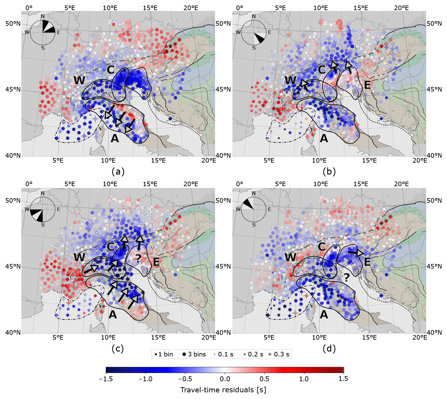
Figure 11 Travel-time residuals stacked for 90^∘ quadrants NE, SE, SW, NW. For each quadrant the travel-time average of three possible 30^∘ bins is shown. Circles of stations with incomplete coverage appear smaller; e.g. in (b) several directions are missing for OBS from SE direction, which has the lowest event coverage. Dashed lines show outlines of the same negative residual anomalies as in Fig. . Arrows indicate a lateral movement of anomaly imprints caused by an illumination of waves of different azimuths.

This fact is easily demonstrated for the four anomalies defined in the previous section. For example, for waves incident from the northeast (Fig. 10a), anomaly A is shifted to the southwest and can even be tracked by the OBS stations off the Italian coast. For waves incident from the southwest (Fig. 10c), it is shifted to the northeast and into the Adriatic Sea where we lose its track due to missing seismological stations. For waves arriving from perpendicular directions (Fig. 10b and d), it remains mostly in place.

Shifting and change of appearance is also observed for the anomalies C and E located between 12 and 15^∘ E. Both appear as strong, merging negative travel-time residuals for waves incident from NE (Fig. 10a) but seem to be weaker for waves arriving from other azimuths. For waves incident from SE (Fig. 10b) anomalies C and E appear to shift to the NW. The negative residuals of anomaly E almost completely disappear within the drawn outline. For illumination from the SW (Fig. 10c), anomaly C remains in place while, for illumination from the NW sector (Fig. 10d), anomaly C appears with a lower amplitude while anomaly E is shifted to the east.

The western Alpine anomaly (W) shows negative residuals for illumination from the SE that are shifted to the NW (Fig. 10b) but appears weak and partially positive for waves incident from the NW.

5.4 Frequency dependence

Owing to the high noise on the OBS records in the higher-frequency band, we assembled a low-frequency dataset with a maximum frequency of 0.1 Hz. As for the 0.5 Hz dataset, we determined absolute travel times and travel-time residuals using the same procedures as for the high-frequency data (including azimuthal binning, crustal corrections, etc.). We find that the obtained maps of travel-time residuals differ systematically between the considered frequencies (Fig. 11)

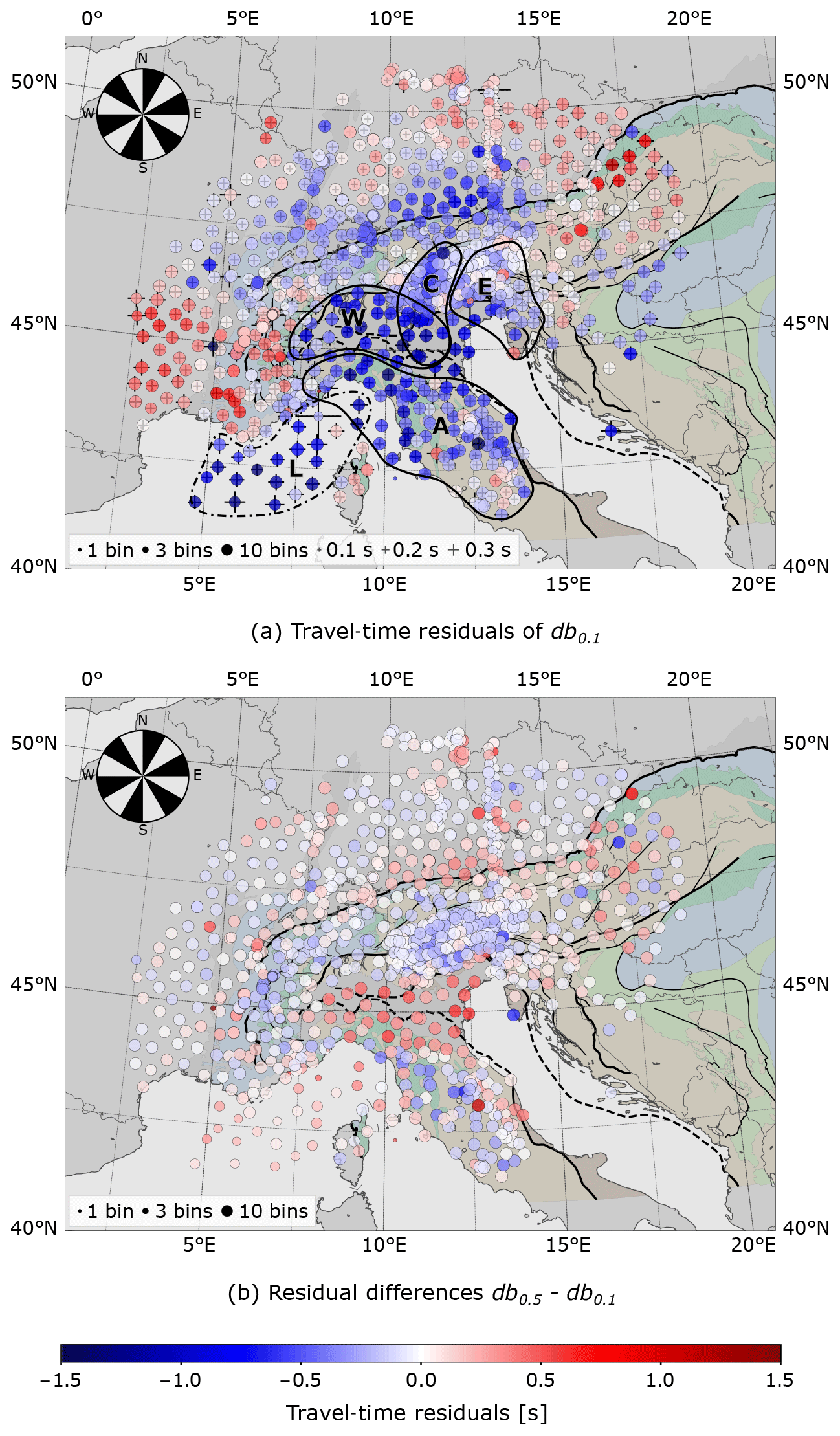
Figure 12 (a) Stacked travel-time residuals for 30^∘ bins from all directions for db_0.1 similar to Fig. . Patterns look similar in most areas to the one for the high-frequency dataset at first glance, except for weaker residual amplitudes. (b) Differences between stacked residuals of high- and low-frequency datasets show areas with positive sign (e.g. Po plain), or negative sign (e.g. Apennines, Alpine arc). Proportion of pick differences (same ray available in each dataset) to total number of picks in db_0.5 is 96 %.

To illustrate the differences between both frequency bands, we directly show travel-time residuals determined for the 0.1 Hz dataset (Fig. 11a), and we form differences of the travel-time residuals; i.e. we subtract the values for the low-frequency dataset from those of the high-frequency dataset (Fig. 11b).

There are no striking differences between residuals of db_0.5 (Fig. ) and db_0.1 (Fig. 11a), which in general show very similar patterns of negative and positive residuals. However, the negative residuals of the 0.1 Hz dataset seem smaller (up to 0.3 s) and less well-defined around the central (C) and eastern (E) anomalies. In contrast to that, there is a marked increase in amplitude of the negative residuals (up to 0.5 s) in the Po plain. In the remaining regions, deviations are rather small with a weak tendency to negative values, especially in the Alpine foreland.

There is a massive increase in the total number of picks for the ocean bottom seismometers reflecting the increase in onsets and onset quality described in Sect. 4. Also the variation of residuals with back-azimuth is lower for the OBS, because there are more picks available, even from the poorly covered back-azimuths. The number of OBS picks for all events increases from 421 to 1113 (+164 %), compared to a 25 % increase only for all stations. This might have a notable effect on resolving structures below the Ligurian Sea when performing a teleseismic tomography. In the case of the stacked travel-time residuals, no strong effect is visible because of the applied azimuthal binning.

6 Discussion

With large and dense arrays like AlpArray the amount of available records for travel-time measurements may readily accumulate to hundreds of thousands depending on the duration of the deployment. Hence, automatic procedures for determining travel times become mandatory. Moreover, with higher resolution capabilities of such arrays, demands on the accuracy of travel times have also increased, in particular if we want to resolve the correspondingly small travel-time differences between nearby stations. Sophisticated, automatic single-channel picking procedures apparently do not achieve the targeted accuracy for teleseismic travel times. To overcome this problem, measurements of relative time shifts between two traces by cross-correlation are used. They can be automated and are particularly well suited for dense arrays which provide a wealth of similar waveforms. However, they do not provide absolute travel times. For this reason, stacking or beamforming to obtain stable low-noise reference traces is an essential further element in travel-time determination (Rawlinson and Kennett, 2004). Mitterbauer et al. (2011) already used such an approach in their teleseismic tomography of the eastern Alps even though they only determined about 6600 travel times. They stacked records aligned to automatic picks to obtain low-noise reference traces for ensuing cross-correlation measurements. After determining cross-correlation time shifts they iterated the correlation and stacking step until a stable reference trace was obtained. Our approach is similar to that of Mitterbauer et al. (2011), as it also makes use of the elements automatic picking, beamforming and cross-correlation. But we found that iterative correlation and stacking were not necessary with AlpArray data, neither for the 0.5 nor the 0.1 Hz dataset. It proved to be sufficient to select one centrally located permanent station and correlate its waveform with the waveforms of all other stations to obtain time shifts for constructing a stable and very low noise reference or beam trace. Picking this beam trace automatically and using it as a reference trace for cross-correlation time-shift measurements was sufficient to obtain highly accurate relative and absolute travel times for up to 210 000 records in a fully automated fashion.

The uncertainty of a cross-correlation time delay measurement is evidently related to the width of the maximum of the cross-correlation function where the time delay is read off. We measure the full width at half-maximum (FHWM) which is, however, a too conservative estimate of the real error. For this reason, we include the maximum normalised correlation C_max as a second component into the error estimation. The higher the maximum correlation, the better is the delay time estimate. We account for this expectation by scaling the FHWM by a factor of $\mathrm{1}-C_{max}$. This definition reflects our expectation of higher uncertainties at lower frequencies because low-frequency waveforms tend to be smoother and onsets more emerging. In addition, it allows a consistent and automatic determination of uncertainty. Our reconstructions of smooth and nearly unperturbed wave fronts across the entire array from the observed travel-time field, with wave fronts separated by only 1 s of travel time demonstrate that the estimated travel-time uncertainties of on average 0.2 s (median 0.15 s) are realistic since otherwise conspicuous deformations should appear in the wave fronts, as they indeed do when the wave fronts are constructed from the automatic picks. Further evidence for the consistency and accuracy of the estimated travel times and travel-time residuals are the coherent and reproducible maps of travel-time residuals obtained for individual events, which correlate well with undulations of the reconstructed wave fronts.

We do not perform a tomographic inversion of the dataset here (which will be presented in a follow-up paper), but the maps of residual travel times and in particular their azimuthal variations already allow some inferences on the underlying mantle heterogeneities. We focus here on the maps of stacked residuals in Figs.  and 10 and the previously defined anomalies W, C, E and A to attempt some preliminary interpretations regarding mantle structures that might produce these anomalies.

Teleseismic waves can be considered as planar waves propagating through the subsurface and accumulating travel-time residuals on their way to the surface. Lags or advances of travel time due to velocity perturbations in the mantle are transported by the ray to the surface where they finally appear as travel-time residuals. The lateral shift between the location of the velocity perturbation and its associated travel-time residual at the surface depends on the incidence angle of the ray. This angle is not constant but, owing to the increase in seismic velocity with depth in the earth, decreases successively as the waves approach the surface. Thus, for velocity perturbations at shallow mantle depths and hence subvertical rays we expect small lateral shifts while we expect large lateral shifts for deep seated perturbations. On top of that, variations of the location of travel-time residuals with azimuth allow some inferences on the dip of a velocity perturbation. For example, a dipping slab will produce a maximum travel-time residual for teleseismic waves entering it along the updip direction.

Based on these considerations, we conclude that travel-time residuals that stack coherently over all azimuths must be caused by velocity perturbations located in the shallow mantle. Thus, the anomalies W, C, E and A appearing in the overall stack in Fig.  hint at fast shallow mantle probably associated with the lithospheric slabs below the western, central and eastern Alps and the Apennines. In particular, the strike of anomaly A correlates well with the strike of the Apenninic mountain chain, forming a narrow band along the western Italian coast in the north and then opening up into a broad band below central Italy. The large lateral shift of anomaly A with azimuth (Fig. 10) indicates that the Adriatic slab below the Apennines extends deep into the upper mantle. The same applies to anomaly E, associated with the eastern Alpine slab, which also exhibits a considerable lateral shift depending on azimuth. Lateral shifts of anomalies C and W are not that strong, implying that the central and western Alpine slabs terminate at shallower depths compared to the Adriatic slab below the Apennines and eastern Alpine ones. The fact that anomalies C and E appear strongest for waves arriving from the NE hint at a NE-ward dip of the associated slabs. However, since variation with azimuth of anomaly C is weaker than that of anomaly E, the central Alpine slab is inferred to dip more steeply than the eastern one. In contrast, the Apennine slab seems to be close to vertical as the amplitude of anomaly A is rather independent of azimuth. Anomaly W appears strongest for waves incident from SE and weakest for waves arriving from NW. This indicates a SE dip of the western Alpine slab. Finally, the stable positive anomalies under the Ligurian sea are interpreted as thin oceanic crust underlain by shallow fast upper mantle.

Besides the areas of negative travel-time residuals, we find large regions of positive residuals in SE France and in the northeastern corner of AlpArray. These anomalies appear in the overall stack of the residuals (Fig. ) and only show a weak variation with wave azimuth (Fig. 10), indicating a slow lithospheric and asthenospheric mantle beneath these areas potentially due to a delamination of former mantle lithosphere (in the NE) or upwelling of asthenospheric material beneath SE France.

The fact that the negative anomalies along the Alpine chain in Fig.  are separated by regions of zero to weakly negative residuals indicates a segmentation of the slabs beneath the Alps. Transitions occur at about 10^∘ E close to the boundary between the western and eastern Alps and at 12^∘ E at the western rim of the Tauern window. This laterally discontinuous behaviour of the travel-time residuals matches previous findings by Lippitsch et al. (2003) and Mitterbauer et al. (2011), who identified different lateral slab segments in the western, central and eastern Alps with possible changes in slab dip. In particular, the slab structure belonging to anomaly E is disputed because Lippitsch et al. (2003) favour a north-dipping slab while Mitterbauer et al. (2011) infer a nearly vertical slab. Unfortunately, it is hardly possible to infer more quantitative details on mantle structure from the stacked travel-time residuals only because they integrate over depth. This problem can only be overcome by a tomographic inversion of the event-specific maps of travel-time residuals. Nevertheless, the preliminary guesses on mantle structure may serve as qualitative plausibility constraints for a later tomography.

Another interesting aspect of our travel-time measurements is their frequency dependence, in particular the differences between the travel-time residuals derived from the 0.5 and the 0.1 Hz dataset. Physical reasons for a frequency dependence of travel-time residuals estimated by cross-correlation can be dispersion due to attenuation (Liu et al., 1976) or the fact that the interaction of seismic waves with heterogeneous structures depends on wavelength and hence also on frequency. The former describes the fact that the velocity of waves in attenuating media becomes frequency dependent while the latter leads to deviations from predictions of ray theory which is a zero-wavelength approximation. It is often referred to as the finite-frequency effect with wave front healing (Wielandt, 1987) as one prominent example. One may also suspect that the applied low-pass filter may affect the travel-time residuals as the group delay of the filter increases with decreasing corner frequency. However, assuming that all travel times at the lower-frequency f₁ are delayed relative to those at the higher-frequency f₂ by Δτ implies that the array averages are also delayed by Δτ. Since we subtract the array average the delay cancels, making the demeaned residual filter independent. Thus, frequency dependence of the travel-time residuals should be explained by the physical reasons mentioned above.

We argue here that the frequency dependence is due to the finite-frequency effect because dispersion due to attenuation predicts disparity patterns which are inconsistent with the observations. The negative differences between the travel-time residuals of the 0.5 and the 0.1 Hz dataset in the region of anomalies C and E as well as the positive ones in the area of the Po plain (Fig. 11b) can be plausibly explained by the fact that low-frequency waves (0.1 Hz) and their travel times are less influenced by both high-velocity anomalies beneath C and E and the low P wave velocity sediments that are only few kilometres thick in the Po plain than the high-frequency waves at 0.5 Hz. Thus, residuals at 0.1 Hz are less negative than at 0.5 Hz for high-velocity heterogeneities, leading to a negative difference, and less positive than at 0.5 Hz for low-velocity heterogeneities, leading to a positive difference. This effect leads to an overestimation of negative residuals in the Po plain after crustal correction for the 0.1 Hz dataset, as our simple crustal correction approach does not account for the finite-frequency effect. On the contrary, dispersion due to attenuation would produce a very different effect. According to Liu et al. (1976), high-frequency waves should travel increasingly faster compared to low-frequency ones with increasing attenuation. Thus, over regions of high velocities with potentially low attenuation frequency disparity should be close to zero. Moreover, over low-velocity regions with potentially high attenuation we would expect a negative frequency disparity. Both tendencies are opposite to what we observe.

7 Conclusions

The dense AlpArray Seismic Network and its complementary deployments offer the unique opportunity to infer mantle structure beneath the greater Alpine region with an unprecedented resolution. However, to benefit fully from the array, absolute travel times and travel-time residuals of high accuracy and consistency are required. We have shown that even very sophisticated automatic picking algorithms based on higher-order statistics and the Akaike information criterion is unable to fulfill this requirement. We demonstrate that, instead, a hybrid approach combining characteristic function picking, waveform cross-correlation and beamforming techniques that takes advantage of the dense array is indeed capable of achieving the required accuracy. Since this hybrid approach is also fully automated, human effort is drastically reduced and the consistency of the generated dataset is ensured by the reproducibility of the automatically determined onsets. Beamforming requires similar waveforms posing demands on array density depending on frequency range. The AlpArray seismic network proved to be sufficiently dense to obtain high waveform correlation at the chosen low-pass-filter frequencies (0.5 and 0.1 Hz). Admitting higher frequencies may require smaller interstation distances to preserve waveform coherency.

The accuracy of travel times and residuals is validated by the fact that they allow a reliable and flawless construction of teleseismic wave fronts in terms of travel-time isochrons. These exhibit small undulations indicating the presence of mantle heterogeneities. The travel-time residuals for individual events show very coherent and reproducible spatial patterns that perfectly fit to these undulations and, although masked by their dependence on illumination incidence and azimuth, already give a glimpse into mantle velocity anomalies, in particular conspicuous slab-like high-velocity structures along the Alpine arc and the Apennines. Studying the azimuthal variations of the residuals provides the first hints of the dip of these anomalies. Even stacks of residuals maps from hundreds of events show distinct, spatially coherent areas of positive and negative residuals and, in particular, reproduce the conspicuous negative residuals. These results indicate the stable presence of mantle heterogeneities in each map of travel-time residuals and allow us to make assertions about the geometry and position of the high- and low-velocity objects below the Alps even before performing a full teleseismic tomography.

Maps of travel-time residuals derived from data filtered to different maximum frequencies show similar patterns but are different with respect to amplitude and sharpness of the anomalies confirming that the sensitivity of waves to heterogeneities depends on wavelength. Hence, datasets of travel time and residuals obtained from differently filtered waveforms cannot be used together in a classical travel-time tomography.

Appendix A

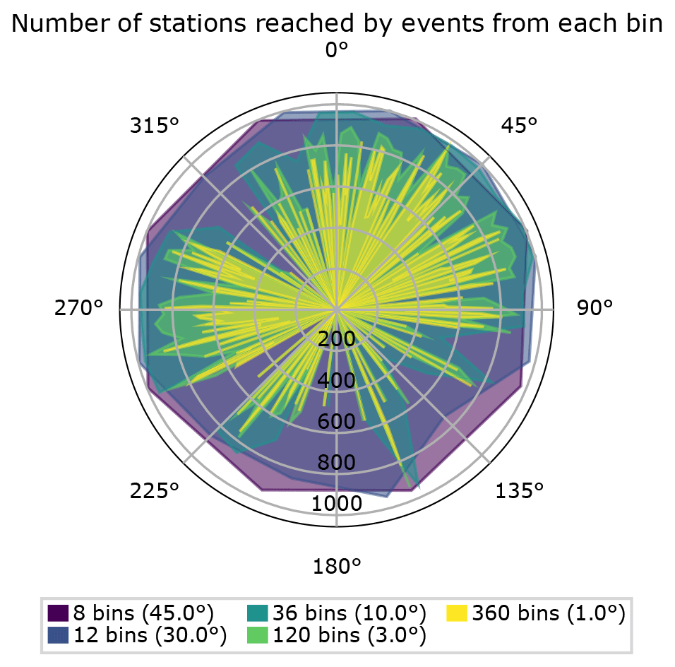
Figure A1 Number of stations for each bin for different bin sizes. Distribution is rather homogeneous for 30 and 45^∘ bins. With smaller bin sizes bias increases, which downweights back-azimuths with low event coverage.

Figure A2 Vertically stacked travel-time residuals of crustal model compared to reference minimum 1D model of D09a, showing the potential crustal contributions on teleseismic travel-time residuals. The most prominent features are the high-velocity anomaly in the western Alps (Ivrea body) and the low-velocity anomaly of the Po plain. Low velocities of Molasse sediments are compensated by higher velocities in the crust of the Diehl model.