the Creative Commons Attribution 4.0 License.
the Creative Commons Attribution 4.0 License.
 | 25 Nov 2021
Imaging structure and geometry of slabs in the greater Alpine area – a P-wave travel-time tomography using AlpArray Seismic Network data
Wolfgang Friederich
Stefan M. Schmid
Mark R. Handy
We perform a teleseismic P-wave travel-time tomography to examine the geometry and structure of subducted lithosphere in the upper mantle beneath the Alpine orogen. The tomography is based on waveforms recorded at over 600 temporary and permanent broadband stations of the dense AlpArray Seismic Network deployed by 24 different European institutions in the greater Alpine region, reaching from the Massif Central to the Pannonian Basin and from the Po Plain to the river Main.
Teleseismic travel times and travel-time residuals of direct teleseismic P waves from 331 teleseismic events of magnitude 5.5 and higher recorded between 2015 and 2019 by the AlpArray Seismic Network are extracted from the recorded waveforms using a combination of automatic picking, beamforming and cross-correlation. The resulting database contains over 162 000 highly accurate absolute P-wave travel times and travel-time residuals.
For tomographic inversion, we define a model domain encompassing the entire Alpine region down to a depth of 600 km. Predictions of travel times are computed in a hybrid way applying a fast TauP method outside the model domain and continuing the wave fronts into the model domain using a fast marching method. We iteratively invert demeaned travel-time residuals for P-wave velocities in the model domain using a regular discretization with an average lateral spacing of about 25 km and a vertical spacing of 15 km. The inversion is regularized towards an initial model constructed from a 3D a priori model of the crust and uppermost mantle and a 1D standard earth model beneath.
The resulting model provides a detailed image of slab configuration beneath the Alpine and Apenninic orogens. Major features are a partly overturned Adriatic slab beneath the Apennines reaching down to 400 km depth still attached in its northern part to the crust but exhibiting detachment towards the southeast. A fast anomaly beneath the western Alps indicates a short western Alpine slab whose easternmost end is located at about 100 km depth beneath the Penninic front.
Further to the east and following the arcuate shape of the western Periadriatic Fault System, a deep-reaching coherent fast anomaly with complex internal structure generally dipping to the SE down to about 400 km suggests a slab of European origin limited to the east by the Giudicarie fault in the upper 200 km but extending beyond this fault at greater depths. In its eastern part it is detached from overlying lithosphere. Further to the east, well-separated in the upper 200 km from the slab beneath the central Alps but merging with it below, another deep-reaching, nearly vertically dipping high-velocity anomaly suggests the existence of a slab beneath the eastern Alps of presumably the same origin which is completely detached from the orogenic root.
Our image of this slab does not require a polarity switch because of its nearly vertical dip and full detachment from the overlying lithosphere. Fast anomalies beneath the Dinarides are weak and concentrated to the northernmost part and shallow depths.
Low-velocity regions surrounding the fast anomalies beneath the Alps to the west and northwest follow the same dipping trend as the overlying fast ones, indicating a kinematically coherent thick subducting lithosphere in this region. Alternatively, these regions may signify the presence of seismic anisotropy with a horizontal fast axis parallel to the Alpine belt due to asthenospheric flow around the Alpine slabs. In contrast, low-velocity anomalies to the east suggest asthenospheric upwelling presumably driven by retreat of the Carpathian slab and extrusion of eastern Alpine lithosphere towards the east while low velocities to the south are presumably evidence of asthenospheric upwelling and mantle hydration due to their position above the European slab.
- Article
(48449 KB) - Full-text XML
- Companion paper 1
- Companion paper 2
-
Supplement
(4280 KB) - BibTeX
- EndNote


For well over a century, the Alps have been the breeding ground for revolutionary ideas in geodynamics that serve as blueprints for understanding other major orogens in the world. The Alps exhibit the entire spectrum of orogenic processes, from juvenile stages in their eastern part to mature stages in the central and western regions. They are marked by highly dynamic small-scale interactions of microplates in a setting of Europe–Africa convergence which produced their unique arcuate, non-cylindrical shape and lead to characteristic along-strike changes of structure. In spite of their small size, they exhibit significant topographic relief. Several regions in the Alps (e.g. Friaul) are prone to considerable seismic hazard and, owing to the high population density, suffer from high vulnerability to natural disasters.

Figure 1Tectonic map of the Alpine chains compiled by M. R. Handy showing different seismic networks as well as temporary experiments, tectonic units and major fault systems.
Due to these unique characteristics, the Alps have been the subject of continuous seismological research. Crustal structure was intensively studied using active seismic refraction and reflection surveys (e.g. Blundell et al., 1992; Mueller and Banda, 1983; Hirn et al., 1989; Pfiffner et al., 1988; Frei et al., 1989; TRANSALP Working Group et al., 2002). On top of that, crustal velocities and Moho topography were investigated using local earthquake tomography (e.g. Diehl et al., 2009), receiver functions (e.g. Lombardi et al., 2008; Kummerow et al., 2004) and ambient noise tomography (e.g. Stehly et al., 2009; Fry et al., 2010; Molinari et al., 2015). Models of mantle P-wave velocity structure were derived from teleseismic body wave tomography both on regional scale (Babuška et al., 1990; Lippitsch et al., 2003; Mitterbauer et al., 2011; Karousova et al., 2013; Zhao et al., 2016) and continental scale (e.g. Spakman et al., 1993; Piromallo and Morelli, 2003). First concepts of mantle flow beneath the western Alps were developed from results of shear-wave splitting analysis (Barruol et al., 2011) while topography of the mantle discontinuities was mapped using receiver functions (Lombardi et al., 2009). Continental-scale models of mantle S-wave velocities were inferred from surface waves either by inversion of waveforms (Marone et al., 2004; Legendre et al., 2012) or dispersion curves (Peter et al., 2008; Boschi et al., 2009; El-Sharkawy et al., 2020), from S-wave travel times (Schmid et al., 2008) and from adjoint full waveform inversion (Zhu et al., 2012). Recently, Kästle et al. (2018) derived a regional-scale S-wave model of the greater Alpine region by combining surface wave dispersion extracted from earthquake and ambient noise data.
The current picture of the deep structure of the Alps that can be drawn from the seismological results looks as follows: the crust is characterized by stacking and wedging of tectonic units of European and Adriatic provenience to accommodate crustal shortening during collision. The Moho is discontinuous with gaps as well as vertical offsets between the European and the Adriatic Moho (e.g. Spada et al., 2013). The mantle below is pervaded by distorted, corrugated and torn slab segments of presumably continental origin whose dip apparently flips from SE in the western to central parts to NE in the eastern part of the Alps. This postulated polarity flip is a unique feature of Alpine orogeny and has not been observed elsewhere in the world. Further east, in the northern Dinarides, a slab seems to be entirely missing. Deep in the transition zone, the entire Alpine belt and the southern forelands are underlain by seismically fast material interpreted as remnants of the Alpine Tethys subducted during the Late Cretaceous to Early Paleogene (Handy et al., 2010).
Despite the successes of Alpine geophysical research, the current state of knowledge on the deep structure of the Alps cannot be considered as satisfactory given major open questions and new opportunities of seismological observation and imaging. A clear definition of the structural properties of the lithosphere is still lacking. How do slabs behave in the shallower regions? What is the nature of coupling of the slabs with the plates at the surface? How does it influence surface topography? Are parts of the subducted slabs still attached to the plate? Which parts (lower crust, lithospheric mantle) have sunk into the mantle? Images of oppositely dipping slab segments as well as their interpretation are still controversial. Is European or Adriatic lithosphere subducted in the eastern Alps?
The internal structure, outer boundaries and provenance of subducted material are poorly constrained. Suggested slab tears in the western and central Alps (Lippitsch et al., 2003; Kästle et al., 2020) remain enigmatic. Up to now, resolution is concentrated on the core region of the Alps; hence extensions as well as connections of subducted material to surrounding lithosphere and asthenosphere are unclear. What role did the old Variscan basement play during Alpine orogeny? To what extent is lithospheric structure inherited from this older history? Finally, how thick and how long are the descending slabs? Where are the younger slabs connected to the older subducted material stacked in the transition zone? How much subducted material has accumulated in the transition zone? Answering these questions is essential for plate tectonic reconstructions and geodynamic modelling.
In this paper, we attempt to provide answers to most of the questions formulated above by means of a teleseismic tomography of the mantle beneath the Alpine mountain belt and neighbouring parts of the Apennines, Dinarides and their forelands. The observational basis for this study is the AlpArray Seismic Network (AASN, Hetényi et al., 2018), the complementary experiments EASI (Eastern Alpine Seismic Investigation, EASI, 2014) and Swath-D (Heit et al., 2017) dedicated to specific target regions in the Alps, and a joint German–French ocean bottom seismometer deployment in the Ligurian sea (LOBSTER and ALP-ARRAY-FR). The AASN covers the entire Alpine mountain belt including the forelands from the Massif Central in the west to the Pannonian Basin in the east, and from the river Main in Germany in the north to the Po river in the south. In its full configuration, it encompassed about 600 seismic broadband stations (Fig. 1).
Compared to the stations available for previous body wave tomographic images (Lippitsch et al., 2003; Koulakov et al., 2009; Mitterbauer et al., 2011; Zhao et al., 2016), which form the basis for our current view of the mantle beneath the Alps, the AASN constitutes a massive improvement of observational coverage by filling gaps between the stations of the permanent networks with additional temporary ones. The total number of onsets used in this study exceeds the number of measured onsets by Mitterbauer et al. (2011) by a factor of 24 and those of Lippitsch et al. (2003) by a factor of 38. The AASN is the densest seismic network ever to cover an entire mountain belt and permits unprecedented images of the 3D distribution of seismic velocities in the lithosphere and the sub-lithospheric mantle.
In Sect. 2, we sketch the methods applied to extract travel times and travel-time residuals from the original waveform data and to make predictions of travel times for teleseismic P-wave phases. Moreover, we describe the inversion procedure and our approach of implementing the effect of crustal structure into the inversion procedure. Section 3 describes the data basis of this study in a brief manner as a detailed analysis of the travel-time data is already provided by Paffrath et al. (2021a). Section 4 gives an analysis of resolution by means of checkerboard tests, and in Sect. 5 we present the tomographic velocity model based on horizontal and selected vertical cross sections. The discussion in Sect. 6 gives an interpretation of the structural significance of the observed velocity anomalies, in particular focusing on the geometry of subducted lithosphere beneath the Alps. Our results are compared to previous tomographies by Lippitsch et al. (2003), Mitterbauer et al. (2011), Koulakov et al. (2009) and Zhao et al. (2016). We conclude with a 3D image of the slab configuration beneath the Alps directly derived from the tomographic model.
2.1 Measuring travel times and travel-time residuals
We define here travel time τj as the difference between the measured arrival time of the P wave at some station j and the origin time of the considered earthquake. For the latter, we use the centroid time given in the global CMT catalogue (Dziewonski et al., 1981; Ekström et al., 2012).
The process of determining travel times is described in detail by Paffrath et al. (2021a). A specially designed combination of automatic picking, waveform cross-correlation and beamforming is applied to attain the accuracy necessary for performing teleseismic tomography. Initial automatic picks based on higher-order statistics and the Akaike information criterion (Küperkoch et al., 2010) are used as anchor points for a first-stage cross-correlation with an appropriately selected reference station. Traces are then aligned to the reference trace and stacked to form a very low noise beam trace. The beam trace serves as reference trace for a second cross-correlation step in which time differences ΔτjB between the beam and the individual stations are measured. Absolute travel time τj is determined by automatically picking the beam trace, τB, and adding the time difference with respect to the beam:
In the teleseismic inversion described below, we do not use these absolute travel times but instead invert event-wise demeaned travel-time residuals for velocity perturbations. Demeaning is done to avoid errors of origin times and to reduce influences from remote earth structure not included in the inversion domain. Residuals are obtained by subtracting theoretical travel times of an appropriate 1D reference earth model from the observed travel times. Thus, the demeaned travel-time residual can be written as follows:
where denotes the observed travel-time array average, Tj the reference earth travel times and their array average. Inserting Eq. (1), we find
where denotes the array average of the time difference between station traces and beam.
Remarkably, the demeaned residual travel times can be calculated from the measured time differences between station trace and beam alone, and hence, their uncertainty is controlled by the uncertainty of these time differences. We estimate this uncertainty on the basis of the full width of the cross-correlation function at half-maximum, FWHM, and its normalized maximum value Cmax,jB:
This results in an uncertainty which tends to become larger with decreasing waveform frequency since cross-correlation maxima become wider. Moreover, waveforms deviating from the beam trace due to noise or additional complexity receive a larger uncertainty owing to a reduced maximum correlation.
2.2 Computation of synthetic travel times
Teleseismic tomography requires the computation of synthetic travel times for comparison with the observed ones. We compute travel times in a hybrid way using a fast method for the path from the source location to the inversion domain assumed to lie within a 1D standard earth model and a 3D eikonal solver for tracing the wave front through the inversion domain. Since the seismic velocity only changes in the inversion domain, rays and travel times through the standard earth model are only computed once for each event whereas travel times in the inversion domain are recalculated in each iteration of the inversion. We use the TauP routine (Crotwell et al., 1999) implemented in ObsPy (Krischer et al., 2015) to calculate ray propagation in the global earth. The ray parameters and travel times are saved on each boundary surface exposed to the source. From there, the incident wave front is continued into the three-dimensional model using the FM3D algorithm by Rawlinson and Sambridge (2005).
The influence of global heterogeneities on rays between a given source and the array is expected to be low, as rays are bundled for the largest part of the travel path and only spread into different directions when approaching the inversion domain. Thus, the influence of remote heterogeneities will mostly affect all rays from a given source in the same way and is eliminated when subtracting the array average. Moreover, we assume the earth's lower mantle to be weakly heterogeneous in P-wave velocity (e.g. Aki et al., 1977) in contrast to the upper mantle and crust below the Alps. However, there will be remaining influences of the earth's lower mantle on our model.
2.3 Inversion method
The inverse problem is solved using the inversion scheme implemented in FMTOMO (Rawlinson et al., 2006). Demeaned travel-time residuals as defined in Eq. (2) are inverted for P-wave velocity, minimizing the objective functional:
with m denoting the 3D P-wave velocity model, m0 the initial P-wave velocity model, g(m) predicted mean-corrected residuals, dobs observed demeaned residuals and Cd an a priori data covariance matrix representing the uncertainties of the residuals. The first term represents the misfit between observations and predictions while the two following terms define the squared model norm which is a measure of the complexity of the model. The first term of the model norm describes the variance of the model with respect to the initial model scaled by a priori variances contained in the matrix while the second term quantifies the roughness of the model using the matrix D which implements a 3D Laplacian differential operator. The relative weight of variance, roughness and misfit in the objective function can be controlled by the parameters ϵ and η. Misfit and model norm play against each other: reducing the misfit implies increasing the model norm and vice versa. The aim of the inversion is to find a model that reduces the misfit to a certain threshold and minimizes the model norm.
Variance and roughness parameters are selected with the help of synthetic tests, where we investigate the recovery of a known input model after a fixed number of iterations and with the help of trade-off curves by which we try to balance out misfit and model norm. We will show such a curve in Fig. 11 when analysing the actual trade-off for different variance and roughness parameters in Sect. 5. The ideal trade-off is found on the curve somewhere close to the maximum curvature.
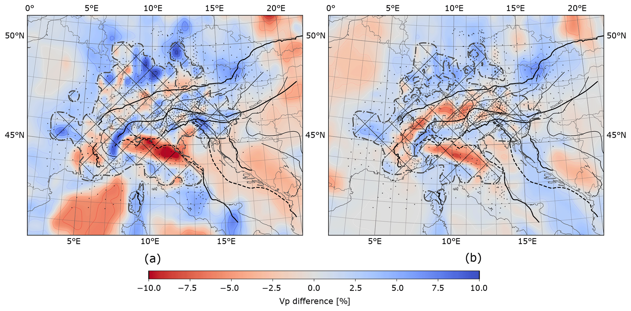
Figure 2Two horizontal slices through the (smoothed) crustal model at (a) 15 km and (b) 30 km depth. Colours show the difference in P-wave velocity to the one-dimensional background model. Dashed–dotted line indicates boundary between the two models of Diehl et al. (2009) (cross-hatched area) and Tesauro et al. (2008).
The inverse problem is non-linear because the forward problem g(m) is a non-linear functional. For this reason, the minimum of the objective functional is searched iteratively. In each iteration, the linearized inverse problem is solved using a sub-space projection method and the predicted travel times g(m) are updated using the fast-marching method (Rawlinson and Sambridge, 2005). Iterations are stopped if the misfit over number of data defined by
either reaches 1, signifying that the data are fit down to their uncertainties, or if misfit reduction stagnates when executing further iterations.
The model is discretized by defining the model parameters m as the values of P-wave velocity on a regular grid with a spacing of 0.23° in latitude, 0.3° in longitude and 15 km in depth. This corresponds to a lateral grid spacing of about 25 km. The bounds of the model domain are at 31 and 61° in latitude, −13 and 35° in longitude, and a depth of 600 km. Surface topography is taken into account implicitly by correctly positioning the receivers into the model grid. The centre of the inversion domain is at 46° latitude and 11° longitude. The total number of grid points and thus model parameters is 884 520. The lateral dimensions of the computational box were chosen to be larger than actually necessary for the inversion. Due to numerical errors of up to 0.3 s in the synthetic travel times near the lateral boundaries of the model domain when calculated with the hybrid method, we have increased the model domain to ensure that travel-time errors in the relevant areas of the model stay below 0.01 s. For consistency, we also used the hybrid method for the calculation of the teleseismic reference travel times.
2.4 Integration of a priori high-resolution models of the crust and uppermost mantle
The observed travel-time residuals contain contributions from mantle and crustal heterogeneities. Unfortunately, resolution of crustal structures by teleseismic waves is very limited. Owing to the sub-vertical propagation of teleseismic waves through the crust, crossing of rays is essentially inhibited leading to a complete loss of vertical resolution. Hence, to infer mantle structure, an a priori velocity model of the crust based on independent data is required (e.g. Kissling, 1993).
While the standard approach is either a direct correction of the observed travel-time residuals at each station assuming vertical wave propagation through the crust (e.g. Zhao et al., 2016), or an event-wise calculation of crustal residuals (e.g. Lippitsch et al., 2003), we directly integrate the external crustal model into the velocity model of our teleseismic inversion. In this way, ray refraction in the crust depending on vertical and azimuthal incidence is correctly treated. Moreover, we may use the variance term of the model norm to assign spatially varying variances to velocities in the crustal region that reflect the reliability of the external crustal model. This allows the inversion to deviate from the a priori crustal velocities if required by the teleseismic data. Finally, with this method, we obtain a velocity model covering crust and mantle that consistently reconciles imported crustal heterogeneities and teleseismic data.
We have assembled a new P-wave velocity model of the crust and uppermost mantle beneath the greater Alpine region (Fig. 2) mainly based on the model EuCRUST-07 by Tesauro et al. (2008) and the fully three-dimensional, high-resolution P-wave velocity model of the central Alpine crust provided to us by Diehl et al. (2009). EuCRUST-07 is discretized laterally on a 15′ times 15′ regular grid. Vertically, each grid cell contains three layers composed of sediments and upper and lower crust. Values of thickness and seismic velocities are specified for the crustal layers while only thickness is given for the sediment layer. Here, we use a constant value of 2.8 km/s for the P-wave velocity of the sediments. EuCRUST-07 was compiled from results of various seismic reflection, refraction and receiver function studies. The model by Diehl et al. (2009) was derived using local earthquake tomography and provides the most precise information on crustal (and uppermost mantle) velocity structure. However, it only covers about two-thirds of the lateral dimensions of AlpArray and has varying resolution that reflects the available distribution of local earthquakes and seismic stations. For simplicity, we hereinafter also refer to the model resulting from this study as Diehl's model. Furthermore, we take advantage of a more recent study of Spada et al. (2013), which focuses on the greater Alpine area, to update Moho depth and hence crustal thickness of the EuCRUST-07 model.
To construct the a priori crustal model, we discretized the modified EuCRUST-07 model on a regular km grid. In the regions where Diehl's model provides P-wave velocity values, we form a linear combination of both models with weights reflecting the reliability of Diehl's model. The weights are calculated on the basis of the diagonal elements of the resolution matrix (RDE) provided to us by T. Diehl (personal communication, 2020). The weight is calculated with a transfer function (Fig. 3), favouring the sufficiently well resolved parts of the model of Diehl et al. (2009) over that of Tesauro et al. (2008). Finally, since the discretization of the inversion domain is much coarser than the km grid, we resample the velocity values of our a priori model using a 3D Gaussian kernel as a spatial filter to prevent aliasing effects. Because Diehl's velocity model also contains valuable information about the uppermost mantle the resulting a priori model is strictly speaking not solely a crustal model. For the sake of simplicity; however, we will refer to it from here on as the a priori crustal model.
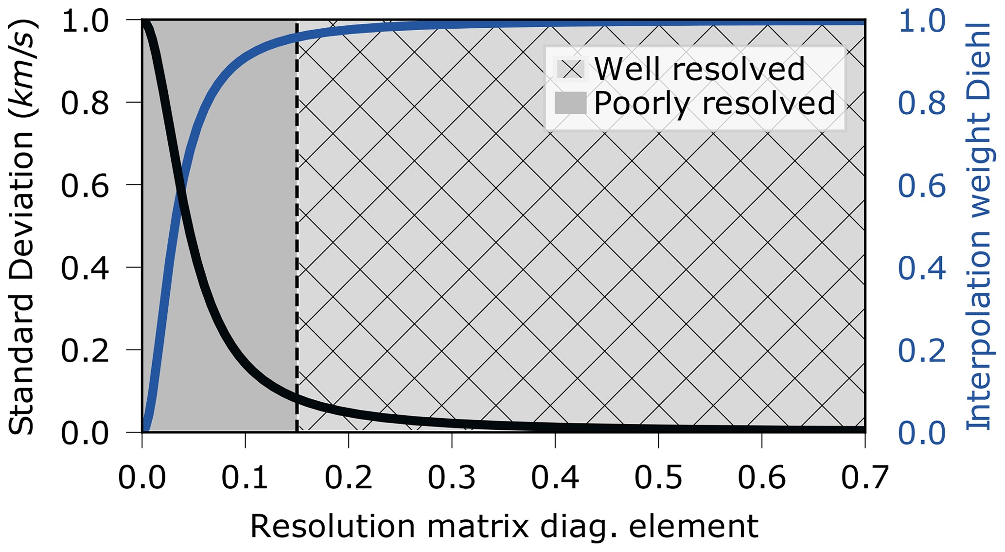
Figure 3Black line: transfer function mapping RDE values provided by Diehl to a priori standard deviations of P-wave velocity. Blue line: transfer function mapping RDE values to interpolation weights for Diehl's model.
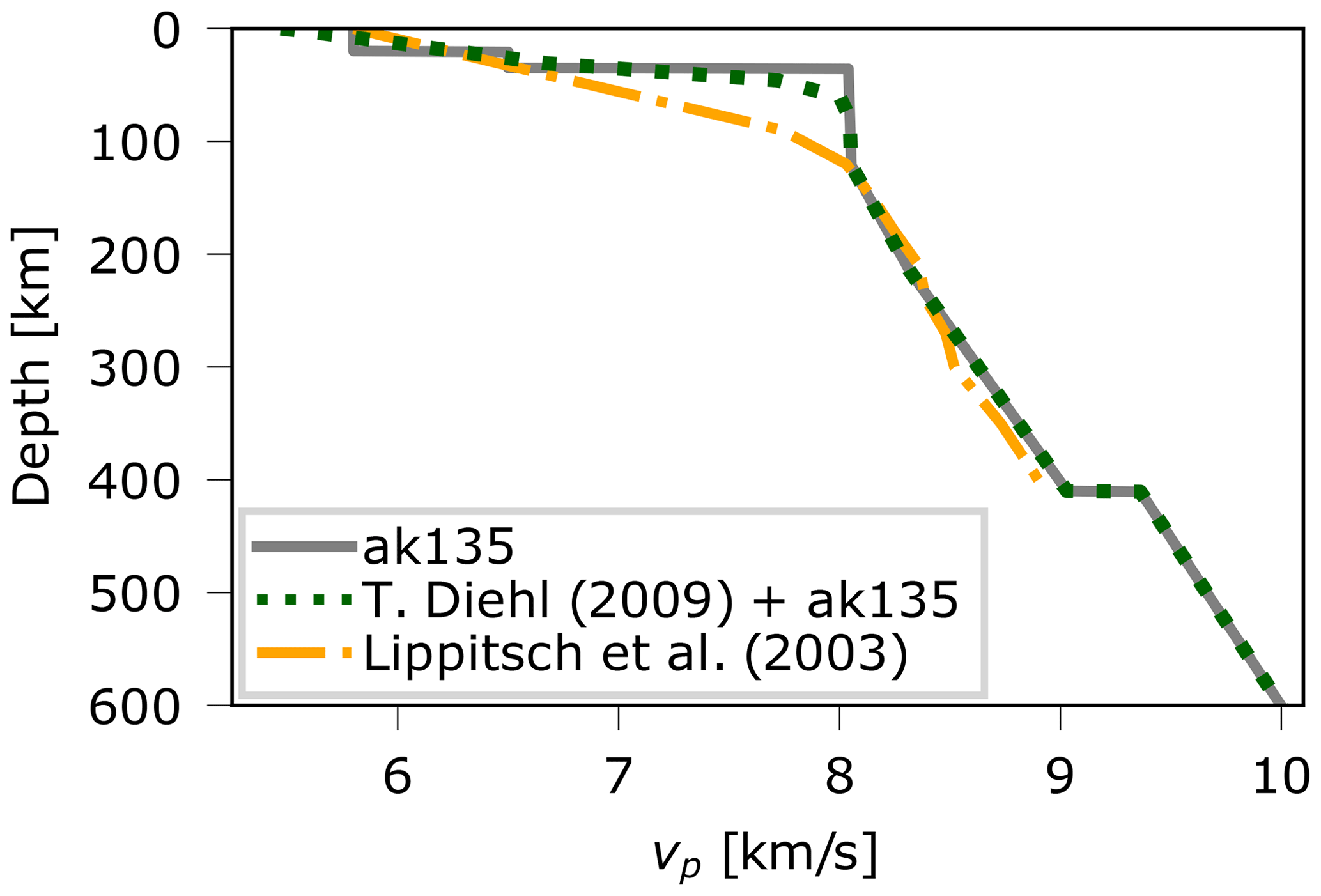
Figure 4Dotted line: one-dimensional model used in this study as initial model for the inversion in regions beyond the extent of the a priori crustal model. For comparison, the standard earth model AK135 (solid line) and the reference model used by Lippitsch et al. (2003) (dashed–dotted line).
The 3D a priori crustal model is incorporated into the initial model for the inversion. A detailed description of this process can be found in the Appendix. For the regions of the inversion domain beyond the extent of the a priori crustal model, we assume a modified standard earth model (dotted line in Fig. 4) constructed from the standard earth model AK135 (Kennett et al., 1995) and the 1D reference model used by Diehl et al. (2009). The transition from the a priori crustal model to this model occurs at a depth of 77.5 km.
We also estimate a priori standard deviations for different parts of the crustal model which control the amount of adjustments of P-wave velocity allowed during teleseismic inversion. For regions in our crustal model controlled by the model of Diehl et al. (2009), we use again an empirical transfer function to calculate a standard deviation for a given RDE value (Fig. 3). In the remaining regions, where we use the model of Tesauro et al. (2008), we assume an equivalent RDE of 0.1 for the sedimentary basins and the lower crust and 0.15 for the upper crust corresponding to a standard deviation of 0.17 and 0.082 km/s, respectively. It should be noted here that the effect of our a priori crustal model on the inversion result is additionally influenced by the damping parameter ϵ. For this reason, it is rather the ratios of the standard deviations than their absolute values that matter.
As already mentioned, this study is founded on data from the AlpArray Seismic Network (AASN, Hetényi et al., 2018), the complementary experiments EASI (Eastern Alpine Seismic Investigation, EASI, 2014) and Swath-D (Heit et al., 2017), and a joint German–French ocean bottom seismometer deployment in the Ligurian sea (LOBSTER and ALP-ARRAY-FR). In its full extent, the network encompassed about 600 seismic broadband stations of which about one-half are permanently operating stations and the other half temporarily deployed stations (Fig. 1).
Installation of stations began in July 2015 mainly in Austria and northern Italy, followed by stations covering southern Germany in November–December 2015 and eastern France in summer 2016. Ocean bottom seismometers were deployed from June 2017 to February 2018. The earliest complementary experiment, partly included in our dataset, is the EASI project with 55 stations deployed on a north–south profile at 13.4° E traversing the Alps from the northern Alpine foreland to the Adriatic Sea and recording ground motion for more than a year until August 2015. The second complementary experiment, Swath-D, running for 2 years from the end of 2017 and covering a broad swath across the eastern Alps including the Tauern window, further improved station density in a key area of the Alps.
To further extend the station coverage to the north and south, we include all permanent and temporary stations available at the time of request in the greater Alpine region, within a 5° radius around 46° N and 11° E, i.e. mainly stations in central Germany and northern Italy, in our dataset. With that we finally assemble waveforms from a total of 1025 different seismic broadband stations with recording times scattered through a period of over 4.5 years between 2015 and the end of 2019, with a peak in station coverage of more than 720 stations in late 2017.
We give here only a brief overview of the travel-time database that was extracted from the recorded waveforms. For more detailed information, we refer the reader to Paffrath et al. (2021a), who provide an in-depth analysis of the measured travel times and travel-time residuals and their errors. In that study, travel times were measured on waveforms filtered with a Butterworth bandpass filter with a lower corner frequency of 0.03 Hz and an upper corner frequency of 0.1 and 0.5 Hz, respectively. For the present study, we invert travel-time residuals obtained from the higher-frequency waveforms filtered to 0.5 Hz because they exhibit smaller uncertainties and thus higher spatial resolution. The resulting database comprises 162 366 travel times of 331 events of magnitude 5.5 or higher.
Suitable events were carefully selected first on a single-station basis, i.e. by setting a minimum cross-correlation coefficient value with regard to the beam trace of 0.6. Moreover, wave fronts were constructed for each event and large outliers (with respect to an average planar wave front) were automatically removed. In addition, each wave front was visually inspected to check for suspicious bumps that could be attributed to false onsets on a single station. We found only a few of these outliers, which could be attributed to possible GPS timing errors at the respective stations. We also visually inspected the travel-time residual patterns of all events to ensure smooth variation with back-azimuth and epicentral distance. Finally, a threshold of at least 100 onsets per event was used to guarantee an even distribution of onsets across the array.
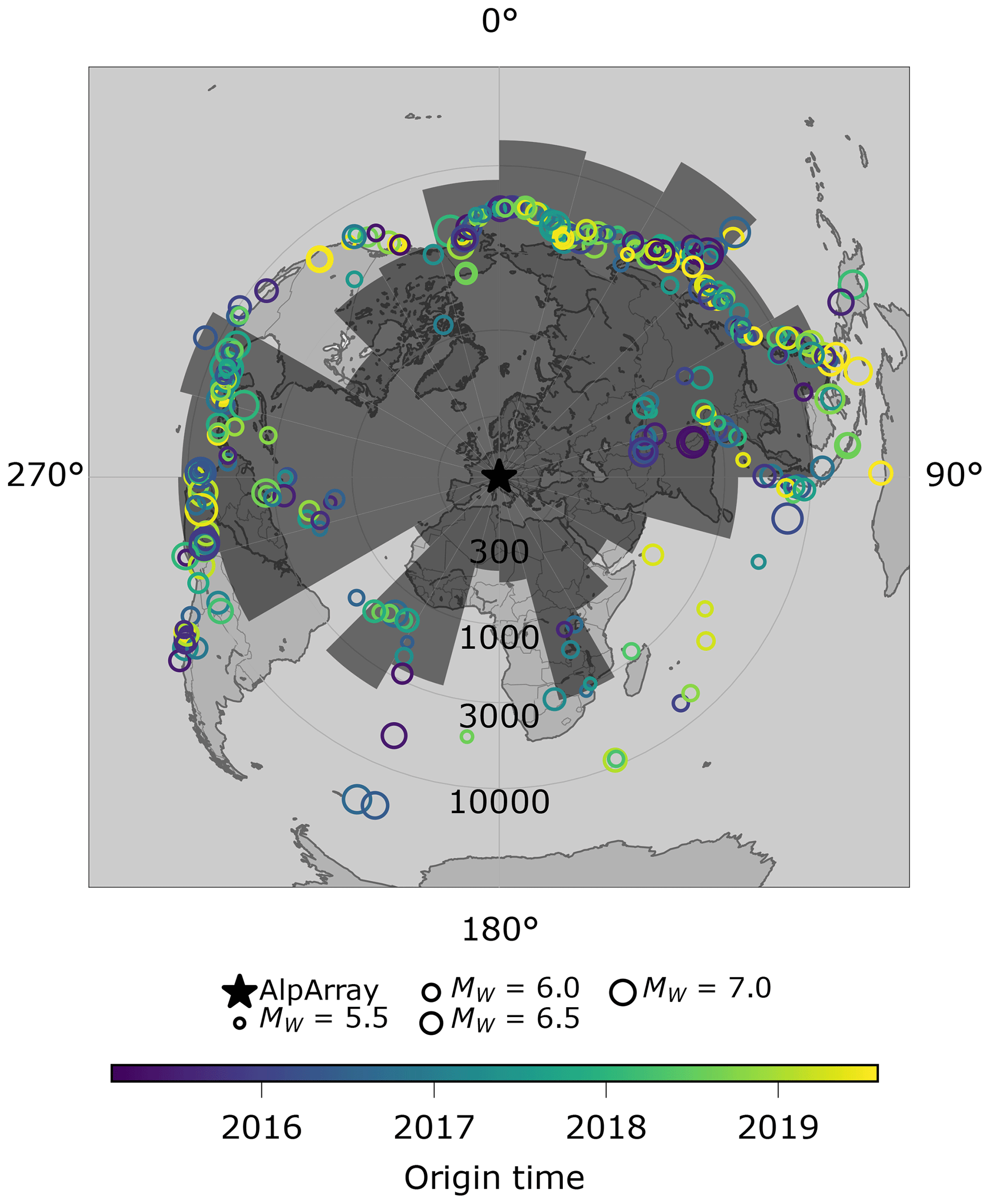
Figure 5Distribution of the picks of 331 events of the high-frequency dataset db0.5. Size of circles correlates with moment magnitude, colour with origin time. Histogram shows number of picks on the logarithmic radial axis binned in 15° bins azimuthally. The distribution is very irregular with most events located in the northeastern quadrant and in a western sector. There are large gaps with few events especially from the south and southeast as well as from the northwest resulting in a reduced number of picks from these directions. Peak value is 20 857 picks for the back-azimuth interval between 30 and 45°. The influence of the irregular distribution will get visible when analysing resolution capabilities and smearing of the set-up and can be seen especially well in the checkerboard test (Sect. 4).
Azimuthal distribution of events is strongly inhomogeneous (Fig. 5), with the majority of events coming from northeastern and western directions. There is a lack of events especially from southern directions, as well as from the southeast and northwest. This bias in azimuthal direction has to be taken into account when analysing results, as it might lead to smearing of different features in the direction of the least events, i.e. from northwest to southeast, an effect we will evaluate in detail later in a checkerboard test (Sect. 4).
Distances of events range from 35 to 135° to the centre of the array. Their distribution is also heterogeneous, scattering within only ±10 around 90° distance for back-azimuths between 270 and 40° and for the full range of up to ±50° for the remaining back-azimuths. However, we expect the influence of heterogeneity in distance distribution to be minor, as the maximum resulting difference in wave front incident angles does not exceed 13° at the surface and 29° at 600 km depth for a 1D earth model. Magnitude and origin time of the events do not show an azimuth or distance dependency except for a deficit of larger magnitude events in the southeast.
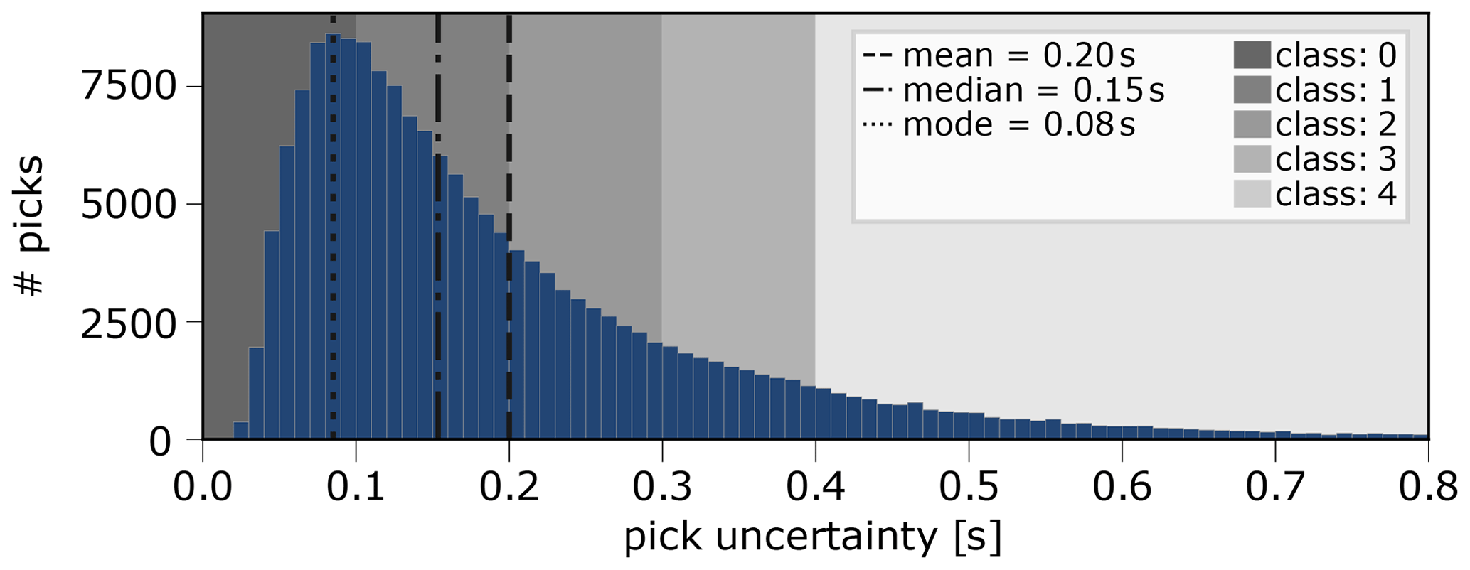
Figure 6Histogram of uncertainties of the full dataset as shown in detail in Paffrath et al. (2021a). Mean and median of uncertainties are indicated by vertical lines, as well as the bin with the highest number of pick uncertainties.
Travel-time uncertainties are categorized into five different classes in steps of 0.1 s ranging from class 0 (best) below 0.1 s to class 4 (worst), over 0.4 s. Although there is only a lower bound of the uncertainty for class 4, each onset in this class still has a well-defined uncertainty and will be used for the tomography. The travel-time uncertainty distribution of the dataset (Fig. 6) has a maximum at 0.08 s. The median of the distribution is 0.15 s, the mean is 0.2 s. Our average value of the estimated uncertainties is therefore lower than the one estimated by Lippitsch et al. (2003), who report a value of 0.36 s for 4199 P-wave travel times and larger than the one reported by Zhao et al. (2016), who estimate a value of less than 0.1 s for their 41 838 travel-time residuals. However, due to the high number of stations in the AlpArray project, our dataset contains over 46 000 (27 %) of the onsets in the highest class with an estimated uncertainty <0.1 s. Less than 10 % are in the lowest class of 0.4 s or higher. A detailed analysis of pick uncertainties also regarding the regional distribution can be found in Paffrath et al. (2021a).
The computation of a formal resolution matrix was not possible due to the size of the inverse problem. Instead, we perform resolution tests based on two sets of test models exhibiting anomalies of alternating sign arranged in 3D checkerboard patterns of different size separated by cubes with zero anomaly to analyse smearing effects. For constructing both test models, we start from the one-dimensional reference model shown in Fig. 4 (dotted line). At depths less than 100 km, we superimpose the velocity perturbations representing the lateral variations of our a priori crustal model but no checkerboard anomalies. At depths greater than 100 km we superimpose the checkerboard-like velocity anomalies only. In this way, we fully account for our a priori crustal model when calculating synthetic travel times for the resolution tests. Moreover, we add Gaussian noise to the synthetic travel times with a standard deviation given by the estimated uncertainties of the observed travel times. The inversion of the synthetic test data is performed in exactly the same way as the inversion of the observed data.
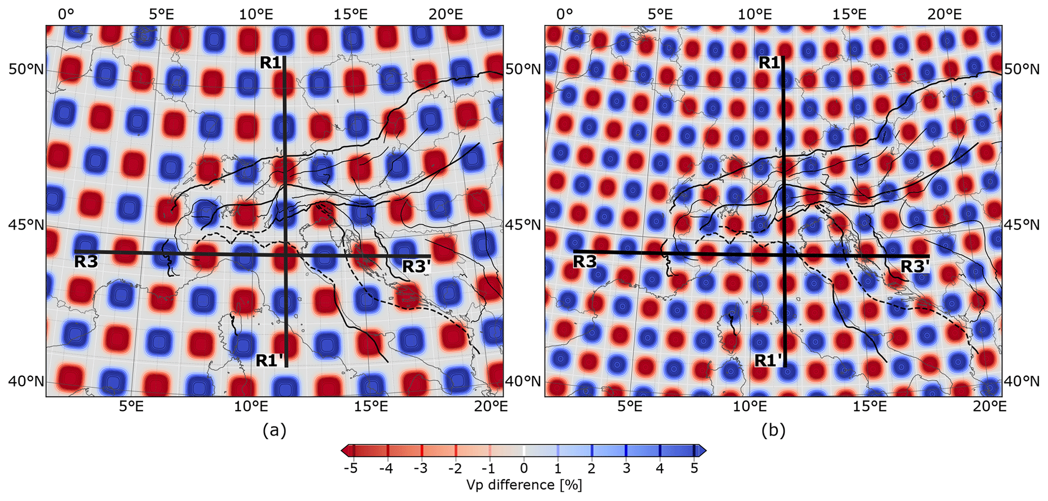
Figure 7Horizontal slice cutting through the centre of the uppermost anomaly layer of the two checkerboard models. Depth of the first slice (a) of the model is 150 km. Depth of the slice through the model (b) is 175 km.
The first checkerboard test model is made out of tiles covering grid points resulting in an average anomaly size of ca. km. The second checkerboard pattern is made out of tiles covering grid points creating anomalies of ca. km in size (Fig. 7b). Velocity perturbation is applied directly onto the inversion grid nodes, acting as a boxcar function. However, the spline interpolation in FMTOMO smoothes the edges of the anomalies, reducing the area of completely undisturbed space in between. For both patterns, the velocity perturbation reaches ±10 % at the tile centre (Fig. 7).
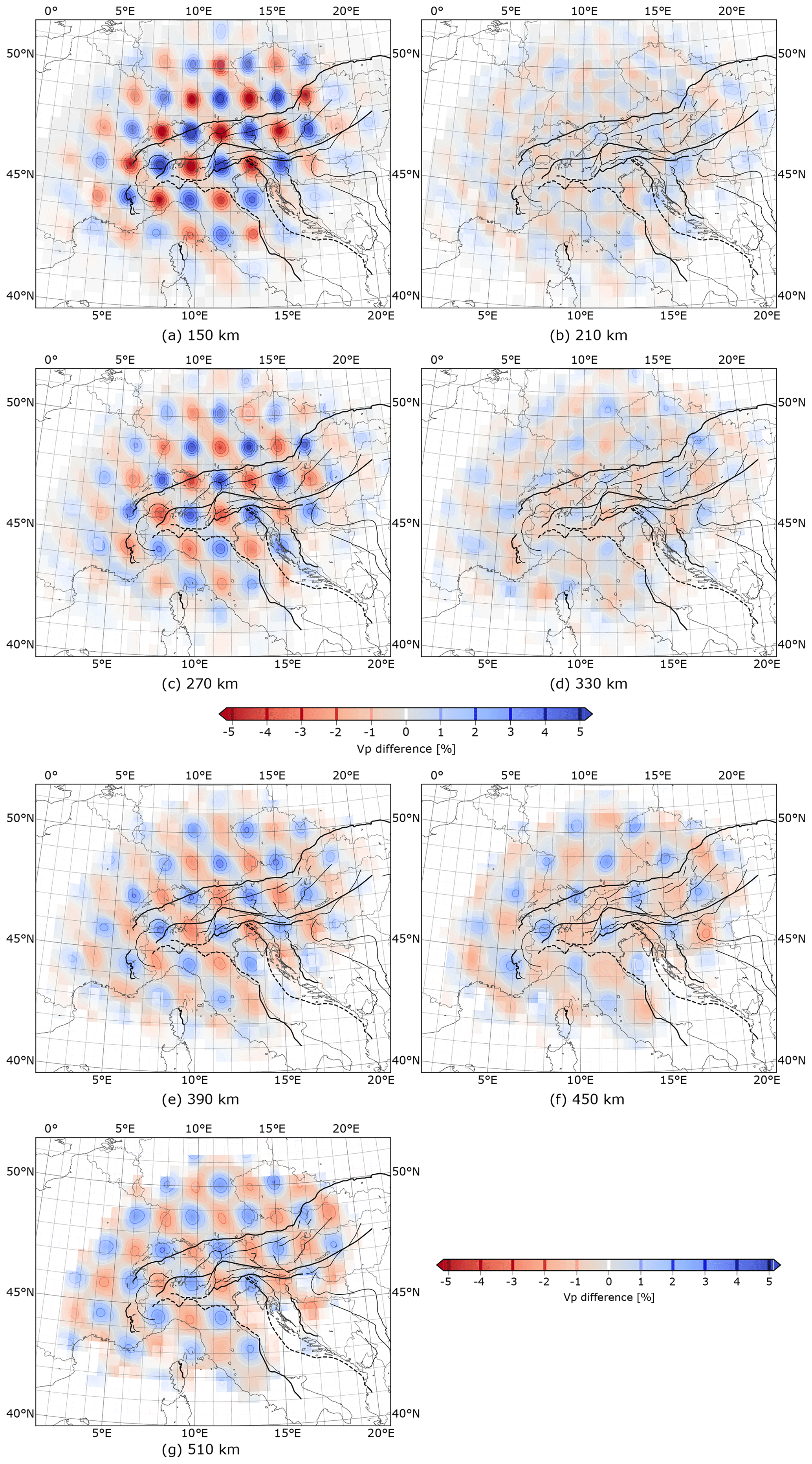
Figure 8Results of checkerboard analysis after 12 iterations for the grid. Misfit reduction is 87 %. Horizontal slices in the left panel cut through the maxima of velocity anomalies. Slices in the right column cut through the unperturbed spaces in between.
Figure 8 shows horizontal slices of the recovered checkerboard pattern at different depths. The slices in the left column always cut through the centre of the anomalies and the slices in the right column cut through the unperturbed spaces in between the tiles. For the shallowest depth of 150 km (Fig. 8a), test model recovery within well resolved areas is excellent. However, there is a slight decrease in amplitude with distance from the centre of the array. Some smearing effects are visible that connect areas with the same sign of velocity perturbation, preferably along a NW–SE direction. We explain this behaviour by the uneven event distribution (Sect. 3) that exhibits a strong deficit of earthquakes from SE and NW back-azimuths leading to much less ray crossings along the NW–SE direction compared to the NE–SW direction. For this reason lateral resolution along the NW–SE direction is reduced compared to the NE–SW direction.
At a depth of 210 km (Fig. 8b), the test model perturbation vanishes. Nevertheless, a weak velocity perturbation appears after inversion indicating slight vertical smearing. Amplitudes in the gap are by almost 1 order of magnitude smaller than at 150 km depth. At 270 km depth (Fig. 8c) the original checkerboard pattern is again clearly recovered, though we note a further decrease in the recovered amplitude. At 330 km depth (Fig. 8d) where the test model perturbation again vanishes, the recovered velocity perturbation is slightly stronger than at 210 km indicating a slight increase in smearing with depth. At 390 km depth (Fig. 8e), checkerboard recovery is still satisfactory but the recovered amplitude decreases further and NW–SE smearing becomes more prominent. The inverted velocity perturbation in the following zero perturbation layer of the test model at 450 km depth (Fig. 8f) assumes amplitudes comparable to the full anomaly layer above pointing to a further increased smearing. Remarkably, at the greatest depth of 510 km (Fig. 8g) the recovery of the anomaly pattern is still excellent, even though the size of well recovered anomalies grows well beyond 75 km owing to lateral smearing.
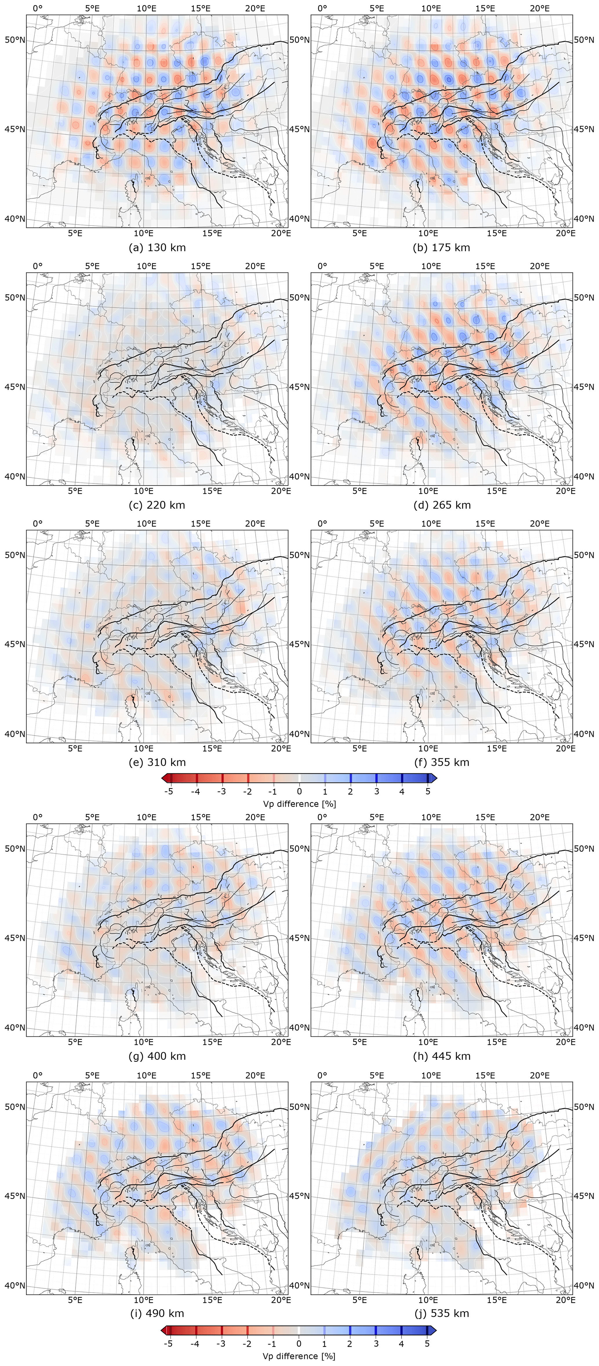
Figure 9Results of checkerboard analysis after 12 iterations for the grid. Misfit reduction is 72 %. Here, slices in the right panels cut through centre of velocity anomalies. Left panel slices cut through unperturbed space in between.
The reconstruction results for the checkerboard resolution test (Fig. 9) are less favourable. In contrast to Fig. 8, the horizontal slices through the gaps of the checkerboard pattern where the test model perturbations vanish are shown in the left column while the slices through the extrema of the test model perturbations are shown in the right column. At 130 km depth (Fig. 9a) where the test model is unperturbed, the inversion produces a velocity perturbation very similar to the one at 175 km depth indicating severe vertical smearing. This behaviour is due to the sub-vertical ray paths at shallow levels in the upper mantle that intersect at an acute angle leading to loss of vertical resolution. We estimate that the checkerboard anomalies are smeared vertically by at least 20 km at shallow depths below the crust (i.e. up to ∼150 km depth). This smearing effect highlights the importance of an accurate model of the crust and also the uppermost parts of the mantle from independent data.
At greater depths, e.g. in the following layer slicing directly through the perturbed test model at a depth of 175 km (Fig. 9b), the checkerboard pattern is well recovered. However, amplitude recovery is worse compared to the coarser checkerboard test model, and also vulnerability to NW–SE smearing is greater. In contrast to the uppermost unperturbed layer, the next one below at 220 km depth (Fig. 9c) is recovered much better due to the less steep rays at these depths. Smearing artefacts are faint, getting stronger close to the boundaries of the well irradiated model domain. The following perturbed layer at 265 km depth (Fig. 9d) is again recovered well but smearing of anomalies in the NW–SE direction connecting velocity perturbations of the same sign is more prominent. Below this depth, pattern recovery worsens systematically with depth. At 310 km (Fig. 9e), the unperturbed layer of the test model can still be distinguished from the perturbed ones but exhibits a clear imprint of the surrounding perturbed layers caused by smearing. Finally, for depths greater than 400 km (Fig. 9g–j) we can no longer distinguish between perturbed and unperturbed layers of the test model. Hence, we loose depth resolution for objects smaller than ∼50 km in size at those depths.

Figure 10Vertical slices of profile R1 (Fig. 7) cutting through the checkerboard models at 11.5° E. Shown are perturbations of P-wave velocity relative to the 1D reference model (Fig. 4, dotted line). (a, b) Test model used to calculate synthetic data including the a priori crustal model (crosshatched area). (c, d) Recovered checkerboard model including the slightly altered a priori model. Here we can analyse possible interactions between the resolved checkerboard perturbations and the overlying a priori model (e.g. connection of anomalies due to smearing). (e, f) Recovered checkerboard model with the a priori crustal model subtracted. Here we can analyse alterations of the crustal model (artefacts) due to mapping of the checkerboard anomalies into the crust.
Vertical slices through the checkerboard models (Fig. 10) on a N–S profile at 11.5° E further illustrate vertical and lateral smearing as discussed above. Additional vertical slices on a W–E profile at 44.5° N passing through the Ivrea body and the Po Plain can be found in the Supplement (Fig. S1). To check the vertical resolution in the crustal domain, we include a further checkerboard test where we did not add the perturbations of the crustal model but additional checkerboard tiles above 100 km (Figs. S2, S3).
The vertical cross sections in the top panels (Fig. 10a, b) show the perturbations relative to the one-dimensional reference model (Fig. 4, dotted line) that are used to compute the synthetic test data. As described above, they comprise the checkerboard-like perturbations applied at depths greater than 100 km and the perturbations representing the lateral variations of our 3D a priori crustal model applied at depths less than 100 km. There is a slight vertical elongation of the reconstructed anomalies of the checkerboard (Fig. 10c, d) in the uppermost level at ≈100 km depth indicating a reduction of resolution below crustal depths owing to sub-vertical ray paths. For both the coarse and the fine checkerboards, the original separation of positive and negative anomalies is better reconstructed at middle depth levels (200 to 400 km). There is also some diagonal smearing which is weak in the central regions but strong at the model boundaries reflecting the fact that teleseismic rays propagate obliquely through the model domain. If there is insufficient ray crossing, structures tend to become elongated parallel to the ray direction. This effect is best visible at the lateral model boundaries where crossing rays entering from the opposite side are missing but may also appear elsewhere if illumination from either side is strongly unbalanced.
To illustrate a potential leakage of the checkerboard anomalies into the shallow domain above 100 km depth, we subtracted the perturbations of our a priori crustal model from the reconstructed ones (Fig. 10e, f). As expected, the remaining anomalies are very weak indicating that the regularization of the inversion towards the a priori crustal model is very effective.
5.1 Setting global damping and smoothing weights
Starting from the a priori model of the crust and the uppermost mantle and the laterally homogeneous model of Fig. 4 (denoted by m0 in Eq. 5), we invert the dataset of travel-time residuals for P-wave velocity in the entire model domain. A priori standard deviations of P-wave velocity on the grid points are chosen as described in Sect. 2.4 for the crust and uppermost mantle. Below we choose a value of 15 % of the absolute velocity of the 1D background model. As resolution diminishes with depth, smoothing is increased with depth by weighting the rows of the matrix D in Eq. (5) with a linearly increasing factor between 1 (top) and (bottom of the model). For setting the global damping and smoothing weights as introduced in Eq. (5), we carried out a series of inversions with varying values of these quantities. The result are so-called trade-off curves that reflect the competing behaviour of misfit and model norm. We considered values for the damping weight of 3, 10, 30 and 100. Values of the global smoothing weight comprise 10, 18, 30, 56 and 100. For each combination of these two parameters, we obtain a value of the misfit and the model norm after 12 iterations. The resulting curves (Fig. 11) confirm the expectation that strong regularization leads to high misfit and low norm and vice versa. The ideal values of the regularization weights are those that provide the best compromise between the conflicting aims of low misfit and low model norm. Based on the results in Fig. 11, we choose the values of 10 for the damping and 30 for the smoothing weight.
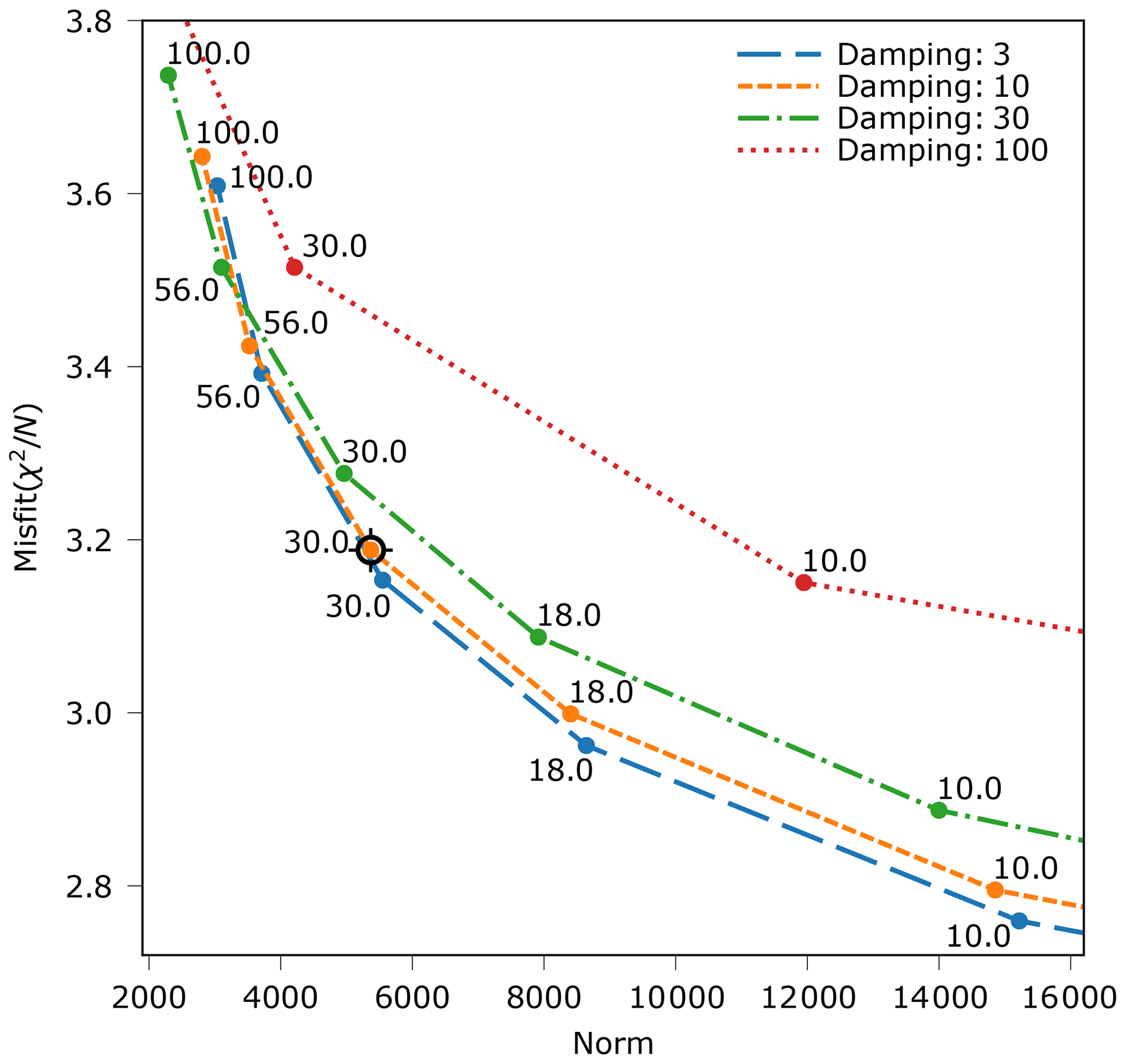
Figure 11Data misfit against model norm for different smoothing and damping parameters. Different damping parameters indicated by line and point colours. Smoothing parameters are written as text besides data points in the plot.
In principle, we want to reduce the average misfit to 1 in order to explain the data within their uncertainties. This criterion could be used to regulate the number of iterations to be done. However, our estimates of uncertainty might be too conservative or too optimistic. Moreover, the misfit is not only controlled by the data uncertainties but also by other factors. First, our solution of the forward problem has errors; second, ray theory is only an approximation to the full wave propagation problem; and, third, our model discretization does not admit all possible variations of P-wave velocity that may exist in the earth (including the ones outside the model domain). Hence, we expect additional deviations of the predictions from our measurements than the ones caused by the data uncertainty. As a consequence, a new criterion of when to terminate the iterative inversion is needed. Motivated by the basic aim of low misfit and low norm, we monitored both quantities with the iterations (Fig. 12) and find that the misfit drops quickly after the first few iterations and then decreases very slowly. The total norm also rises quickly and then levels off but continues increasing steadily with iterations. For the models shown in this section, we choose an upper limit of 12 iterations because beyond that we pay for additional marginal misfit reduction by an over-proportional increase in model norm. In addition, the smoothing norm saturates after 12 iterations. This fact indicates that further iterations increase the amplitude but only slightly alter the shape of the velocity perturbations.
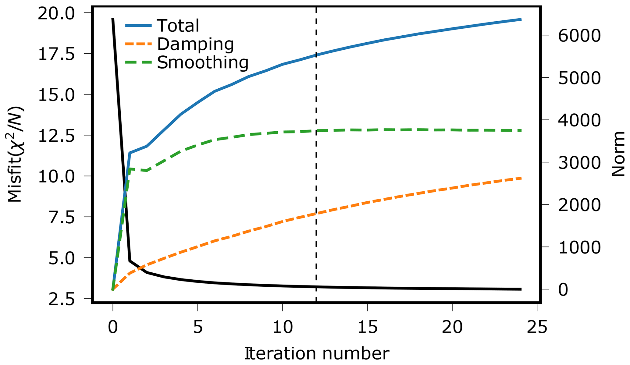
Figure 12Misfit reduction for 24 inversion iterations. Smoothing norm and damping norm are displayed by the green and orange lines; total norm is displayed in blue. We use the model after iteration 12 as our final model, as the misfit reduction becomes insignificant hereafter, whilst the smoothing term (model roughness) has reached its maximum and only the damping norm (model variation) continues to grow.
5.2 Visualization of the velocity model
In the following, we show horizontal and vertical cross sections through the final velocity model (Paffrath and Friederich, 2021). The figures show velocity perturbations relative to the 1D reference earth model (Fig. 4) including the velocity perturbations in the crust and uppermost mantle which are mainly controlled by our a priori crustal model.
In all cross sections, we overlay the velocity perturbations by a white shading that reduces intensity of the displayed colours. The amount of shading is chosen based on the illumination cells of the size of grid points by intersecting rays. To measure intersection, we define four azimuthal quadrants and count the number of rays hitting the cell from each quadrant. If there are 5 rays from each quadrant, the illumination quality of the cell is set to 1 and no shading is applied. For each quadrant with less than five rays, the quality factor is reduced by 0.25 down to 0 if all quadrants have less than 5 rays and shading is strengthened accordingly. In this way, the information about illumination and ray crossing in each cell of the inversion grid is conveyed to the model cross sections.

Figure 13Horizontal slices through the resulting model. Traces of vertical profiles are indicated at 180 km depth (and as thin grey lines on all profiles) where the major velocity anomalies can be seen best. Important anomalies discussed in the text are marked at 90 and 180 km depth.
5.3 Horizontal cross sections
The horizontal cross sections (Fig. 13) show velocity perturbations starting at a depth of 90 km and proceeding in 30 and 50 km steps down to 500 km depth. The most conspicuous structures in the model are the high-velocity anomalies appearing in the depth range from 150 to 210 km. They follow the Alpine chain and separate into three segments: a western one (C1), a central one (C2) and an eastern one (E). In addition, there is a fourth anomaly below the Apennines (A) that can be traced to the southeast into central Italy. Moreover, we define two other anomalies best visible at 90 km depth, (W) close to the Penninic Front and (D) in the northern Dinarides.
At 180 km depth, the fast anomaly (A) extends from the southern-central Po Plain in the north (10° E, 45° N) along the chain of the Apennines to central Italy (14° E, 42° N). At its northern end it is connected to anomaly (C1). Towards shallower depths from 150 to 90 km, it successively migrates to the west and loses amplitude in particular in its southern parts. At these depths, there is no connection to anomaly (C1) anymore. Below 180 km anomaly (A) keeps its lateral position down to 240 km depth but then moves successively to the west from 270 to 400 km depth. It splits and fades out below 400 km.
The anomaly (C1) which appears at 180 km depth beneath the westernmost part of the Po Plain migrates roughly in a NW direction towards shallower depths indicating a SE dip in this shallow part. At 90 km depth it is still recognizable but its velocity perturbation is about half of the one at 180 km depth. Below 180 km this anomaly migrates slightly to the south-southeast until about 300 km depth and develops a link to anomaly (C2) towards the northeast. Its amplitude decreases continuously with depth to finally vanish below 350 km.
Anomaly (C2) has its centre at 10.5° E and 46.5° N at 180 km. It becomes rather weak at 150 km depth and is replaced by a strong low-velocity anomaly at 120 km. At 90 km the velocity perturbation at the same position is still negative but weaker than at 120 km. The positive anomaly at 47.5° N and 9.5° E slightly to the NW of this location may be structurally associated with anomaly (C2). Between 180 and 350 km, anomaly (C2) slightly migrates towards the south-southwest, joins with anomaly (C1) to the southwest and becomes indiscernible at 400 km.
Anomaly (E) is centred at 47° N and 13° E at 180 km and stretches over 3° in longitude. It rapidly weakens at 150 km and is replaced by low velocities at 120 km depth. There is a small patch of elevated velocities to the west of the original location at 120 and 90 km depth which may be structurally related to anomaly (E). From 180 to 240 km depth, the anomaly keeps its intensity and exhibits a very marginal shift of its centre towards the east. At 270 and 300 km depth, it seems to split into a northern and a southern part that merge again at 350 km. The anomaly becomes indiscernible below 400 km.
In contrast to the strong high-velocity anomaly (A) beneath the Apennines, there is no comparable region of high velocities at the eastern rim of Adria beneath the Dinarides. Velocities there are normal to slightly positive except at 120 and 90 km depth where we obtain elevated velocities beneath the northernmost Dinarides (D) and also further to the SE.
Negative velocity perturbations generally surround the described high-velocity anomalies to the north, west and east in the depth range from 120 to 270 km. Low velocities also prevail in the same depth range to the south and southeast of the high-velocity anomalies stretching from the Po Plain into Adria. Exemptions from this general pattern are the strong low-velocity anomaly at 120 km depth located at 10.5° E and 46.5° N that separates the fast anomaly (C2) from shallower levels, and the extension of the low-velocity anomaly beneath the southeastern Po Plain to the NW, also at 120 km depth, that separates anomalies (A) and (C1). The low-velocity regions to the northwest of the fast anomalies (C1), (C2) and (E) tend to migrate to the southeast with depth. They are strongest at 90 and 120 km depth where they are located beneath the Black Forest in SW Germany and the Swiss Jura.
The described regular pattern of fast and slow anomalies dissolves at 350 km depth. Below, we obtain patchy but generally positive velocity perturbations beneath the entire Alpine region stretching from southern France to the Pannonian Basin. Low velocities are mostly restricted to the northern foreland and central Italy.
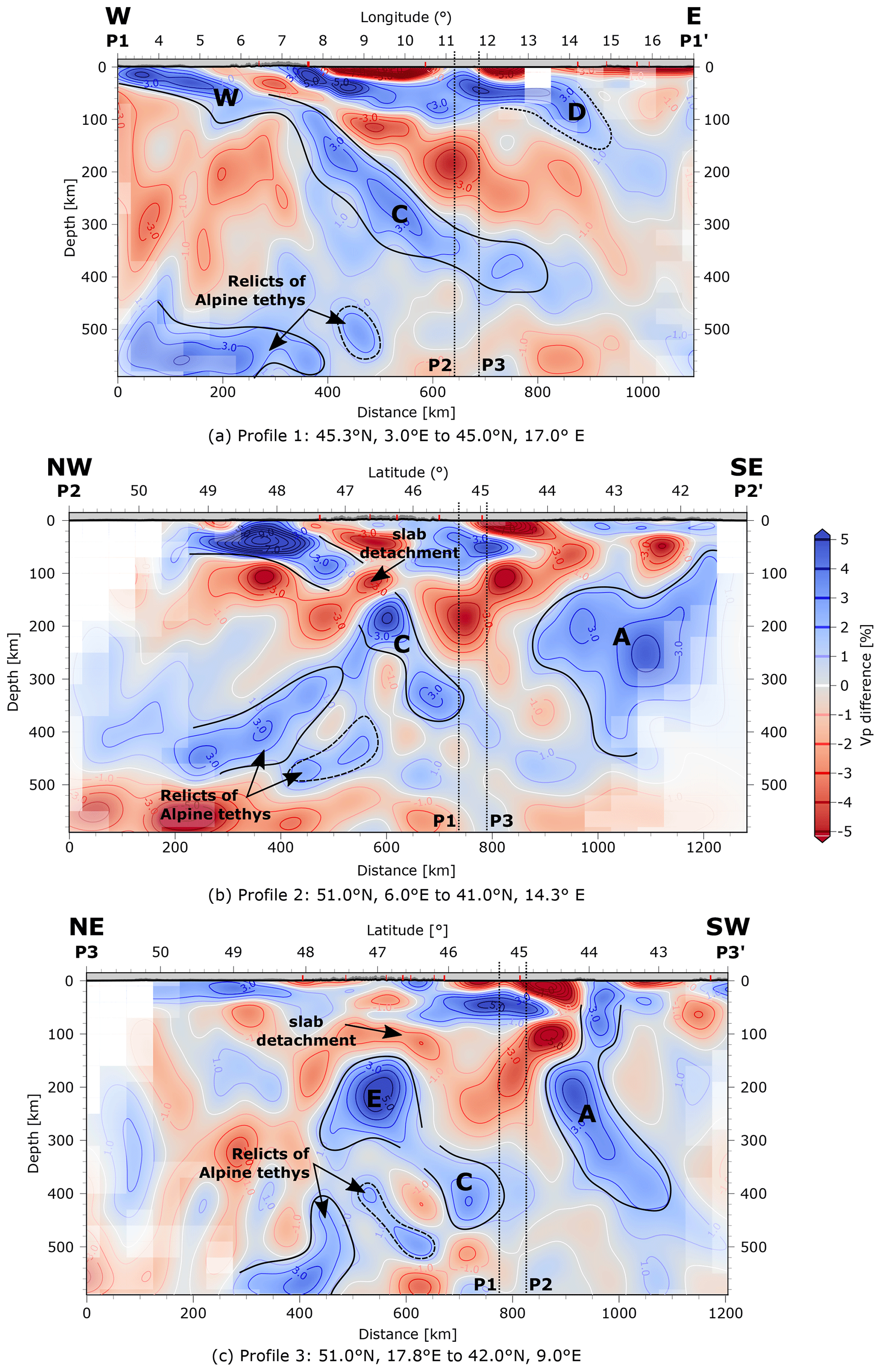
Figure 14Three vertical profiles cutting through the four major anomalies in the Alps and Apennines as indicated in Fig. 13d: (a) the western Alpine slab, (b) the central Alpine slab and (c) the eastern Alpine slab in the east, as well as the Apenninic slab in the west. Intersections between the different profiles are marked by vertical dashed lines. Distance in kilometres measured at the surface.
5.4 Vertical cross sections
We display three vertical sections (Fig. 14) through the resulting model that cut centrally through the major positive velocity anomalies in the Alps and Apennines at 180 km depth (Fig. 14). Moreover, profile P2 passes through the conspicuous low-velocity anomalies in the NW Alpine foreland at depths above 180 km and, of course, through the one directly located on top of fast anomaly (C2). All three profiles cross the strong low-velocity anomaly underneath the Po Plain appearing from 90 to about 270 km depth. The traces of the profiles are shown in Fig. 13d and as weak grey lines in all other figure panels.
Profile P1 (Fig. 14a) begins in SE France; crosses the western Alpine mountain chain, the Po Plain and the Adriatic Sea; and ends in the northern Dinarides. Its major feature is a high-velocity anomaly reaching from crustal depths in the westernmost part to depths of about 100 km close to the Penninic Front below the western margin of the Alpine mountain chain. Then, the anomaly becomes horizontal, weakens slightly and starts to dip again more steeply beneath the Ivrea body continuing in upward curved banana shape towards the east. Above this feature at crustal to uppermost mantle levels, separated by a strong low-velocity region, there are strong high-velocity anomalies, one associated with the Ivrea body and the other one with Adriatic lithosphere and possibly the northern Dinarides. Below the banana-shaped fast anomaly, at 8 to 9° E, there is a rather weak, steeply dipping high-velocity anomaly which may reach down to 500 km depth. At the bottom west of the section, there is a large, seemingly horizontal high-velocity anomaly.
Profile P2 (Fig. 14b) is NW to SE oriented and begins in the northwest at the western border of Germany, crossing the central Alpine mountain chain and the Po Plain until it reaches the Apennines and ends in southern Italy. It is directed along the main smearing direction as discussed in Sect. 4. Therefore, it is important to be aware of possible stretching of anomalies parallel to this profile. The main feature is the strong fast anomaly starting at crustal levels in the NW and dipping to the SE down to about 120 km depth. Directly below, dipping parallelly and with identical lateral extent, there is a rather strong low-velocity zone. The fast anomaly is interrupted by an about 40 km thick low-velocity region and then continues with a slightly stronger dip to about 360 km depth. To the SE above this anomaly, there is an extended low-velocity zone beneath the Po Plain that was already mentioned in context with profile P1. Above it, there is again a shallow high-velocity area associated with Adriatic lithosphere. Even further to the SE the profile touches the extended high-velocity anomaly beneath the Apennines.
Profile 3 (Fig. 14c) begins in southern Poland in the northeast, crosses the eastern Alps and the eastern Alpine high-velocity anomaly as well as the Apennines almost perpendicular to their strike, and ends in Corsica. It demonstrates that the strong positive anomaly (E) appearing below 150 km is connected neither to European lithosphere in the NE (between 50 and 48° N) nor to Adriatic lithosphere in the SW between 46 and 44.5° N. Its southwestern extension more likely belongs to anomaly (C) defined in profile P2. There is a potential vertical continuation of anomaly (E) that splits into a part dipping SW and another stronger part dipping NE. Further to the SW, the profile intersects the high-velocity anomaly beneath the Apennines (A) that is well separated by a region of very low velocities from shallow Adriatic lithosphere further to the NE. Anomaly (A) is connected to the crust, dips nearly vertically with a slight tendency towards the NE in the shallow mantle and then overturns towards SW below 200 km.
6.1 Interpretation of velocity perturbations
6.1.1 High-velocity anomalies
We follow the petrophysical and geodynamical arguments of previous authors (Lippitsch et al., 2003; Mitterbauer et al., 2011; Piromallo and Morelli, 2003; Spakman et al., 1993) and interpret the high-velocity anomalies as associated with lithospheric material subducted during the different stages of the collision of Europe and Adria. The fast anomalies defined in the horizontal and vertical sections above correspond to the Adriatic slab beneath the Apennines (A), a central, arcuate slab following the western end of the Periadriatic Fault System (PFS) of presumably European origin (C1, C2), and a slab in the eastern Alps (E) whose provenance is currently debated due to conflicting images of its dip (Lippitsch et al., 2003; Mitterbauer et al., 2011) and the Moho geometry (e.g. Waldhauser et al., 2002; Spada et al., 2013) leading to hypotheses of a possible slab polarity switch in this area (Lippitsch et al., 2003; Schmid et al., 2004; Kissling et al., 2006; Luth et al., 2013; Handy et al., 2014). These anomalies are clearly visible as rather well-separated entities in our model in the depth range from 150 to 240 km but lose their individual identity at both smaller and greater depths. Hence, attributing these anomalies to lithospheric slabs of European or Adriatic provenance is subject to interpretation (e.g. Handy et al., 2021, this volume) and should also be based on additional evidence. The shallow fast anomaly (W) close to the Penninic Front is interpreted as the western Alpine slab. Anomaly (D) indicates shallow subducted material beneath the northern Dinarides. The widespread high-velocity anomalies at the bottom of the model underlying the entire Alpine chain are presumably relics of the Alpine Tethyan ocean.
6.1.2 Low-velocity anomalies
Low-velocity anomalies are generally attributed to warm asthenospheric mantle. However, as discussed in detail in a companion paper by Handy et al. (2021), the distribution of low velocities in our model (horizontal sections at 120 to 210 km depth; Figs. 13b–e and 14b indicate a dichotomy in the character of low velocities in the western and eastern Alpine region. Handy et al. (2021) postulate that the low-velocity volumes extending into the western and northwestern foreland are part of a thick lithosphere that is inherited from pre-Alpine domains. It is attached to the base of the dipping slabs and appears to exhibit the same kinematic behaviour.
Alternatively, these low-velocity volumes could be related to seismic anisotropy (e.g. Bezada et al., 2016). Studies of seismic anisotropy in the Alps indicate a polarization of the fast SKS shear wave approximately parallel to the curvature of the Alpine belt (e.g. Barruol et al., 2011) with maximum anisotropy magnitude in the external units. This finding implies a horizontal preferred orientation of the fast axis of rock forming minerals along that direction somewhere in the mantle below these areas. As a consequence, steeply incident teleseismic P waves passing through these mantle regions tend to be slower than the isotropic average because they propagate nearly perpendicularly to the fast axis. Thus, the conspicuous belt of low velocities at depths around 150 km (Fig. 13b–d) below the foreland of the western part of the Alpine chain up to a longitude of about 10° E may be due to anisotropy caused by asthenospheric mantle flow around the Alpine slabs.
Bezada et al. (2016) analyse the effect of anisotropy on isotropic teleseismic P-wave tomography. Their results confirm our view. They consider three different azimuthal distributions of seismic events and find for a sub-horizontal fast symmetry axis that (Sect. 4 of their paper) azimuthal coverage is of secondary importance when dealing exclusively with teleseismic arrivals and that the primary factor is the sub-vertical orientation of the teleseismic ray paths and their consequential sampling of the slower directions of regions with sub-horizontal fast axes.
Anisotropy may also contribute to the observed low velocities east of 10° E but new XKS-splitting results of Link and Rümpker (2020) indicate that it becomes weaker east of the Tauern window. Therefore, low velocities below the eastern Alps and the Carpathians are preferentially interpreted as upwelling asthenospheric material associated with a large-scale delamination of European lithosphere and orogen-parallel eastward extrusion of the eastern Alpine and Carpathian crustal edifice. Also, the low-velocity region below the Po Plain presumably represents asthenospheric upwelling combined with a contribution due to hydration related to the position of this anomaly above the descending thick European lithosphere (Giacomuzzi et al., 2011).
6.1.3 Western Alpine slab
One issue regarding the interpretation of the fast anomalies concerns the depth extent and continuity of the slab beneath the western Alps. Based on the vertical section along profile P1 (Fig. 14a), we argue for a relatively short (130 km), shallow western Alpine slab derived from the European lithosphere ending at about 100 km depth close to the Penninic Front. A slab length of about 130 km fits well with the W–E component of the displacement path taken by the most internal part of the European crust in this area (the present-day Gran Paradiso massif) with respect to stable Europe (Schmid et al., 2017). The banana-shaped fast anomaly following further east more likely represents the central Alpine slab which is cut by profile P1 obliquely to its roughly southeastward dip direction. The steeply dipping areas of elevated velocities beneath the banana-shaped anomaly are weak and we refrain from interpreting them as a possible continuation of the western Alpine slab. With this interpretation, we deviate from Zhao et al. (2016), who interpret this deep-reaching fast anomaly as part of the western Alpine slab. It is more likely that the scattered areas of positive velocity anomalies at great depths represent relics of the Alpine Tethys. This interpretation is supported by the patchy but widespread fast anomalies covering the entire Alpine region at depths below 400 km. We also deviate from the interpretation by Kästle et al. (2020), who interpret the banana-shaped anomaly as a western Alpine slab and postulate a break-off at around 100 km depth.
6.1.4 Central Alpine slab
The interpretation of a short western Alpine slab implies that the fast anomaly (C1) appearing from 150 to 240 km depth structurally belongs to the central Alpine slab which comprises the fast, arc-shaped anomalies following the Periadritic fault system from about 8 to 10.5° E visible from 90 to 300 km depth (Fig. 13). Its easternmost part is featured in profile P2 (Fig. 14b). In this profile, the slab has a gap at about 120 km and continues below 160 km down to about 400 km with a steep southeastward dip. Below the shallow part of the slab, we find a low-velocity zone following the slab dip and interpreted by Handy et al. (2021) as the lower part of thick European lithosphere comprising layered high- and low-velocity anomalies. Detachments further to the west of the profile are not as clear as the slab anomaly is not intersected by low-velocity areas but only weakens laterally and seems to split into two vertical arms below 150 km depth in order to merge again below 240 km depth (Fig. 13b–f).
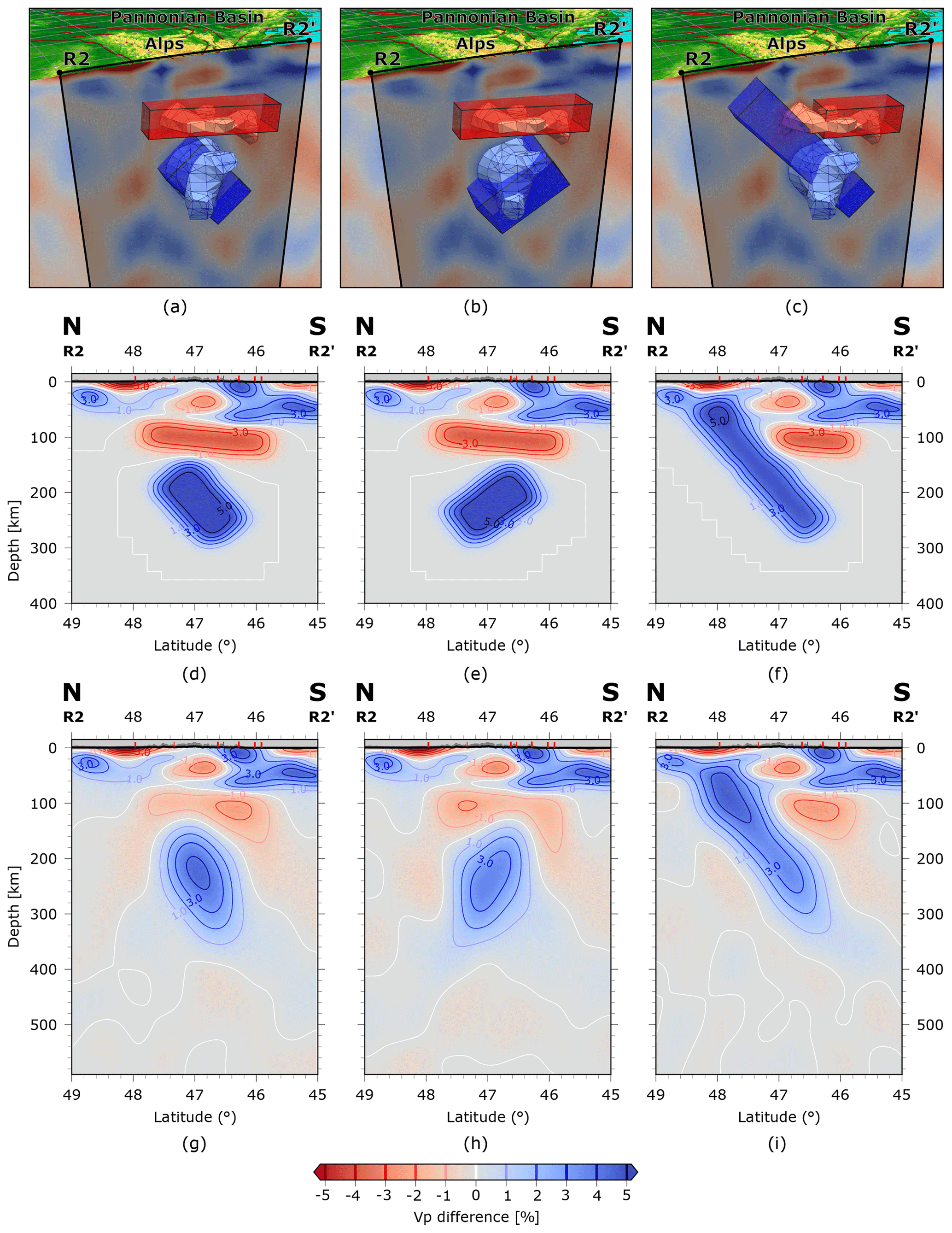
Figure 15Resolution analysis for profile E at longitude 13.3° E. (a, b, c) 3D models of the three different test cases for (a) a delaminated slab dipping to the south, overlain by a low-velocity zone; (b) an identical case but with a northward-dipping slab; and (c) a slab connected to the European lithosphere with a low-velocity zone representing upwelling mantle. Meshed volumes show velocity perturbation iso-surfaces of P-wave velocity increase of 2 % of the actual model results. Semi-transparent rectangular boxes show positions of the modelled anomalies for the resolution test. (d, e, f) Vertical profile through the resulting spatially smoothed synthetic slabs, after importing them into the velocity grid. (g, h, i) Recovered structures after 12 inversion iterations.
6.1.5 Eastern Alpine slab
In contrast to the central Alpine slab, the eastern Alpine slab associated with the easternmost fast anomaly (E) at 180 km depth (Fig. 13) is completely detached and replaced by warm mantle above 150 km depth. The slab featured in profile P3 is very prominent between 200 and 300 km depth but weakens at greater depths and seems to split into two branches, a stronger northern and a weaker southern one. This behaviour may produce the overall impression that anomaly (E) dips slightly towards NE. We have carried out a dedicated resolution test to check if the detachment of the slab can be resolved by our data (Fig. 15). For this purpose, we created test models containing an elongated, box-shaped low-velocity perturbation of 3% underlain by a fast, also box-shaped anomaly of up to 5%. In test models (a) and (c), the fast box dips towards S, in test model (b) towards north. The low-velocity box in test models (a) and (b) completely overlies the fast anomaly while in test model (c) the fast anomaly reaches up to the crust. Besides the test structures, the models also contain the velocity perturbations of our a priori crustal model. From the test models, we computed synthetic travel-time residuals, added Gaussian noise and inverted them using the same parameters as in the original inversion. In all cases we notice a general decrease in the anomaly amplitudes due to regularization of the inversion. In the case of the detached slabs (Fig. 15d, e) the shape of the anomalies can be reconstructed well. However, the recovered detached slabs exhibit a stronger dip than the test structures especially for the N-dipping slab. Reconstruction is best for the S-dipping attached slab. We conclude from this result that we can resolve the detachment but may miss a steep northward dip of the slab.
Regarding the provenance of the eastern Alpine slab one might be tempted to postulate a structural connection to the Adriatic lithosphere in the SW instead of one to the European lithosphere in the NE. This cannot be decided from this tomography alone. However, Handy et al. (2021) argue for a European provenance of the slab as its down-dip length (300–500 km) matches the estimated Tertiary shortening in the eastern Alps accommodated by originally south-dipping subduction of European lithosphere.
6.1.6 Adriatic slab
The largest high-velocity anomaly in our model is the Adriatic slab beneath the Apennines that is cut perpendicularly by profile P3 (Fig. 14c). There, the slab exhibits a nearly vertical to slightly NE-directed dip down to about 140 km and then dips towards SW. The latter dip direction is expected from plate tectonic reconstructions (Jolivet and Facenna, 2000) that describe a retreat of the Adriatic slab towards the east. The steepening of the slab at shallow depths may be related to the termination of the advancement of the Apennines in Plio-Pleistocene time (Handy et al., 2021). The Adriatic slab attains its greatest lateral extent below 180 km depth where it reaches well into central Italy (Fig. 13) reaching the southern limit of our model close to 41°N. Towards shallower depths, its SE-ward limit is systematically shifted towards NW. At 90 km depth its SE end is north of 43°N. This behaviour indicates a detachment of the slab south of 43°N. Full attachment of the slab to the crust seems to be restricted to its northernmost parts, being a potential reason for the overturning of the slab in its northern part because it inhibits or at least impedes a further eastward retreat of the slab. Remarkably, despite having exhibited a dip in opposite directions in the Miocene (Jolivet and Facenna, 2000), the Adriatic slab and the SW part of the central Alpine slab merge at depths greater than 180 km where they exhibit a nearly vertical dip. However, both are clearly separated partially by low-velocity regions at shallower depths.
6.1.7 Dinarides
With regard to the Dinarides, our model indicates a shallow slab only in their northernmost part as discussed in Handy et al. (2021). The high-velocity signature below 150 km along the Dinaridic chain is very weak and vanishes below 240 km. It should, however, be noted that resolution degrades in this part of model. In addition, the a priori crustal model is less reliable there than in the core region of the Alps.
6.2 Comparison with previous studies
The results of our study can be directly compared to the previous studies by Lippitsch et al. (2003), Koulakov et al. (2009), Mitterbauer et al. (2011) and Zhao et al. (2016), who investigated approximately the same region with data available before the installation of the AlpArray Seismic Network.

Figure 16Comparison of the results of this study with the models of Zhao et al. (2016) (left column) and Koulakov et al. (2009) (right column). Contour lines of our model are plotted for each 1 % change in P-wave velocity on top of the results of Zhao and Koulakov (shaded colours). Grey colours show areas where Zhao and Koulakov do not provide P-wave velocity values.
In particular the study by Zhao et al. (2016) encompasses the same region as covered in this study. The focus of the study by Mitterbauer et al. (2011) lies in the eastern Alpine region while Lippitsch et al. (2003) concentrate on the core region of the Alps. The study by Koulakov et al. (2009) considers all of Europe and exhibits less resolution and smaller velocity perturbations. Since the models by L. Zhao (personal communication, 2021) and Koulakov et al. (2009) are available digitally, we show a direct comparison with our model along the three profiles P1 to P3 in Fig. (16). For simplicity, we also refer to the models resulting from these studies as Lippitsch's, Koulakov's, Mitterbauer's and Zhao's in the following.
Remarkably, all studies agree nearly perfectly in their velocity anomalies in the depth range around 200 km showing the high-velocity anomalies (C1), (C2) and (E) at the same locations. In the models by Lippitsch et al. (2003) and Mitterbauer et al. (2011) (only anomalies (C2) and (E) because (C1) is outside the model domain), these anomalies appear well separated as in our study while they seem laterally connected in the model of Zhao et al. (2016).
Models start to differ from each other at depths below about 250 km. For example, the three strong anomalies (C1), (C2) and (E) start to weaken and disappear at 270 km in Lippitsch's model while they prevail down to at least 350 km in our model. This leads to a higher estimate of the length and penetration depth of the slabs. Similarly, Mitterbauer's model looses track of the (C2) anomaly below 250 km. Their eastern Alpine slab looks coherent to great depths while in our model it develops a complicated internal structure.
The vertical sections in Fig. 16 demonstrate that the good agreement of our model with Zhao's extends to about 400 km depth and also includes the location and shape of the Adriatic slab (anomaly A). Except for some details, the distribution of high and low velocities in this depth range is identical in all three profiles. One such detail is the positive anomaly in profile P2 beginning at anomaly (C) and descending to the NW interpreted by us as a relict of Alpine Tethys which is not present in Zhao's model. A second one is the banana-shaped anomaly (C) in our model which appears less continuous in Zhao's model. Koulakov's model exhibits less detail and less strong anomalies but still the distribution of high- and low-velocity anomalies agrees rather well from the surface down to at least 300 km. Similarities beyond 400 km depth with Zhao's and Koulakov's models are the high-velocity regions underneath the entire Alpine chain between 400 and 500 km depth as well as the deep-reaching European and Adriatic slabs.
All models diverge from each other in different ways towards shallower depths. In Lippitsch's model, both anomalies (C2) and (E) are continuous up to 90 km depth while anomaly (C1) disappears at 120 km and reappears at 90 km. In particular, the upward continuity of anomaly (E) and its connection with fast Adriatic lithosphere to the SW in Lippitsch's model lead to the interpretation of a NE-dipping slab of Adriatic provenance, also implying a polarity switch from the SE-dipping central Alpine slab to the NE-dipping eastern Alpine slab. In contrast, in Zhao's and Koulakov's models, only anomaly (C1) reaches the upper limit of the model while anomalies (C2) (Fig. 16c, d) and (E) (Fig. 16e, f) weaken significantly towards the surface. In Koulakov's model, there is a transition to low velocities above anomaly (C2) at around 80 km depth. Thus, the low-velocity anomaly at about 120 km depth in our model interrupting the central Alpine slab in its easternmost part is rather unique. Nevertheless, neither Zhao's nor Koulakov's model excludes a potential detachment there.
The eastern Alpine slab (anomaly E) appears to be nearly vertical in both Zhao's and Koulakov's models. This finding is corroborated by Mitterbauer's model where anomaly (E) also weakens with decreasing depth and appears to keep its lateral position indicating a rather vertical slab with weak or no connection to the crust and therefore not requiring a polarity switch. In our model, the fast anomaly (E) completely disappears at depths less than 120 km indicating a complete detachment. The dip is sub-vertical and, hence, does not require a polarity switch either. Given the big amount of subducted material, Handy et al. (2021) argue for a European provenance of the slab as southward crustal shortening in the southern Alps is only about 50 km. Thus, the more plausible interpretation is that there is only one European slab, most of which is detached from the orogenic crust.
The fact that the various models exhibit significant discrepancies particularly at shallow depths raises the question of the role played by crustal corrections. All models differ in the crustal models available for correction and how the crustal corrections are applied. The previous studies directly apply the corrections to the observed travel times either assuming vertical wave propagation through the crust or calculating travel-time corrections for each event separately. The role of crustal corrections in Koulakov's model is unclear as Koulakov et al. (2009) apply an inverse teleseismic scheme with sources in the study area and receivers worldwide. In contrast, we integrate the a priori crustal model into the initial model and allow modifications during the inversion. Moreover, our study is the only one that uses an a priori model of the crust and uppermost mantle based on a tomographic study using local earthquakes.
If applied directly to the travel times, a priori crustal corrections may create compensating structures in the mantle below especially if they are in conflict with the observed teleseismic travel times. For example, a wrong low-velocity anomaly in the crust would produce a compensating high-velocity anomaly in the mantle below and vice versa. In this case, it is beneficial that teleseismic inversion is allowed to change the structure of the crust as well.
A further effect that may add to discrepancies at shallow levels is the fact that in teleseismic tomographies vertical resolution tends to diminish towards shallow depths. It can be expected that tomographies based on sparser networks may be more sensitive to vertical or oblique smearing at shallow depths compared to others thereby worsening the tendency to image continuous vertical or dipping structures. Nevertheless, even with the data from the AlpArray Seismic Network we must rely on the a priori crustal model to be able to make robust statements about slab detachment and delamination.
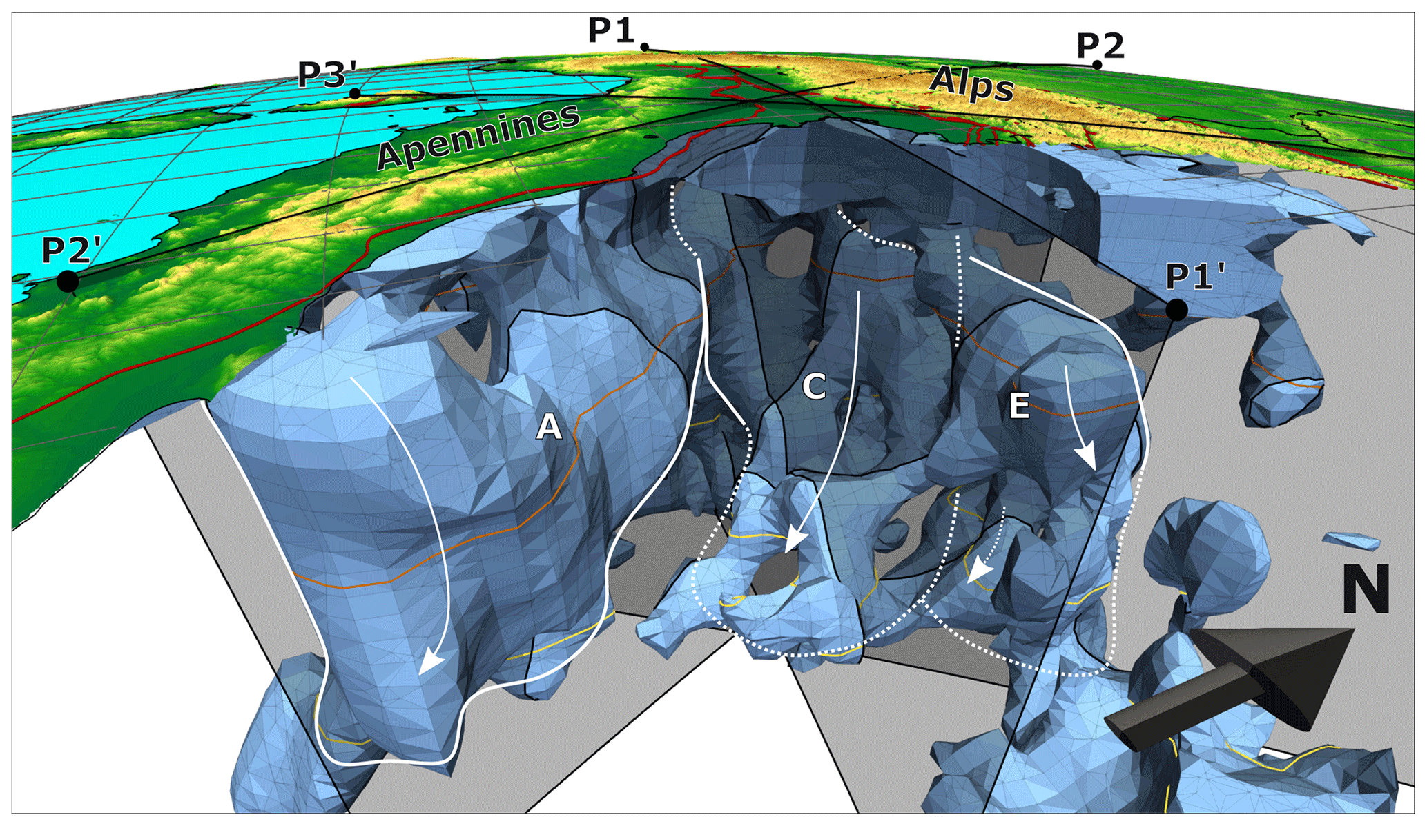
Figure 17Three-dimensional view from the southeast (Adria) into the resulting model after 12 inversion iterations. We show here velocity iso-surfaces for an increase of 1.25 % in P-wave velocity. High-velocity structures in the SE that would block the view have been clipped. The three vertical profiles P1, P2 and P3 are indicated as semi-transparent surfaces as well as the respective contours of the iso-surfaces along these profiles (black lines). The 410 km discontinuity is shown as a thin yellow line on the anomalies, as well as the outline of the horizontal slice at 180 km depth (thin brown line). Associations of the 3D high-velocity bodies with the interpreted slabs and the velocity anomalies (A), (C) and (E) defined in the horizontal and vertical cross sections are indicated by white lines.
6.3 A 3D view of the slab configuration beneath the Alps
Instead of providing a hand-drawn representation of the 3D configuration of the slabs in the greater Alpine region as in Handy et al. (2021), Zhao et al. (2016) or Kästle et al. (2020), we display here a 3D figure directly created from our model showing the outer boundaries of volumes in the model whose velocity perturbation is greater than or equal to 1.25 % (Fig. 17). The purpose of this figure is to provide a realistic impression of the complex and irregular shape of the slabs. Admittedly, the choice of a velocity threshold is subjective and the image would change if a different one was chosen. Nevertheless, slab sketches produced from tomographic results are also often based on a velocity threshold, and the definition of slab boundaries is entirely subjective as well. Moreover, for physical reasons, we cannot expect a sharp slab boundary, as the slab is in a process of thermal equilibration with its surroundings and any potential discontinuous initial temperature contrast will be smoothed by thermal diffusion.
We have chosen a view from the SE that allows the visualization of all the major slabs (except the western Alpine one) discussed in this paper. High-velocity structures in the SE that would block the view have been eliminated. Many of the features discussed above can be recognized in this figure, for example, the central European slab going down to 410 km depth (indicated by the thin yellow line) thereby decreasing its dip angle, bifurcating around 180 km depth (indicated by the thin brown line) and again merging at shallower depths; the detachment of parts of the central and the entire eastern Alpine slab; the partly overturned Adriatic slab detached in its southern parts but still attached further north and separated at shallow depths by a little hole from the European slab; and the merging of the central Alpine and Adriatic slab at greater depths. The western Alpine slab is not visible as it is hidden by the central one. The 3D view demonstrates that our common perception of slabs as thin, regular sheets with planar or neatly curved surfaces shown in schematic drawings in textbooks is too simplistic and idealized. Real slabs may have an irregular shape, exhibit corrugated and torn surfaces with holes and gaps and may show strong variations in thickness.
We note that figures like Fig. 17 image positive velocity anomalies, not necessarily entire slabs. Negative anomalies are omitted, even though some slabs may comprise both positive and negative anomalies, e.g. in the downward-moving European slab of the Central and western Alps. The reader is referred to Fig. 11 in Handy et al. (2021) for an integrative, if schematic view of the orogenic lithosphere and slabs in their entirety, as seen from the same vantage point as Fig. 17.
Based on the wealth of waveforms recorded by AlpArray, we have been able to extract an exceptionally large dataset of high-quality teleseismic travel times and travel-time residuals from which the new exciting images of mantle structure beneath the greater Alpine region and the Apennines presented in this study are derived.
AlpArray waveforms proved to be particularly well suited to enhance travel-time determination by array methods such as beamforming and cross-correlation that are required to fully exploit the resolution capabilities offered by such an array. Thanks to the long recording time, it was also possible to obtain recordings from azimuthal sectors with very low teleseismic activity.
We have made particular efforts to compile the most recent and reliable information on P-wave velocity structure of the crust and uppermost mantle in the study region, which is essential to make inferences on the nature of coupling of the slabs with the plates at the surface. In contrast to previous studies, the travel-time data were not directly corrected for crustal effects but instead the a priori crustal model was incorporated as initial model into the teleseismic inversion. By defining a priori standard deviations for the initial model, the inversion is regularized towards the a priori model but may deviate from it if demanded by the data. In this way, we can avoid or reduce undesired compensation effects if the a priori model proves to be incorrect.
The new detailed images of slab configuration beneath the greater Alpine region and the Apennines exhibit differences to previous studies in different places leading to a substantial change of the structural interpretation. The western Alpine slab is short and ends at about 100 km depth. Its apparent extension to the east and to greater depths interpreted by other authors is rather due to the central Alpine slab that extends to the south at greater depths. The central Alpine slab follows roughly the curved western end of the Periadriatic Fault System and bifurcates into two branches at depths between 150 and 250 km. Contrary to previous work, it is detached at its eastern end by a horizontal slab tear at about 120 km depth. There is a little gap between the central and eastern Alpine slab located beneath the western rim of the Tauern window. Also in contrast to previous work, the eastern Alpine slab is completely detached from the orogenic root and develops its full extent at around 180 km depth. The separation of central and eastern slab becomes unclear below 250 km depth. Both slabs dip very steeply and exhibit connections to subducted material at the bottom of the model presumably representing relics of the subducted Alpine Tethys. The new model does not require a subduction polarity switch due to the detachment from the crust and the nearly vertical dip of the eastern Alpine slab. Tectonic arguments rather suggest a European provenance of the slab. Thus, all high-velocity zones, as well as potentially some low-velocity zones in the European lithosphere (Handy et al., 2021, this volume) imaged along the Alpine mountain belt represent subducted material of European origin. Large amounts of subducted Adriatic lithosphere are found only beneath the Apenninic mountain range reaching great depths and showing a slight overturning from NE to SW dipping mainly in its northern part where it is still attached to the crust. Further to the SW, the Adriatic slab is detached by a horizontal tear that seems to deepen towards the SW.
The slow anomalies in the model exhibit an interesting spatial pattern that suggests a dichotomy of the properties of the upper mantle between the western and northern and between the eastern and southern regions of the study area. In the west and north, slow anomalies dip in parallel with fast anomalies hinting at a very thick downward-moving lithosphere of about 150–180 km thickness that may be inherited from Variscan or pre-Variscan structures. Alternatively, these low-velocity regions may signify the presence of anisotropy caused by asthenospheric mantle flow around the Alpine slabs. In contrast, in the east and south, Adriatic lithosphere is comparably thin and underlain by warm asthenosphere influenced in the south by a potential hydration of the mantle behind the European slab or, in the east, by eastward extrusion and thinning of the lithosphere owing to the retreat of the Carpathian slab.
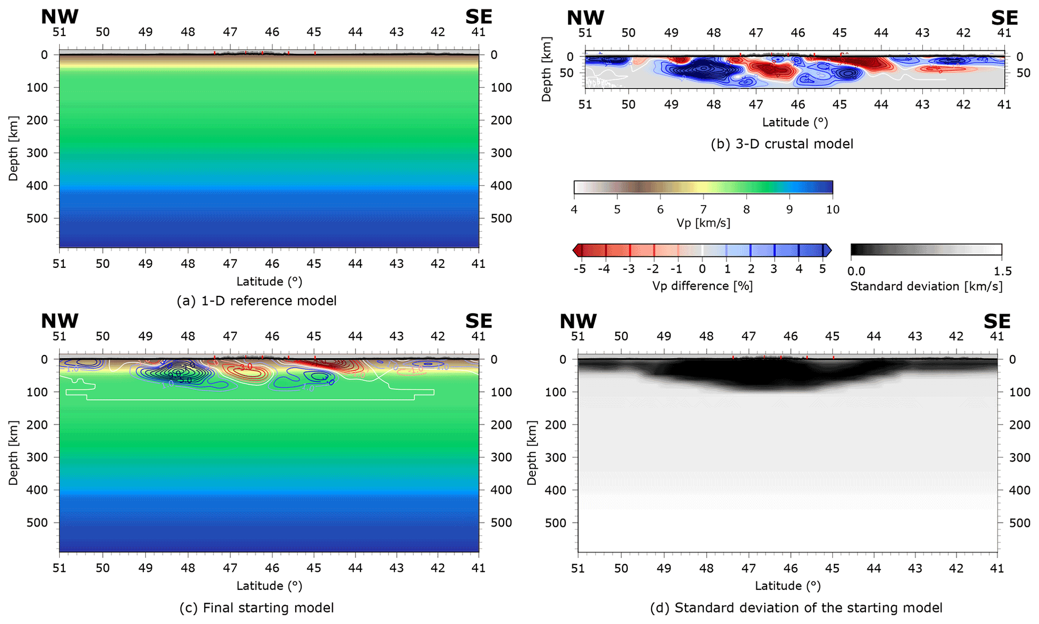
Figure A1(a) We start of from a generic 1D reference model, typically used as a starting model for a seismic tomography, in this case our combined global standard earth model AK135 (Kennett et al., 1995), refined for the Alpine region by using the 1D reference model for the Alpine crust used by Diehl et al. (2009) (Fig. 4). (b) In the next step we superpose the perturbations of our newly calculated 3D crustal model (Sect. 2.4) onto our 1D starting model. The resulting 3D model (c) is then used as starting model for the teleseismic tomography. To control the possible alteration of this starting model during the iterative inversion process, we define an a priori variance for each velocity grid point (d). A variance of 0 (black colour) means that the a priori model remains unchanged during the inversion (e.g. in the uppermost 60 km of the crust below the central Alps), where the resolution of the crustal model is best. As the uncertainty in the crustal model velocities increases, the variance also increases (grey colours), so changes can be made during the inversion if required by the teleseismic data. For the upper mantle outside the resolvable domain of the 3D a priori model for crust and uppermost mantle, we set the a priori variance to 15 % of the model reference velocity (light grey to white colours).
We provide here a small example using Profile P2 from 51.0° N, 6.0° E to 41.0° N, 14.3° E to display how the integration of the crustal model works (Fig. A1).
The tomographic model is available at https://doi.org/10.5880/fidgeo.2021.032 (last access: 2 November 2021, Paffrath and Friederich, 2021). The pick dataset is not publicly available. Please contact the authors for access.
The supplement related to this article is available online at https://doi.org/10.5194/se-12-2671-2021-supplement.
The AlpArray Seismic Network team: György Hetényi, Rafael Abreu, Ivo Allegretti, Maria-Theresia Apoloner, Coralie Aubert, Simon Besançon, Maxime Bès de Berc, Götz Bokelmann, Didier Brunel, Marco Capello, Martina Čarman, Adriano Cavaliere, Jérôme Chèze, Claudio Chiarabba, John Clinton, Glenn Cougoulat, Wayne C. Crawford, Luigia Cristiano, Tibor Czifra, Ezio D’Alema, Stefania Danesi, Romuald Daniel, Anke Dannowski, Iva Dasović, Anne Deschamps, Jean-Xavier Dessa, Cécile Doubre, Sven Egdorf, ETHZ-SED Electronics Lab, Tomislav Fiket, Kasper Fischer, Florian Fuchs, Sigward Funke, Domenico Giardini, Aladino Govoni, Zoltán Gráczer, Gidera Gröschl, Stefan Heimers, Ben Heit, Davorka Herak, Marijan Herak, Johann Huber, Dejan Jarić, Petr Jedlička, Yan Jia, Hélène Jund, Edi Kissling, Stefan Klingen, Bernhard Klotz, Petr Kolínský, Heidrun Kopp, Michael Korn, Josef Kotek, Lothar Kühne, Krešo Kuk, Dietrich Lange, Jürgen Loos, Sara Lovati, Deny Malengros, Lucia Margheriti, Christophe Maron, Xavier Martin, Marco Massa, Francesco Mazzarini, Thomas Meier, Laurent Métral, Irene Molinari, Milena Moretti, Anna Nardi, Jurij Pahor, Anne Paul, Catherine Péquegnat, Daniel Petersen, Damiano Pesaresi, Davide Piccinini, Claudia Piromallo, Thomas Plenefisch, Jaroslava Plomerová, Silvia Pondrelli, Snježan Prevolnik, Roman Racine, Marc Régnier, Miriam Reiss, Joachim ritter, Georg Rümpker, Simone Salimbeni, Marco Santulin, Werner Scherer, Sven Schippkus, Detlef Schulte-Kortnack, Vesna Šipka, Stefano Solarino, Daniele Spallarossa, Kathrin Spieker, Josip Stipčević, Angelo Strollo, Bálint Süle, Gyöngyvér Szanyi, Eszter Szűcs, Christine Thomas, Martin THORWART, Frederik TILMANN, Stefan Ueding, Massimiliano Vallocchia, Luděk Vecsey, René Voigt, Joachim Wassermann, Zoltán Wéber, Christian Weidle, Viktor Wesztergom, Gauthier Weyland, Stefan Wiemer, Felix Wolf, David Wolyniec, Thomas Zieke, Mladen Živčić, Helena Žlebčíková. The Swath-D Working Group: Ben Heit, Michael Weber, Christian Haberland, Frederik Tilmann (Helmholtz-Zentrum Potsdam Deutsches GeoForschungsZentrum [GFZ]) and the Swath-D Field Team: Luigia Cristiano, Peter Pilz, Camilla Cattania, Francesco Maccaferri, Angelo Strollo, Susanne Hemmleb, Stefan Mroczek, Thomas Zieke, Günter Asch, Peter Wigger, James Mechie, Karl Otto, Patricia Ritter, Djamil Al-Halbouni, Alexandra Mauerberger, Ariane Siebert, Leonard Grabow, Xiaohui Yuan, Christoph Sens-Schonfelder, Jennifer Dreiling, Rob Green, Lorenzo Mantiloni, Jennifer Jenkins, Alexander Jordan, Azam Jozi Najafabadi, Susanne Kallenbach (Helmholtz-Zentrum Potsdam Deutsches GeoForschungsZentrum [GFZ]), Ludwig Kuhn, Florian Dorgerloh, Stefan Mauerberger, Jan Seidemann (Universität Potsdam), Rens Hofman (Freie Universität Berlin), Helmut Hausmann, Nikolaus Horn, Stefan Weginger, Anton Vogelmann (Austria: Zentralanstalt für Meteorologie und Geodynamik [ZAMG]), Simone Kasemann (Universität Bremen), Claudio Carraro, Corrado Morelli (Südtirol/Bozen: Amt für Geologie und Baustoffprüfung), Günther Walcher, Martin Pernter, Markus Rauch (Civil Protection Bozen), Giorgio Duri, Michele Bertoni, Paolo Fabris (Istituto Nazionale di Oceanografia e di Geofisica Sperimentale [OGS] [CRS Udine]), Andrea Franceschini, Mauro Zambotto, Luca Froner, Marco Garbin (also OGS) (Ufficio Studi Sismici e Geotecnici-Trento).
WF developed the initial idea of the project. MP developed the code, compiled the dataset and ran the calculations. MP and WF prepared the article. MH and SS assisted with background information on the geology of the Alps and provided interpretations of the horizontal and vertical sections in Chapt. 6.
The contact author has declared that neither they nor their co-authors have any competing interests.
Publisher’s note: Copernicus Publications remains neutral with regard to jurisdictional claims in published maps and institutional affiliations.
This article is part of the special issue “New insights into the tectonic evolution of the Alps and the adjacent orogens”. It is not associated with a conference.
We greatly acknowledge the contributions of the AlpArray temporary network Z3 (Hetényi et al., 2018) and AlpArray Working Group (2015) for making this work possible. We want to thank the Deutsche Forschungsgemeinschaft (DFG) for funding the work within the framework of DFG Priority Programme “Mountain Building Processes in Four Dimensions (MB-4D)” (SPP 2017, grants FR 1146/9-1 and FR 1146/12-1). Many thanks to Tobias Diehl and Liang Zhao for giving us access to their tomographic models. We are very grateful for the comments and contributions of the editor and anonymous reviewers, who put much effort into the revision process to improve the quality of this paper. We want to acknowledge all permanent and other temporary seismic networks used in this study: Malet et al. (2015); Department Of Earth And Environmental Sciences, Geophysical Observatory, University Of München (2001); CERN (2017); Swiss Seismological Service (SED) At ETH Zurich (1983); University Of Zagreb (2001); Institute Of Geophysics, Academy Of Sciences Of The Czech Republic (1973); RESIF (1995); Institut De Physique Du Globe De Paris (IPGP) and Ecole Et Observatoire Des Sciences De La Terre De Strasbourg (EOST) (1982); GEOFON Data Centre (1993); Federal Institute for Geosciences and Natural Resources (1976); University Of Genova (1967); Kövesligethy Radó Seismological Observatory (Geodetic And Geophysical Institute, Research Centre For Astronomy And Earth Sciences, Hungarian Academy Of Sciences (MTA CSFK GGI KRSZO)) (1992); Albuquerque Seismological Laboratory (ASL)/USGS (1988); INGV Seismological Data Centre (1997); MedNet Project Partner Institutions (1988); French Landslide Observatory – Seismological Datacenter/RESIF (2006); OGS (Istituto Nazionale Di Oceanografia E Di Geofisica Sperimentale) And University Of Trieste (2002); ZAMG – Zentralanstalt Für Meterologie Und Geodynamik (1987); OGS (Istituto Nazionale Di Oceanografia E Di Geofisica Sperimentale) (2016); Polish Academy of Sciences (PAN) Polskiej Akademii Nauk (1990); RESIF (2018); University Of Trieste (1993); ZAMG - Central Institute for Meteorology and Geodynamics (2006); ESI SAS (Earth Science Institute Of The Slovak Academy Of Sciences) (2004); Slovenian Environment Agency (2001); Geological Survey-Provincia Autonoma Di Trento (1981); Leipzig University (2001); Jena (2009); McKee et al. (2018); Guéguen et al. (2017); Deschamps and Beucler (2013). The authors would also like to thank all members of the AlpArray Seismic Network team and the AlpArray SWATH-D working group and field team, mentioned in the team list above. As well as the members of the EASI field team: Jaroslava Plomerová, Helena Munzarová, Ludek Vecsey, Petr Jedlicka, Josef Kotek, Irene Bianchi, Maria-Theresia Apoloner, Florian Fuchs, Patrick Ott, Ehsan Qorbani, Katalin Gribovszki, Peter Kolinsky, Peter Jordakiev, Hans Huber, Stefano Solarino, Aladino Govoni, Simone Salimbeni, Lucia Margheriti, Adriano Cavaliere, John Clinton, Roman Racine, Sacha Barman, Robert Tanner, Pascal Graf, Laura Ermert, Anne Obermann, Stefan Hiemer, Meysam Rezaeifar, Edith Korger, Ludwig Auer, Korbinian Sager, György Hetényi, Irene Molinari, Marcus Herrmann, Saulé Zukauskaité, Paula Koelemeijer, Sascha Winterberg. For more information on the team visit http://www.alparray.ethz.ch/en/home/. A special thanks to the authors of Matplotlib (Hunter, 2007) for providing a powerful toolkit for scientific data and map visualization with the help of Basemap. Many thanks to GFZ Data Services for providing a platform to share our model results. Last but not least we want to thank the seismology group of the Ruhr-Universität Bochum, which helped to improve the quality of this work by numerous discussions and contributions.
This research has been supported by the Deutsche Forschungsgemeinschaft (grant nos. FR 1146/9-1 and FR 1146/12-1).
This paper was edited by Anne Paul and reviewed by two anonymous referees.
Aki, K., Christoffersson, A., and Husebye, E. S.: Determination of the three-dimensional seismic structure of the lithosphere, J. Geophys. Res., (1896-1977), 82, 277–296, https://doi.org/10.1029/JB082i002p00277, 1977. a
Albuquerque Seismological Laboratory (ASL)/USGS: Global Seismograph Network (GSN – IRIS/USGS), https://doi.org/10.7914/SN/IU, 1988. a
AlpArray Working Group: AlpArray Seismic Network (AASN) temporary component, https://doi.org/10.12686/ALPARRAY/Z3_2015, 2015. a
Babuška, V., PlomerovÁ, J., and Granet, M.: The deep lithosphere in the Alps: a model inferred from P residuals, Tectonophysics, 176, 137–165, https://doi.org/10.1016/0040-1951(90)90263-8, 1990. a
Barruol, G., Bonnin, M., Pedersen, H., Bokelmann, G. H., and Tiberi, C.: Belt-parallel mantle flow beneath a halted continental collision: The Western Alps, Earth Planet. Sci. Letters, 302, 429–438, 2011. a, b
Bezada, M. J., Faccenda, M., and Toomey, D. R.: Representing anisotropic subduction zones with isotropic velocity models: A characterization of the problem and some steps on a possible path forward, Geochem. Geophys. Geosys., 17, 3164–3189, https://doi.org/10.1002/2016gc006507, 2016. a, b
Blundell, D. J., Freeman, R., Mueller, S., and Button, S.: A continent revealed: The European Geotraverse, structure and dynamic evolution, Cambridge University Press, 1992. a
Boschi, L., Fry, B., Ekström, G., and Giardini, D.: The European upper mantle as seen by surface waves, Surv. Geophys., 30, 463–501, 2009. a
CERN: CERN Seismic Network, available at: https://www.fdsn.org/networks/detail/C4/ (last access: 3 September 2021), 2017. a
Crotwell, H., Owens, T., and Ritsema, J.: The TauP Toolkit: Flexible Seismic Travel-Time and Raypath Utilities, Seismological Research Letters, 70, https://doi.org/10.1785/gssrl.70.2.154, 1999. a
Department Of Earth And Environmental Sciences, Geophysical Observatory, University Of München: BayernNetz, https://doi.org/10.7914/SN/BW, 2001. a
Deschamps, A. and Beucler, E.: POSA experiment, https://doi.org/10.15778/RESIF.ZH2016, 2013. a
Diehl, T., Husen, S., Kissling, E., and Deichmann, N.: High-resolution 3D P-wave model of the Alpine crust, Geophys. J. Int., 179, 1133–1147, https://doi.org/10.1111/j.1365-246X.2009.04331.x, 2009. a, b, c, d, e, f, g, h
Dziewonski, A. M., Chou, T.-A., and Woodhouse, J. H.: Determination of earthquake source parameters from waveform data for studies of global and regional seismicity, J. Geophys. Res.-Sol. Ea., 86, 2825–2852, https://doi.org/10.1029/JB086iB04p02825, 1981. a
EASI: Eastern Alpine Seismic Investigation, https://doi.org/10.12686/alparray/xt_2014, 2014. a, b
Ekström, G., Nettles, M., and Dziewonski, A.: The global CMT project 2004-2010: Centroid-moment tensors for 13,017 earthquakes, Phys. Earth Planet. Int., 200, 1–9, https://doi.org/10.1016/j.pepi.2012.04.002, 2012. a
El-Sharkawy, A., Meier, T., Lebedev, S., Behrmann, J. H., Hamada, M., Cristiano, L., Weidel, C., and Köhn, D.: The slab puzzle of the Alpine‐Mediterranean region: Insights from a new, high‐resolution, shear wave velocity model of the upper mantle, Geochem. Geophys. Geosys., 21, e2020GC008993, https://doi.org/10.1029/2020GC008993, 2020. a
ESI SAS (Earth Science Institute Of The Slovak Academy Of Sciences): National Network of Seismic Stations of Slovakia, https://doi.org/10.14470/FX099882, 2004. a
Federal Institute for Geosciences and Natural Resources: German Regional Seismic Network (GRSN), https://doi.org/10.25928/MBX6-HR74, 1976. a
Frei, W., Hertzmann, P., Lehner, P., Olivier, R., Pfiffner, A., Steck, A., and Valasek, P.: Geotraverses across the Swiss Alps, Nature, 340, 544–548, 1989. a
French Landslide Observatory – Seismological Datacenter/RESIF: Observatoire Multi-disciplinaire des Instabilités de Versants (OMIV), https://doi.org/10.15778/RESIF.MT, 2006. a
Fry, B., Deschamps, F., Kissling, E., Stehly, L., and Giardini, D.: Layered azimuthal anisotropy of Rayleigh wave phase velocities in the European Alpine lithosphere inferred from ambient noise, Earth Planet. Sci. Lett., 297, 95–102, 2010. a
GEOFON Data Centre: GEOFON Seismic Network, https://doi.org/10.14470/TR560404, 1993. a
Geological Survey-Provincia Autonoma Di Trento: Trentino Seismic Network, https://doi.org/10.7914/SN/ST, 1981. a
Giacomuzzi, G., Chiarabba, C., and De Gori, P.: Linking the Alps and Apennines subduction systems: New constraints revealed by high-resolution teleseismic tomography, Earth Planet. Sci. Lett., 301, 531–543, 2011. a
Guéguen, P., Coutant, O., Langlais, M., and RESIF: Maurienne Seismic Swarm 2017-2018, https://doi.org/10.15778/RESIF.YW2017, 2017. a
Handy, M. R., Schmid, S. M., Bousquet, R., Kissling, E., and Bernoulli, D.: Reconciling plate-tectonic reconstructions of Alpine Tethys with the geological–geophysical record of spreading and subduction in the Alps, Earth-Sci. Rev., 102, 121–158, https://doi.org/10.1016/j.earscirev.2010.06.002, 2010. a
Handy, M. R., Ustaszewski, K., and Kissling, E.: Reconstructing the Alps–Carpathians–Dinarides as a key to understanding switches in subduction polarity, slab gaps and surface motion, Int. J. Earth Sci., 104, 1–26, https://doi.org/10.1007/s00531-014-1060-3, 2014. a
Handy, M., Schmid, S., Paffrath, M., Friederich, W., and the AlpArray Working Group: Orogenic lithosphere and slabs in the greater Alpine area – interpretations based on teleseismic P-wave tomography, Solid Earth, 12, 2633–2669, https://doi.org/10.5194/se-12-2633-2021, 2021. a, b, c, d, e, f, g, h, i, j, k
Heit, B., Weber, M., Tilmann, F., Haberland, C., Jia, Y., Carraro, C., Walcher, G., Franceschini, A., and Pesaresi, D.: The Swath-D Seismic Network in Italy and Austria, https://doi.org/10.14470/MF7562601148, 2017. a, b
Hetényi, G., Molinari, I., Clinton, J., et al.: The AlpArray Seismic Network: A Large-Scale European Experiment to Image the Alpine Orogen, Surv. Geophys., 39, 1009–1033, https://doi.org/10.1007/s10712-018-9472-4, 2018. a, b, c
Hirn, A., Nadir, S., Thouvenot, F., Nicolich, R., Pellis, G., Scarascia, S., Tabacco, I., Castellano, F., and Merlanti, F.: Mapping the Moho of the Western Alps by wide-angle reflection seismics, Tectonophysics, 162, 193–202, https://doi.org/10.1016/0040-1951(89)90243-6, 1989. a
Hunter, J. D.: Matplotlib: A 2D graphics environment, Comput. Sci. Eng., 9, 90–95, https://doi.org/10.1109/MCSE.2007.55, 2007. a
INGV Seismological Data Centre: Rete Sismica Nazionale (RSN), https://doi.org/10.13127/SD/X0FXNH7QFY, 1997. a
Institut De Physique Du Globe De Paris (IPGP) and Ecole Et Observatoire Des Sciences De La Terre De Strasbourg (EOST): GEOSCOPE, French Global Network of broad band seismic stations, https://doi.org/10.18715/GEOSCOPE.G, 1982. a
Institute Of Geophysics, Academy Of Sciences Of The Czech Republic: Czech Regional Seismic Network, https://doi.org/10.7914/SN/CZ, 1973. a
Jena, F. S. U.: Thüringer Seismologisches Netz (TSN), https://doi.org/10.7914/SN/TH, 2009. a
Jolivet, L. and Facenna, C.: Mediterranean extension and Africa-Eurasia collision, Tectonics, 19, 1095–1106, 2000. a, b
Karousova, H., Plomerova, J., and Babuska, V.: Upper-mantle structure beneath the southern Bohemian Massif and its surroundings imaged by high-resolution tomography, Geophys. J. Int., 194, 1203–1215, https://doi.org/10.1093/gji/ggt159, 2013. a
Kennett, B. L. N., Engdahl, E. R., and Buland, R.: Constraints on seismic velocities in the Earth from traveltimes, Geophys. J. Int., 122, 108–124, https://doi.org/10.1111/j.1365-246X.1995.tb03540.x, 1995. a, b
Kissling, E.: Deep structure of the Alps – what do we really know?, Phys. Earth Planet. Int., 79, 87–112, https://doi.org/10.1016/0031-9201(93)90144-X, 1993. a
Kissling, E., Schmid, S., and Ansorge, J.: Lithosphere structure and tectonic evolution of the Alpine arc: New evidence from high-resolution teleseismic tomography, Geological Society London Memoirs, 32, https://doi.org/10.1144/GSL.MEM.2006.032.01.08, 2006. a
Koulakov, I., Kaban, M. K., Tesauro, M., and Cloetingh, S.: P- and S-velocity anomalies in the upper mantle beneath Europe from tomographic inversion of ISC data, Geophys. J. Int., 179, 345–366, https://doi.org/10.1111/j.1365-246X.2009.04279.x, 2009. a, b, c, d, e, f, g
Krischer, L., Megies, T., Barsch, R., Beyreuther, M., Lecocq, T., Caudron, C., and Wassermann, J.: ObsPy: A bridge for seismology into the scientific Python ecosystem, Comput. Sci. Discov., 8, 014003, https://doi.org/10.1088/1749-4699/8/1/014003, 2015. a
Kummerow, J., Kind, R., Oncken, O., Giese, P., Ryberg, T., Wylegalla, K., Scherbaum, F., Transalp Working Group, et al.: A natural and controlled source seismic profile through the Eastern Alps: TRANSALP, Earth Planet. Sci. Lett., 225, 115–129, 2004. a
Kästle, E. D., El-Sharkawy, A., Boschi, L., Meier, T., Rosenberg, C., Bellahsen, N., Cristiano, L., and Weidle, C.: Surface wave tomography of the Alps using ambient-noise and earthquake phase velocity measurements, J. Geophys. Res.-Sol. Ea., 123, 1770–1792, https://doi.org/10.1002/2017JB014698, 2018. a
Kästle, E. D., Rosenberg, C., Boschi, L., Bellahsen, N., Meier, T., and El-Sharkawy, A.: Slab break-offs in the Alpine subduction zone, International J. Earth Sci., 109, 587–603, https://doi.org/10.1007/s00531-020-01821-z, 2020. a, b, c
Kövesligethy Radó Seismological Observatory (Geodetic And Geophysical Institute, Research Centre For Astronomy And Earth Sciences, Hungarian Academy Of Sciences (MTA CSFK GGI KRSZO)): Hungarian National Seismological Network, https://doi.org/10.14470/UH028726, 1992. a
Küperkoch, L., Meier, T., Lee, J., Friederich, W., and the EGELADOS Working Group: Automated determination of P-phase arrival times at regional and local distances using higher order statistics, Geophysical Journal International, 181, 1159–1170, https://doi.org/10.1111/j.1365-246X.2010.04570.x, 2010. a
Legendre, C., Meier, T., Lebedev, S., Friederich, W., and Viereck-Götte, L.: A shear wave velocity model of the European upper mantle from automated inversion of seismic shear and surface waveforms, Geophys. J. Int., 191, 282–304, 2012. a
Leipzig University: SXNET Saxon Seismic Network, https://doi.org/10.7914/SN/SX, 2001. a
Link, F. and Rümpker, G.: The mantle flow below the Alps from isolated mantle anisotropy based on differential Ps – XKS Splitting, in: EGU General Assembly Conference Abstracts, EGU General Assembly Conference Abstracts, p. 2810, 2020. a
Lippitsch, R., Kissling, E., and Ansorge, J.: Upper mantle structure beneath the Alpine orogen from high-resolution teleseismic tomography, J. Geophys. Res., 108, https://doi.org/10.1029/2002JB002016, 2003. a, b, c, d, e, f, g, h, i, j, k, l, m, n
Lombardi, D., Braunmiller, J., Kissling, E., and Giardini, D.: Moho depth and Poisson's ratio in the Western-Central Alps from receiver functions, Geophys. J. Int., 173, 249–264, 2008. a
Lombardi, D., Braunmiller, J., Kissling, E., and Giardini, D.: Alpine mantle transition zone imaged by receiver functions, Earth Planet. Sci. Lett., 278, 163–174, 2009. a
Luth, S., Willingshofer, E., Sokoutis, D., and Cloetingh, S.: Does subduction polarity change below the Alps? Inferences from analogue modelling, Tectonophysics, 582, 140–161, 2013. a
Malet, J.-P., Hibert, C., Radiguet, M., Gautier, S., Larose, E., Amitrano, D., Jongmans, D., Bièvre, G., and RESIF: French Landslide Observatory – OMIV (Temporary data) (MT-campagne) (RESIF – SISMOB), https://doi.org/10.15778/RESIF.1N2015, 2015. a
Marone, F., Van Der Lee, S., and Giardini, D.: Three-dimensional upper-mantle S-velocity model for the Eurasia–Africa plate boundary region, Geophys. J. Int., 158, 109–130, 2004. a
McKee, K. F., Roman, D., Fee, D., Ripepe, M., AIUPPA, A., and Waite, G.: Seismo-acoustic Network at Stromboli Volcano, Italy, https://doi.org/10.7914/SN/YI_2018, 2018. a
MedNet Project Partner Institutions: Mediterranean Very Broadband Seismographic Network (MedNet), https://doi.org/10.13127/SD/FBBBTDTD6Q, 1988. a
Mitterbauer, U., Behm, M., Brückl, E., Lippitsch, R., Guterch, A., Keller, G. R., Koslovskaya, E., Rumpfhuber, E.-M., and Šumanovac, F.: Shape and origin of the East-Alpine slab constrained by the ALPASS teleseismic model, Tectonophysics, 510, 195–206, https://doi.org/10.1016/j.tecto.2011.07.001, 2011. a, b, c, d, e, f, g, h, i
Molinari, I., Verbeke, J., Boschi, L., Kissling, E., and Morelli, A.: Italian and Alpine three-dimensional crustal structure imaged by ambient-noise surface-wave dispersion, Geochem. Geophys. Geosyst, 16, 4405–4421, https://doi.org/10.1002/2015GC006176, 2015. a
Mueller, S. and Banda, E.: European geotraverse project, Terra cognita, 3, 291–294, 1983. a
OGS (Istituto Nazionale Di Oceanografia E Di Geofisica Sperimentale): North-East Italy Seismic Network, https://doi.org/10.7914/SN/OX, 2016. a
OGS (Istituto Nazionale Di Oceanografia E Di Geofisica Sperimentale) And University Of Trieste: North-East Italy Broadband Network, https://doi.org/10.7914/SN/NI, 2002. a
Paffrath, M. and Friederich, W.: P-wave traveltime tomography model derived from AlpArray Seismic Network data, GFZ Data Services [data set], https://doi.org/10.5880/fidgeo.2021.032, last access: 2 November 2021. a, b
Paffrath, M., Friederich, W., and the AlpArray and AlpArray-SWATH D Working Groups: Teleseismic P waves at the AlpArray seismic network: wave fronts, absolute travel times and travel-time residuals, Solid Earth, 12, 1635–1660, https://doi.org/10.5194/se-12-1635-2021, 2021a. a, b, c, d, e
Peter, D., Boschi, L., Deschamps, F., Fry, B., Ekström, G., and Giardini, D.: A new finite-frequency shear-velocity model of the European-Mediterranean region, Geophys. Res. Lett., 35, 16, https://doi.org/10.1029/2008gl034769, 2008. a
Pfiffner, O.-A., Frei, W., Finckh, P., and Valasek, P.: Deep seismic reflection profiling in the Swiss Alps: explosion seismology results for line NFP 20-East, Geology, 16, 987–990, 1988. a
Piromallo, C. and Morelli, A.: P wave tomography of the mantle under the Alpine-Mediterranean area, J. Geophys. Res.-Sol. Ea., 108, 2065, https://doi.org/10.1029/2002JB001757, 2003. a, b
Polish Academy of Sciences (PAN) Polskiej Akademii Nauk: Polish Seismological Network, available at: https://www.igf.edu.pl/stacje-en.php (last access: 3 September 2021), 1990. a
Rawlinson, N. and Sambridge, M.: The fast marching method: An effective tool for tomographic imaging and tracking multiple phases in complex layered media, Explor. Geophys., 36, 4, https://doi.org/10.1071/EG05341, 2005. a, b
Rawlinson, N., Reading, A. M., and Kennett, B. L.: Lithospheric structure of Tasmania from a novel form of teleseismic tomography, J. Geophys. Res.-Sol. Ea., 111, B2, https://doi.org/10.1029/2005jb003803, 2006. a
RESIF: RESIF-RLBP French Broad-band network, RESIF-RAP strong motion network and other seismic stations in metropolitan France, https://doi.org/10.15778/RESIF.FR, 1995. a
RESIF: CEA/DASE broad-band permanent network in metropolitan France, https://doi.org/10.15778/RESIF.RD, 2018. a
Schmid, C., van der Lee, S., VanDecar, J., Engdahl, E., and Giardini, D.: Three-dimensional S velocity of the mantle in the Africa-Eurasia plate boundary region from phase arrival times and regional waveforms, J. Geophys. Res., 113, B033306, https://doi.org/10.1029/2005JB004193, 2008. a
Schmid, S., Fügenschuh, B., Kissling, E., and Schuster, R.: Tectonic map and overall architecture of the Alpine orogen, Eclogae Geol. Helv, 97, 93–117, 2004. a
Schmid, S. M., Kissling, E., Diehl, T., Hinsbergen, D. J. J., and Molli, G.: Ivrea mantle wedge, arc of the Western Alps, and kinematic evolution of the Alps–Apennines orogenic system, Swiss J. Geosci., 110, 581–612, https://doi.org/10.1007/s00015-016-0237-0, 2017. a
Slovenian Environment Agency: Seismic Network of the Republic of Slovenia, https://doi.org/10.7914/SN/SL, 2001. a
Spada, M., Bianchi, I., Kissling, E., Agostinetti, N. P., and Wiemer, S.: Combining controlled-source seismology and receiver function information to derive 3D Moho topography for Italy, Geophys. J. Int., 194, 1050–1068, https://doi.org/10.1093/gji/ggt148, 2013. a, b, c
Spakman, W., van der Lee, S., and van der Hilst, R.: Travel-time tomography of the European-Mediterranean mantle down to 1400 km, Phys. Earth Planet. Int., 79, 3–74, 1993. a, b
Stehly, L., Fry, B., Campillo, M., Shapiro, N. M., Guilbert, J., Boschi, L., and Giardini, D.: Tomography of the Alpine region from observations of seismic ambient noise, Geophys. J. Int., 178, 338–350, https://doi.org/10.1111/j.1365-246x.2009.04132.x, 2009. a
Swiss Seismological Service (SED) At ETH Zurich: National Seismic Networks of Switzerland, https://doi.org/10.12686/SED/NETWORKS/CH, 1983. a
Tesauro, M., Kaban, M. K., and Cloetingh, S. A. P. L.: EuCRUST-07: A new reference model for the European crust, Geophys. Res. Lett., 35, 5, https://doi.org/10.1029/2007GL032244, 2008. a, b, c, d
TRANSALP Working Group, Gebrande, H., Lüschen, E., Bopp, M., Bleibinhaus, F., Lammerer, B., Oncken, O., Stiller, M., Kummerow, J., Kind, R., et al.: First deep seismic reflection images of the Eastern Alps reveal giant crustal wedges and transcrustal ramps, Geophys. Res. Lett., 29, https://doi.org/10.1029/2001GL014911, 2002. a
University Of Genova: Regional Seismic Network of North Western Italy, https://doi.org/10.7914/SN/GU, 1967. a
University Of Trieste: Friuli Venezia Giulia Accelerometric Network, https://doi.org/10.7914/SN/RF, 1993. a
University Of Zagreb: Croatian Seismograph Network, https://doi.org/10.7914/SN/CR, 2001. a
Waldhauser, F., Lippitsch, R., Kissling, E., and Ansorge, J.: High-resolution teleseismic tomography of upper-mantle structure using an a priori three-dimensional crustal model, Geophys. J. Int., 150, 403–414, https://doi.org/10.1046/j.1365-246X.2002.01690.x, 2002. a
ZAMG – Central Institute for Meteorology and Geodynamics: Province Südtirol, available at: https://www.fdsn.org/networks/detail/SI/ (last access: 3 September 2021), 2006. a
ZAMG – Zentralanstalt Für Meterologie Und Geodynamik: Austrian Seismic Network, https://doi.org/10.7914/SN/OE, 1987. a
Zhao, L., Paul, A., Malusà, M. G., Xu, X., Zheng, T., Solarino, S., Guillot, S., Schwartz, S., Dumont, T., Salimbeni, S., Aubert, C., Pondrelli, S., Wang, Q., and Zhu, R.: Continuity of the Alpine slab unraveled by high-resolution P wave tomography, J. Geophys. Res.-Sol. Ea., 121, 8720–8737, https://doi.org/10.1002/2016JB013310, 2016. a, b, c, d, e, f, g, h, i, j, k
Zhu, H., Bozdağ, E., Peter, D., and Tromp, J.: Structure of the European upper mantle revealed by adjoint tomography, Nat. Geosci., 5, 493–498, https://doi.org/10.1038/ngeo1501, 2012. a
- Abstract
- Introduction
- Methods
- Data basis
- Resolution analysis
- Results
- Discussion
- Conclusions
- Appendix A: Crustal model integration
- Data availability
- Team list
- Author contributions
- Competing interests
- Disclaimer
- Special issue statement
- Acknowledgements
- Financial support
- Review statement
- References
- Supplement
- Article
(48449 KB) - Full-text XML
- Abstract
- Introduction
- Methods
- Data basis
- Resolution analysis
- Results
- Discussion
- Conclusions
- Appendix A: Crustal model integration
- Data availability
- Team list
- Author contributions
- Competing interests
- Disclaimer
- Special issue statement
- Acknowledgements
- Financial support
- Review statement
- References
- Supplement