the Creative Commons Attribution 4.0 License.
the Creative Commons Attribution 4.0 License.
 | 29 Jun 2022
The analysis of slip tendency of major tectonic faults in Germany
Steffen Ahlers
Birgit Müller
Karsten Reiter
Oliver Heidbach
Andreas Henk
Tobias Hergert
Frank Schilling
Seismic hazard during subsurface operations is often related to the reactivation of pre-existing tectonic faults. The analysis of the slip tendency, i.e., the ratio of shear to normal stress acting on the fault plane, allows an assessment of the reactivation potential of faults. We use the total stresses that result from a large-scale 3D geomechanical–numerical model of Germany and adjacent areas to calculate the slip tendency for three 3D fault geometry sets with increasing complexity. This allows us to draw general conclusions about the influence of the fault geometry on the reactivation potential.
In general, the fault reactivation potential is higher in Germany for faults that strike NW–SE and NNE–SSW. Due to the prevailing normal stress regime in the geomechanical–numerical model results, faults dipping at an angle of about 60∘ generally show higher slip tendencies in comparison to steeper or shallower dipping faults. Faults implemented with a straight geometry show higher slip tendencies than those represented with a more complex, uneven geometry. Pore pressure has been assumed to be hydrostatic and has been shown to have a major influence on the calculated slip tendencies. Compared to slip tendency values calculated without pore pressure, the consideration of pore pressure leads to an increase in slip tendency of up to 50 %. The qualitative comparison of the slip tendency with the occurrence of seismic events with moment magnitudes Mw>3.5 shows areas with an overall good spatial correlation between elevated slip tendencies and seismic activity but also highlights areas where more detailed and diverse fault sets would be beneficial.
Please read the corrigendum first before continuing.
-
Notice on corrigendum
The requested paper has a corresponding corrigendum published. Please read the corrigendum first before downloading the article.
-
Article
(7256 KB)
- Corrigendum
-
Supplement
(2089 KB)
-
The requested paper has a corresponding corrigendum published. Please read the corrigendum first before downloading the article.
- Article
(7256 KB) - Full-text XML
- Corrigendum
-
Supplement
(2089 KB) - BibTeX
- EndNote


Seismic activity is a crucial aspect for many subsurface constructions and activities such as the production of oil and gas, coal mining, geothermal energy production, the storage of gas, or the construction and safe long-term operation of a nuclear waste repository. The occurrence of seismic activity is closely linked to the presence of pre-existing tectonic faults and their reactivation (Sibson, 1985). To estimate the potential to trigger seismic events, knowledge about the reactivation potential of tectonic faults is essential (Moeck et al., 2009; Worum et al., 2004). Slip on a fault occurs when the resolved shear stress τ is larger than the frictional resistance τf (Sibson, 1974; Jaeger et al., 2011):
where C is the fault cohesion, μ is the coefficient of static friction and σneff the effective normal stress on the fault. The relevant parameters for the assessment of the fault reactivation potential are therefore the following: (1) the stress tensor to estimate τ and the absolute normal stress σn; (2) the pore pressure required for the calculation of σneff; (3) the fault orientation that influences the magnitudes of σn and τ; (4) the frictional fault properties C and μ that describe the fault's mechanical behavior.
The stress tensor in previous works has mainly been estimated utilizing stress inversion (McFarland et al., 2012; Yukutake et al., 2015; Ferrill et al., 2020), point-wise stress data from field observations (Neves et al., 2009; Lee and Chang, 2009; Moeck et al., 2009; Morris et al., 2021) or Monte Carlo simulation (Healy and Hicks, 2022) for 2D lineaments and in some cases 3D fault geometries. Worum et al. (2004) calculated the 3D stress tensor with an analytical model and used it for the estimation of the fault reactivation potential of 3D faults of the Roer Valley Graben. Stress tensor estimates from 3D geomechanical–numerical models have been used to determine fault reactivation potential on regional scales, e.g., for the Upper Rhine Graben (Peters, 2007) or the Val d'Agri (Italy) (Vadacca et al., 2021), but this has not been achieved for all of Germany. In this study, we focus on the whole of Germany.
Here, we use the first 3D geomechanical–numerical model of Germany by Ahlers et al. (2021b) that provides an estimate of the 3D stress tensor that is variable with depth and lateral extent (Cornet and Röckel, 2012) due to inhomogeneous density and elastic rock properties. Furthermore, we compile three sets of 3D fault geometries with increasing complexity and use the stress tensor from the Germany model to predict the fault reactivation potential. The fault sets can be used not only to derive a first-order estimation of the fault reactivation potential but also to highlight the effect of fault geometry on the fault reactivation potential. We also investigate the impact of hydrostatic pore pressure as well as assumed overpressure on the reactivation potential estimates and compare our results with the spatial distribution of seismic events with moment magnitudes Mw≥3.5.
2.1 Study area
This study focuses on Germany and some adjacent areas. It is subdivided into the three crustal units of the East European Craton, Avalonia and the Amorican Terrane Assemblage (Meschede and Warr, 2019; Ahlers et al., 2021a) (Fig. 1a). Most parts of the European basement have a Variscan overprint and can be subdivided into the roughly SW–NE-striking regions defined by Kossmat: the Rhenohercynican, the Saxothuringian, including the Mid-German Crystalline Zone, and the Moldanubian Zone (Walter, 2007). North Germany is characterized by the North German Basin as part of the Southern Permian Basin (van Wees et al., 2000) and almost N–S-striking graben structures such as the Glückstadt Graben and SW–SE-striking basins (Walter, 2007). Central and south Germany are characterized by several low mountain ranges such as the Black Forest, the Harz, the Ore Mountains or the Rhenish Massif and sedimentary basins such as the Upper Rhine Graben and the Molasse Basin. The southernmost part of Germany is dominated by the roughly E–W-striking Alps.
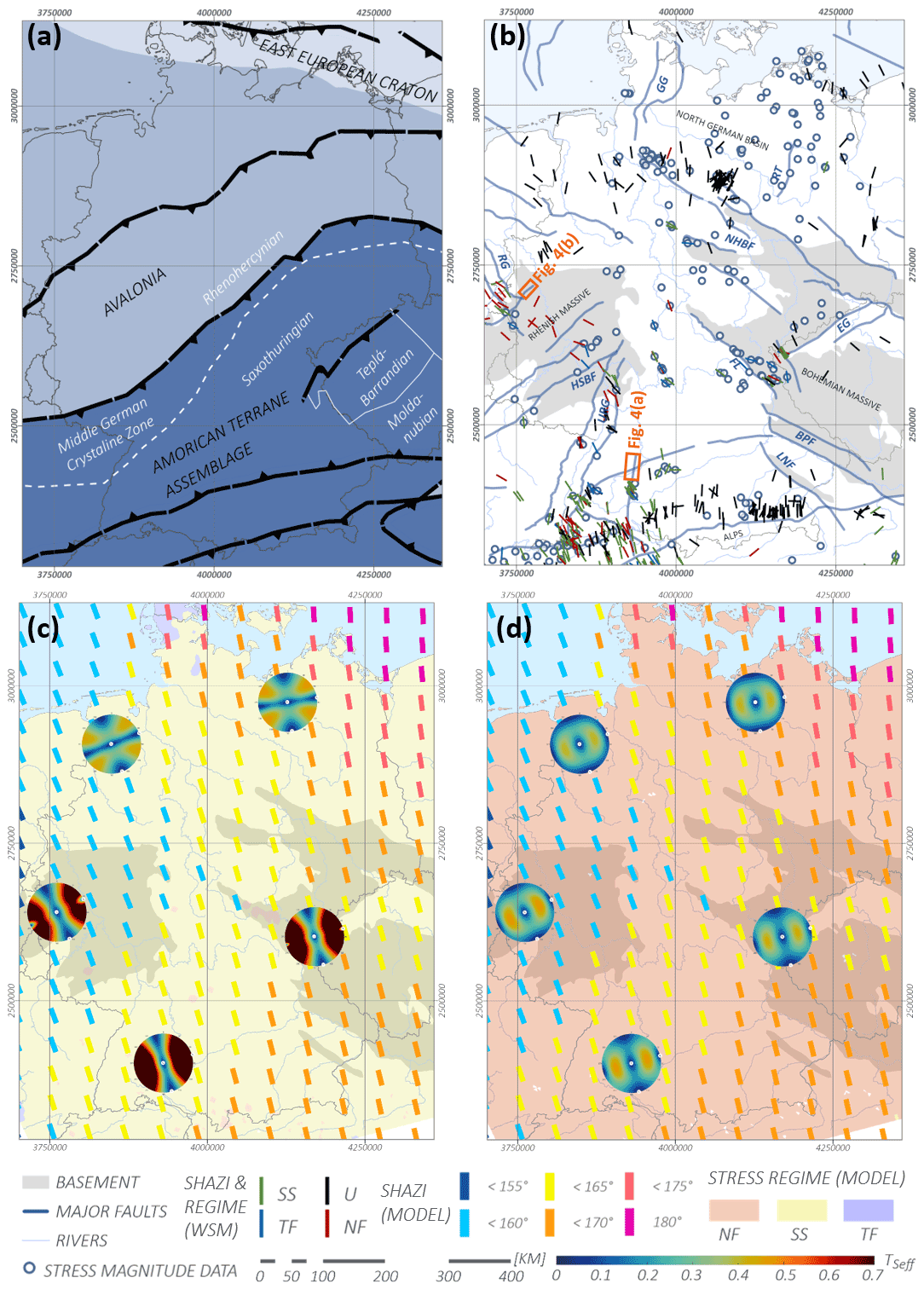
Figure 1(a) Crustal units in Germany are indicated by different shades of blue and labeled with dark gray, capital text. White text labels Variscan units. Modified after Meschede and Warr (2019) and Ahlers et al. (2021a). (b) Stress data available in Germany: the rotated line markers represent data on the orientation of the maximum horizontal stress (SHazi) available in the World Stress Map (Heidbach et al., 2016) and are colored by the stress regime associated with the data points (normal faulting (NF), strike-slip faulting (SS), thrust faulting (TF) and unknown regime (U)). Plotted alongside are the locations of stress magnitude data (Morawietz and Reiter, 2020) and major tectonic faults in Germany as blue lines with (outcropping) basement structures indicated by gray areas The location of Fig. 4a and b is indicated by orange squares. BPF: Bavarian Pfahl Fault; EG: Eger Graben; FL: Franconian Line; GG: Glückstadt Graben; HSBF: Hunsrück Southern Border Fault; LNF: Landshut–Neuötting Fault; NHBF: Northern Harz Boundary fault; RG: Roer Valley Graben: RT: Rheinsberg Trough; URG: Upper Rhine Graben (modified after Kley and Voigt, 2008 and Ahlers et al., 2021a). Panels (c) and (d): the stress regime calculated by the Germany model at 1 and 8 km depth, respectively, is indicated by the background color; SHazi calculated by the Germany model has been averaged along a regular grid. The mean SHazi of each grid point is indicated by the orientation and color of the marker. For five areas within the model area, fault reactivation stereo plots are shown, displaying what fault orientations and dips are most favorable for reactivation under the given stress conditions. ©EuroGeographics for the administrative boundaries.
Seismicity is mainly observed in the Rhine area, the Swabian Jura and eastern Thuringia as well as western Saxony (German Research Centre For Geosciences, 2022). Induced seismicity has mainly been documented in the context of gas production (Müller et al., 2020), geothermal energy production (Bönnemann et al., 2010; Stober and Bucher, 2020) and especially mining activities, which have caused induced seismic events with local magnitudes of up to 5.6 (Grünthal and Minkley, 2005). Poro-elastic stress changes should be considered for significant pore pressure changes, as shown for production-induced earthquakes (Müller et al., 2020). In the case of geothermal sites, fluid injections into the sedimentary rocks have been suggested to not be as seismogenic as injections into crystalline rocks. In general, the presence of faults close to the injection well as fluid pathways increases the risk of seismic events (Evans et al., 2012)
2.2 Stress state
Stress data are not evenly distributed throughout Germany (Fig. 1b) and vary between different regions of Germany both in terms of orientation and the stress magnitudes, i.e., the stress regime. For the North German Basin, Röckel and Lempp (2003) describe a normal faulting regime and mostly N–S-striking SHmax orientations (SHazi) with a NNW–SSE influence towards the Dutch border and an NNE–SSW influence towards Poland. For the Upper Rhine Graben (URG) area in southwest Germany, Homuth et al. (2014) calculate a transtensional regime with a strong strike-slip influence with SHazi around 135∘, while modeling results of Buchmann and Connolly (2007) suggest a present-day strike-slip reactivation of the URG. For the Molasse Basin in south Germany, SHazi rotates from striking N–S in southeast Germany to striking NNW–SSE in the southwest (Reinecker et al., 2010), and the stress regime most likely varies between normal faulting and strike slip (Drews et al., 2019; Seithel et al., 2015)
Since these stress data are available only point-wise, we use the stress tensor derived from the 3D geomechanical–numerical model of Germany by Ahlers et al. (2021b) for the assessment of the fault reactivation potential. The model covers Germany and adjacent areas and provides a continuum-mechanics-based prediction of the stress tensor. The purely elastic finite-element (FE) model comprises seven mechanical units, i.e., sediments, four upper crustal units, the lower crust and parts of the lithospheric mantle. The four crustal units represent the crustal framework of Germany as shown in Fig. 1a and the Alps–Carpathian–Pannonia. The lateral grid resolution is 6 × 6 km2 and the vertical resolution decreases from 800 m within the sediments to 7500 m at the model base. Each unit is characterized by its respective density, Young's modulus and Poisson's ratio (Ahlers et al., 2021a).
The model is calibrated with stress magnitude data from the magnitude database by Morawietz et al. (2020) and compared with stress orientations from the World Stress Map database (Heidbach et al., 2016); both data sets are shown in Fig. 1b. The resulting best-fit model provides the 3D absolute stress tensor σij within the model domain (Ahlers et al., 2021a), i.e., for Germany and adjacent areas. In order to consider effective stresses, we assume a hydrostatic pore pressure. Even though overpressure is well documented for the Molasse Basin (Drews et al., 2018; Müller et al., 1988), there is not enough spatial information on pore pressure available to justify the use of different pore pressure gradients in our analysis.
Figure 1c and d show the stress regime in the Germany model and SHazi at 1 and 8 km depth, respectively. In the uppermost kilometer of the model, thrust faulting (TF) and strike-slip (SS) regimes are present. Below 1 km depth, the model is dominated by an SS regime with some areas showing normal faulting (NF) regimes. With increasing depth, the NF regime becomes increasingly dominant as can be seen in Fig. 1d. In contrast, the stress orientations are almost constant with depth but change noticeably laterally. While SHazi is almost purely N–S in the northeastern part of the model, the orientation switches more towards a NNE–SSW orientation in the western part of the model. Additionally, the figure shows fault reactivation stereo plots for five regions in Germany. The plots are based on data provided by the model at the respective locations and illustrate the reactivation potential of faults striking between 0 and 360∘ and dipping between 0 and 90∘ represented by their normal vectors. They indicate high reactivation potentials in the upper 1 km of the model in south Germany for shallow to moderately dipping and NNE–SSW- to SSE–NNW-striking faults. The reactivation potential for faults in north Germany is noticeably lower. In 8 km depth, the reactivation potential is predicted as relatively low for all areas and fault orientations. The highest reactivation potential at this depth is predicted for moderately dipping faults striking roughly in a NE–SW direction.
2.3 Fault data sets
A spatially comprehensive collection of 2D fault lineaments in Germany has been compiled by Schulz et al. (2013). Three-dimensional fault geometries are available on a regional scale for some regions in Germany, such as the North German Basin (BGR et al., 2021), the Molasse Basin (GeoMol Team, 2015) in south Germany or in the model of Saxony (Geißler et al., 2014). However, there are no comprehensive 3D fault geometry compilations available for Germany. We created a total of three fault sets of increasing complexity. The first fault set is based on the 2D fault collection by Schulz et al. (2013), which comprises the 2D lineaments of 900 faults in Germany. The faults used in the second fault set have been chosen according to selection criteria. The selection criteria comprise the length of the fault (≥ 250 km), the horizontal displacement (≥ 10 km), the vertical displacement (≥ 2.5 km) and the seismic activity of the fault (since 800 CE or later). Furthermore, the general spatial pattern of fault orientations should be reproduced. In areas, where no faults met the criteria, we selected some additional faults to reproduce the general spatial distribution of faults. This approach lead to a final compilation of 55 faults. For these faults the fault type, namely strike-slip, normal fault or thrust fault, was known from a data collection (Suchi et al., 2014; Agemar et al., 2016) or relevant literature (such as Aleksandrowski et al., 1997; Badura et al., 2007; Grzempowski et al., 2012; Kachlík, 1993; Konon, 2007; Porpaczy, 2011; Schwarz and Henk, 2005; Valenta et al., 2008; van Hoorn, 1987). For the third fault set, we used geological and seismic cross sections in the depth domain to compile data on the 3D geometry of the selected faults. For 23 faults, cross sections with sufficient vertical extent were available. Based on the three described fault sets we generated three different 3D geometry sets of increasing complexity for slip tendency calculation:
-
Vertical fault set. All 900 faults of the fault catalogue (Agemar et al., 2016) were implemented as 90∘-dipping faults extending to the base of the lower crust. The assumption of a vertical dip is an oversimplification due to the lack of data on most faults and introduces significant errors to the calculated reactivation potentials of faults that dip differently in reality. However, it allows the consideration of a large quantity of faults and therefore a more diverse representation in terms of location and strike than the other two sets with more realistic dips.
-
Andersonian fault set. The 55 selected faults have been implemented depending on their Andersonian fault type as normal faults, thrust faults or strike-slip faults. For normal faults a dip angle of 60∘ was assigned, for thrust faults an angle of 30∘ and for strike-slip faults and angle of 90∘. The faults reach the base of the lower crust. Table S1 in the Supplement lists the implemented faults with a corresponding ID.
-
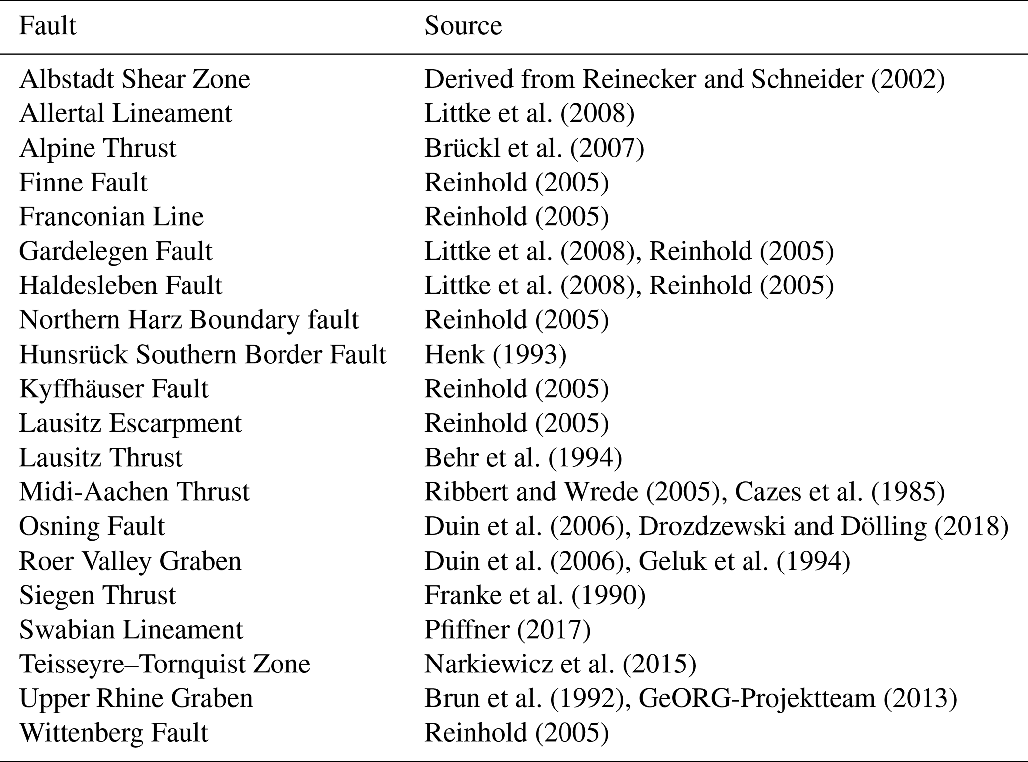
Semi-realistic fault set. For 23 faults, a more complex geometry on the basis of seismic and geological cross sections is used. The depth of the faults is not constant as in the Vertical and Andersonian fault sets but is chosen in accordance with the depths given in the sections used. The vertical cross sections used for the generation of the Semi-realistic fault set are compiled in Table 1. The quantity of available cross sections per fault varied considerably. For many faults, only one cross section was available leading to a uniform geometry over the entire length of the fault.
Table 1Sources with suitable geological and seismic cross sections for the generation of semi-realistic fault geometries and the specific faults they were used for.
2.4 Three-dimensional slip tendency analysis
To estimate the fault reactivation potential we use definitions and terms of Morris et al. (1996). Assuming that cohesion can be neglected, they defined the parameter slip tendency as the ratio between τ and σn. We use this definition as a first slip tendency type:
We further use three additional slip tendency parameters for our analysis. TSeff considers σneff, which takes the influence of pore pressure on σn (Jaeger et al., 2011) into account.
A normalization to μ has been used for example by Peters (2007) and is additionally calculated as TSnorm and TSnormeff. We choose μ as 0.57, which is in the middle of the range reported by Jaeger et al. (2011). For TSnorm and TSnormeff slip is likely to occur if they approach values around 1 or larger.
The pore pressure Pp for the calculation of σneff is computed from the depth z [m] (which is the true vertical depth below the topographic surface of the German stress model), gravity g [9.81 m s−2] and the fluid density ρ [1000 kg m−2]:
To estimate the slip tendencies, the fault geometries are discretized as surfaces with triangles with a side length of 800 m. Then the 3D stress tensor components from the geomechanical–numerical model of Ahlers et al. (2021b) are mapped onto the corner nodes of the triangles using Tecplot 360 EX v2019 and the Add-on Geostress (Heidbach et al., 2020). The mean stress tensor of the three nodes is multiplied with the normal vector of each triangle to estimate τ and σn. With the hydrostatic pore pressure, the four slip tendency parameters are calculated.
3.1 Vertical fault set
The results for the Vertical fault set are shown for all four slip tendency parameters in Fig. 2. As the faults are vertical, the top view only shows the values along the fault top. TS of the Vertical fault set ranges mainly between 0 and 0.5 (histograms are shown in Fig. S2 in the Supplement). Higher TS values are reached for the uppermost parts of some faults as can be seen in Fig. 2a. With increasing depth TS decreases rapidly to nearly 0 for all faults. Faults striking NNE–SSW and NW–SE show elevated TS values in the uppermost parts of the faults when compared to faults of other strike directions.
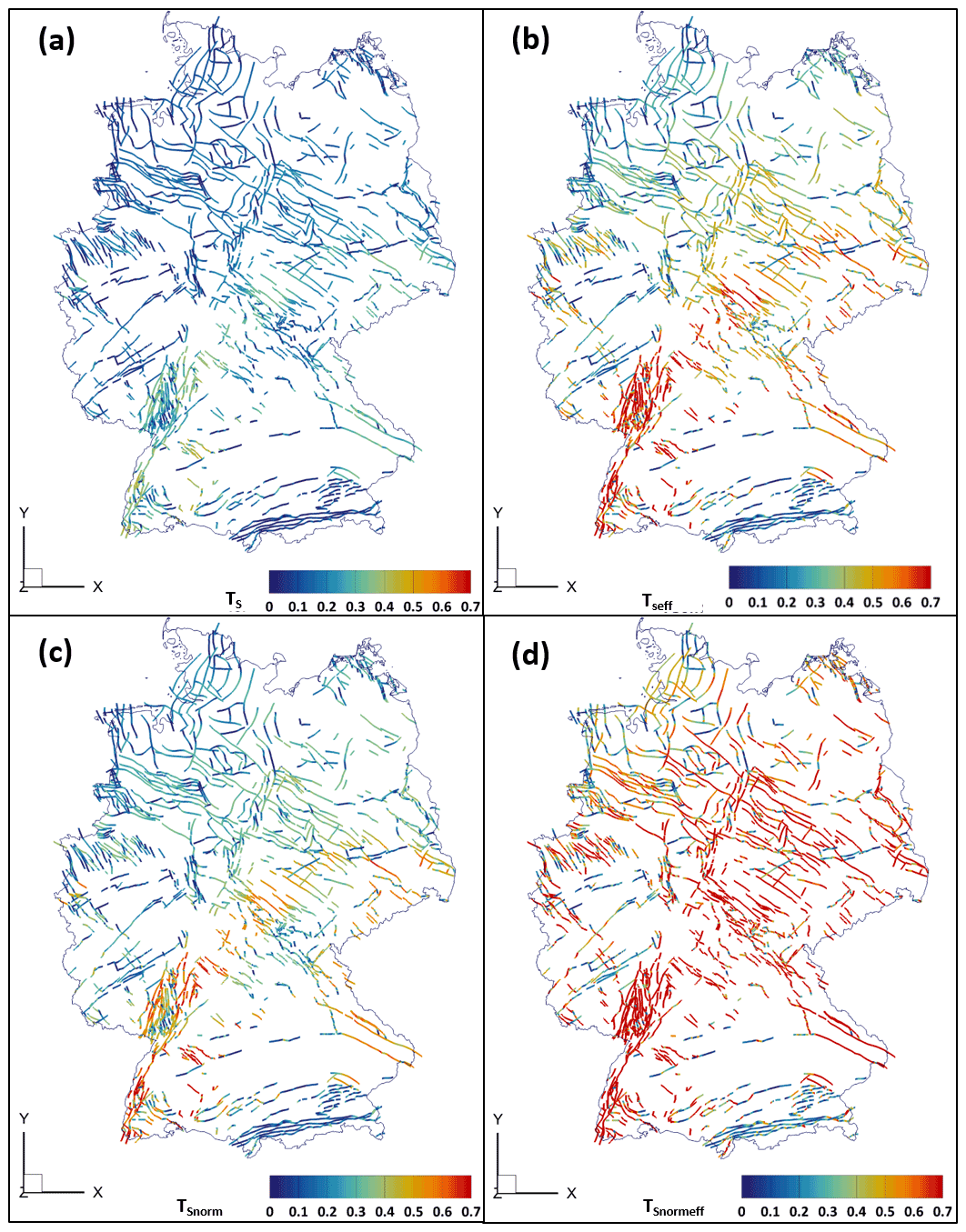
Figure 2Top view of the slip tendency of the Vertical fault set calculated for four cases. Due to the vertical nature of the faults only the uppermost parts of the faults are visible. (a) TS; (b) TSeff (with effective normal stresses); (c) TSnorm (normalized to a coefficient of friction of 0.57); (d) TSnormeff (with effective normal stresses and normalized to a coefficient of friction of 0.57). ©EuroGeographics for the administrative boundaries.
TSeff is higher than TS and ranges mainly between 0 and 0.7. TSeff is highest in the uppermost fault parts and decreases rapidly with increasing depth as well. NW–SE- and especially NNE–SSW-striking faults show higher TSeff than faults of other strike directions. TSnorm values mainly range between 0 and 0.7, and TSnormeff ranges mostly between 0 and 1. The same trends for depth and fault strike apply as for TS and TSeff. TSnorm and TSnormeff are however higher in the uppermost parts of the faults than TSeff.
3.2 Andersonian fault set
The resulting slip tendencies of the Andersonian fault set are shown for all four slip tendency types in Fig. 3 (additional histograms are given in Fig. S3). TS ranges mainly between 0 and 0.2. Only the uppermost parts of some NNW–SSE- and NE–SW-striking faults such as the URG, the Albstadt Shear Zone and the Landshut–Neuötting Fault show slightly higher values.
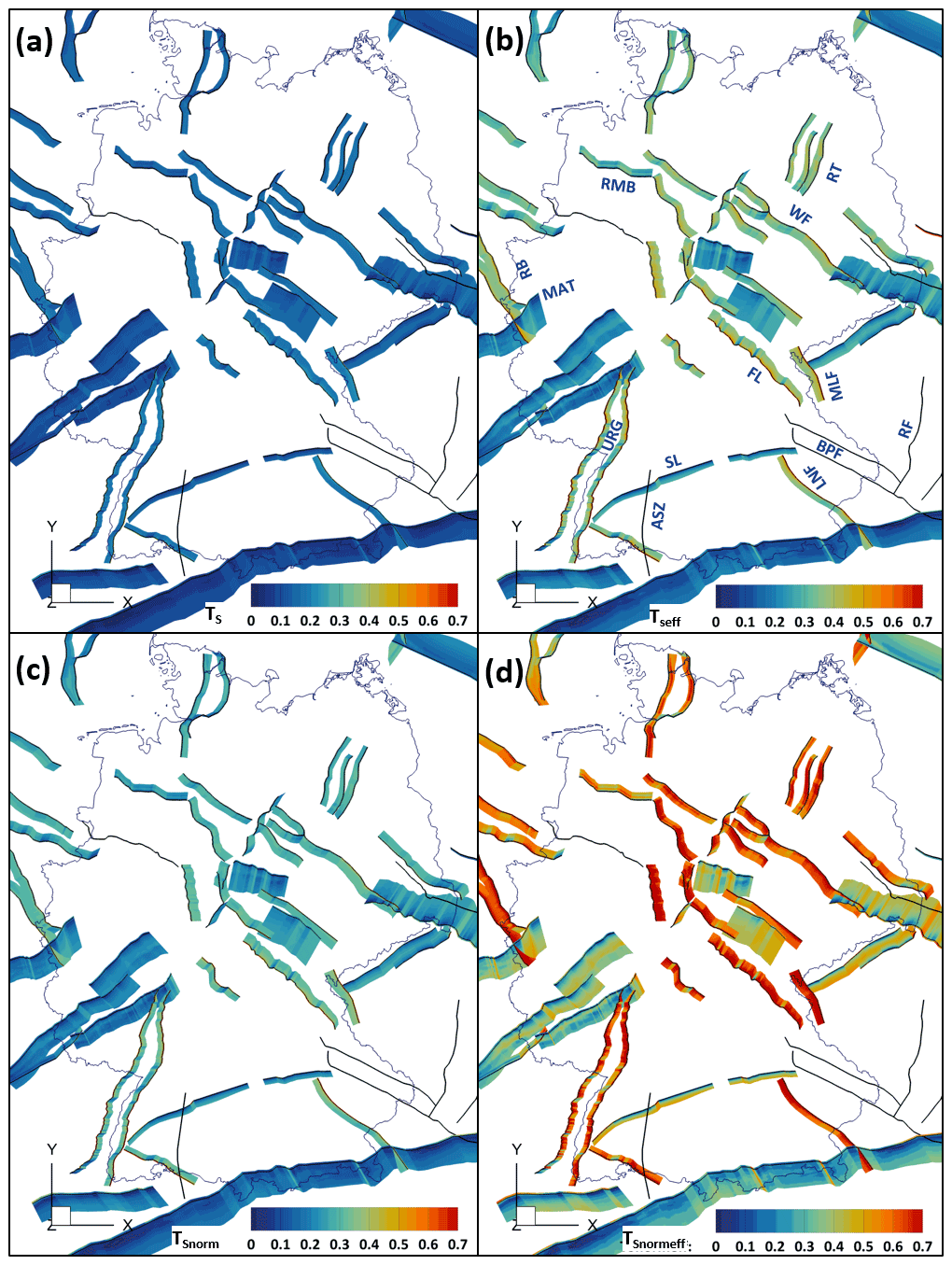
Figure 3Top view of the slip tendency of the Andersonian fault set calculated for four slip tendency types. (a) TS; (b) TSeff (with effective normal stresses); (c) TSnorm (normalized to a coefficient of friction of 0.57); (d) TSnormeff (with effective normal stresses and normalized to a coefficient of friction of 0.57). ASZ: Albstadt Shear Zone; BPF: Bavarian Pfahl Fault; FL: Franconian Line; LNF: Landshut–Neuötting Fault; MAT: Midi-Aachen Thrust; MLF: Mariánské Lázne Fault; URG: Upper Rhine Graben; RB: Roer Basin; RT: Rheinsberg Trough; RF: Rodl Fault; RMB: Rheder Moor–Blenhorst Fault; SL: Swabian Lineament; WF: Wittenberg Fault. ©EuroGeographics for the administrative boundaries.
TSeff mostly ranges between 0 and 0.4. Only 5 % of the values are higher than 0.4. TSeff is generally elevated for faults and fault segments striking in a NNE–SSW and NW–SE direction such as the URG, the Franconian Line, the Albstadt Shear Zone, the Wittenberg Fault, the Rheinsberg Trough, the Landshut–Neuötting Fault and the Roer Valley Graben. The influence of fault strike direction is especially prominent for faults with segments of varying orientation. The NW–SE-striking parts of the Rheder Moor–Blenhorst Fault show elevated TSeff values when compared to the more WNW–ESE-striking segments of the fault. For strike-slip faults, TSeff strongly decreases within the uppermost fault parts and keeps decreasing with increasing depth as shown for parts of the Albstadt Shear Zone in Fig. 4a. TSeff slightly increases with depth after the initial strong decrease for some normal and thrust faults. This is shown for the Midi-Aachen Thrust in Fig. 4b. TSnorm ranges mainly between 0 and 0.3 and shows an overall similar behavior to TSeff. While the high TSnormeff values reach up to 1.0, areas with low TSnormeff show values in the same range as for the other three slip tendency parameters. The spatial distribution of areas of low and high TSnormeff values is similar to TSnorm and TSeff.

Figure 4Vertical section of TSeff along faults. (a) TSeff of a northern part of the Albstadt Shear Zone decreases over the entire depth; (b) TSeff of an eastern part of the Midi-Aachen Thrust slightly increases again (after an initial strong decrease) as indicated by the shift from blue to greenish colors at greater depths. Color bar applies to both (a) and (b).
3.3 Semi-realistic fault set
Figure 5 shows the results of the slip tendency calculations for the Semi-realistic fault set; additional histograms are shown in Fig. S4. TS ranges mainly between 0 and 0.2. For the Semi-realistic fault set, the NNE–SSW- and NW–SE-striking faults show elevated TS compared to faults of other orientations. The highest TS can be observed at the uppermost steeply dipping sections of the URG, the Franconian Line, the Albstadt Shear Zone, the Wittenberg Fault and the Roer Valley Graben. For most faults, TS decreases with increasing depth. However, most faults are significantly less deep than in the Andersonian fault set.
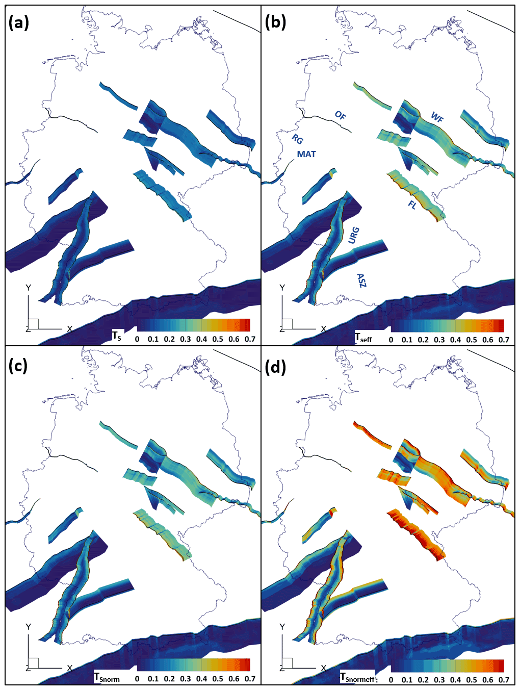
Figure 5The semi-realistic fault geometries are color-coded by their slip tendency for four cases. (a) TS; (b) TSeff (with effective normal stresses); (c) TSnorm (normalized to a coefficient of friction of 0.57); (d) TSnormeff (with effective normal stresses and normalized to a coefficient of friction of 0.57). ASZ: Albstadt Shear Zone; FL: Franconian Line; MAT: Midi-Aachen Thrust; OF: Osning Fault; URG: Upper Rhine Graben; RG: Roer Valley Graben; WF: Wittenberg Fault. ©EuroGeographics for the administrative boundaries.
TSeff ranges mainly between 0 and 0.4 with 5 % of values 0.5 or higher. Faults striking in a NNW–SSE and NE–SW direction such as the URG, the Franconian Line, the Albstadt Shear Zone, the Wittenberg Fault and the Roer Valley Graben show elevated TSeff as compared to faults of other strike directions. This influence is especially noticeable for the Franconian Line where the WNW–ESE-striking segments of the fault show lower TSeff than the NNW–SSE-striking ones. For sections of the uppermost parts of the URG and the Roer Valley Graben TSeff exceeds values of 1. The decrease in TSeff with increasing depth is especially prominent for faults that have been implemented with a listric geometry (such as the URG or the Hunsrück Southern Border Fault). While the listric URG geometry shows some of the highest TSeff values for the Semi-realistic fault set in its uppermost parts, TSeff decreases drastically with depth. The same decrease can be observed for the listric Hunsrück Southern Border Fault. In contrast, TSeff increases drastically in the lowermost part of the Swabian Lineament after a steady decrease in TSeff with increasing depth for the most part of the fault.
TSnorm mainly ranges between 0 and 0.4 The TSnorm distribution is almost identical to the one of TSeff. TSnormeff mainly ranges between 0 and 0.8. The high TSnormeff values mainly occur on the NW–SE- and NNE–SSE-striking faults, while the areas with low TSnormeff show values similar to the other slip tendency types in the respective areas.
4.1 Influence of fault strike on slip tendency
To investigate the influence of the spatial orientation of the faults on the slip tendency, we prepared scatterplots of TSeff as a function of fault strike for all faults of each of the three fault sets (Fig. 6). The normal faults, thrust faults and strike-slip faults of the Andersonian set are displayed in separate subfigures (Fig. 6b, c and d, respectively).
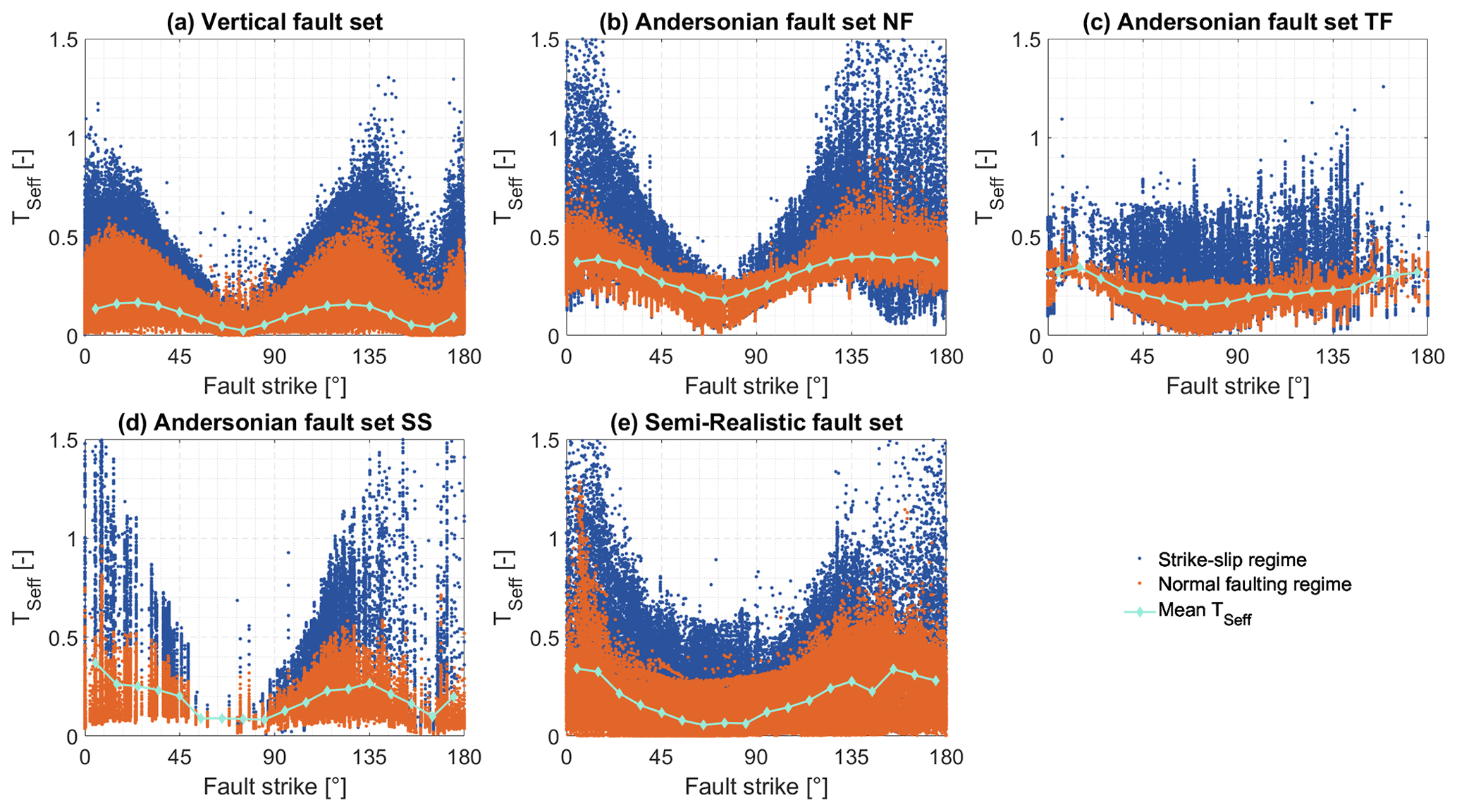
Figure 6Scatterplots showing TSeff and the fault strike of each node of the fault mesh. Additionally, the stress regime the data points are subjects to is indicated by its color (blue for strike-slip regime, orange for normal faulting regime). The mean TSeff in 10∘ fault strike steps is plotted as a mint-colored line. (a) Vertical fault set; (b) normal faults of the Andersonian fault set; (c) thrust faults of the Andersonian fault set; (d) strike-slip faults of the Andersonian fault set; (e) Semi-realistic fault set.
Overall, the minimum TSeff values occur consistently at strikes of 75∘ for all fault types, i.e., the reactivation potential is generally the lowest for ENE–WSW-striking faults, as could be expected in the context of the stress orientation shown in Fig. 1c and d. Vertical faults also show a low reactivation potential on NNW–SSE-striking segments (corresponding to strikes of 165∘). The maximum TSeff occurs for strikes of 5–25∘ for all fault types, i.e., the reactivation potential is generally highest for N–S to NNE–SSW-striking faults; these faults strike at an angle of 25∘ to SHazi with an orientation between 160 and 175∘. The vertical faults also have a high reactivation potential for NW–SE strikes, the Andersonian normal faults for NNW–SSE-striking segments. Due to the uniform dip of the Vertical fault set, dip is not a variable of influence for this fault set and only the location in the stress field and the strike of the fault lead to differences in slip tendency.
4.2 Influence of depth and shear stress on slip tendency
For all three fault sets, a strong decrease in the slip tendencies can be observed from the surface to a depth of 5–10 km as shown in Figs. 7 and 8 for the Vertical and Andersonian fault sets, respectively. At greater depths, the slip tendency gradient is low. This is the case for all four slip tendency types. For the Vertical fault set (Fig. 7), slip tendency decreases steadily for all four slip tendency types with the exception of a dent between 32 and 38 km. However, since only very few fault segments reach this depth, the influence of fault strike strongly superimposes the depth dependency for these depths. For the Andersonian fault set (Fig. 8), the same trends apply in general as for the Vertical fault set. However, for the thrust and normal faults the initial strong decrease in slip tendency occurs within the uppermost 3–4 km. At this depth, the stress regime switches from a strike-slip regime to a normal faulting regime in most parts of the model. The slip tendencies of the strike-slip faults are generally higher than the ones of the thrust and normal faults in the upper 5–10 km but generally lower at greater depths. In contrast to the strike-slip faults, both normal and thrust faults show a slight increase in the mean slip tendency with increasing depth below 5 km depth. The mean slip tendency increase with depth is higher for the thrust faults than for the normal faults.
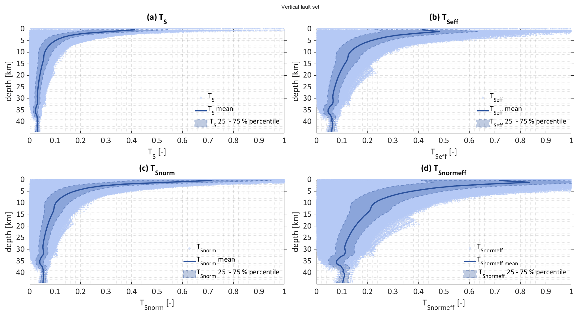
Figure 7All slip tendency data are plotted vs. depth for the Vertical fault set. The mean slip tendency is plotted as a solid line; the 25 %–75 % percentile is shown as a shaded area.
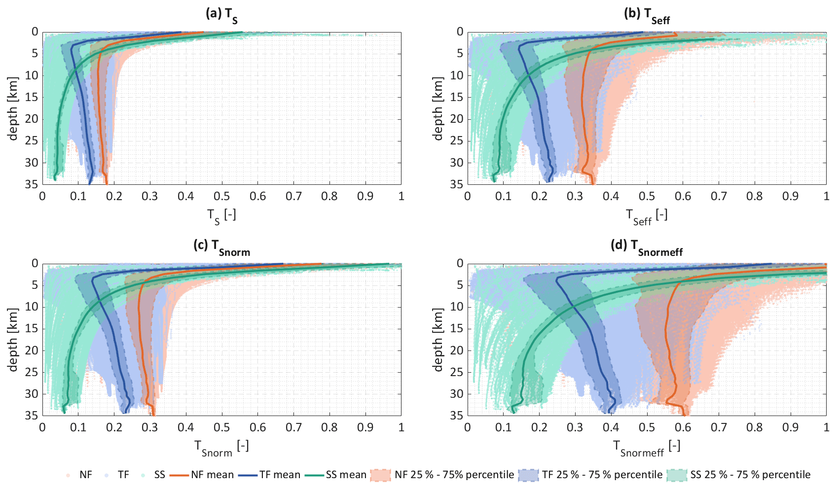
Figure 8All four slip tendency types at each data point of the Andersonian fault set are plotted vs. their depth. The mean slip tendency is plotted as a solid line; the 25 %–75 % percentile is shown as a shaded area. Due to the different behavior of normal, thrust and strike-slip faults, the three fault types are colored individually. Data corresponding to the normal faults are shown in orange, data corresponding to thrust faults are shown in blue, and data corresponding to strike-slip faults are shown in mint color.
For normal, thrust and strike-slip faults σn increases at a similar rate with increasing depth. On the other hand, τ on strike-slip faults and the faults of the Vertical fault set increases less strongly. Since slip tendency has been defined as , low τ leads to low slip tendencies for the strike-slip faults and the faults of the Vertical fault set. Figure 9 shows τ for the Vertical fault set. Additionally, σneff, τ and the resulting TSeff of the Landshut–Neuötting Fault are shown exemplarily. While σneff increases to over 250 MPa, τ only increases to around 20 MPa at a depth of 30 km (note that the range of the color bar of σneff is 10 times the range of the τ). This results in TSeff strongly decreasing with increasing depth for all faults regardless of their strike direction in the Vertical fault set.
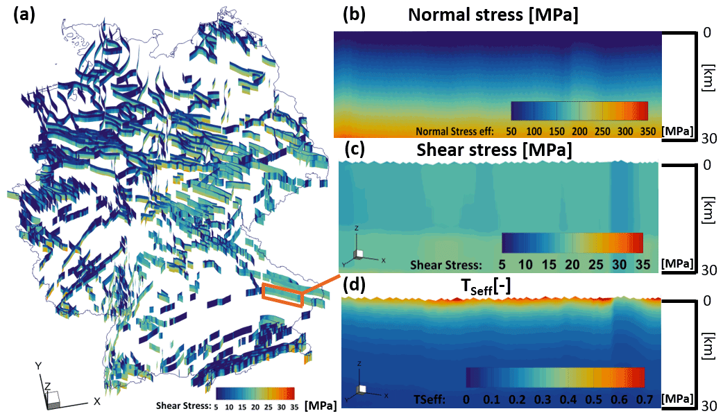
Figure 9(a) Shear stress τ in MPa of the Vertical fault set with the color map ranging from 5 to 35 MPa (oblique view). (b)–(d) Zoomed in view of the Landshut–Neuötting Fault normal to the strike reaching to a depth of around 30 km; (b) effective normal stress σneff with the color map ranging from 50 to 350 MPa; (c) shear stress τ with the color map ranging from 5 to 35 MPa; (d) TSeff of the Landshut–Neuötting Fault is shown with the color map ranging between 0 and 0.7. ©EuroGeographics for the administrative boundaries.
4.3 Influence of fault dip
In order to investigate the influence of the 3D fault geometry, we compare the slip tendency histograms of the Vertical (blue), Andersonian (orange) and Semi-realistic (mint) fault set (Fig. 10). For all four slip tendency types, the Vertical fault set shows a right-skewed bell shape, the Semi-realistic fault set displays as J shape, and the Andersonian fault set shows a bimodal distribution. The bimodal character of the Andersonian fault set is more distinct for TSeff and TSnormeff. The slip tendency values of the first peak are mainly concentrated on the thrust faults, whereas the slip tendency values of the second peak are mainly present on normal faults.
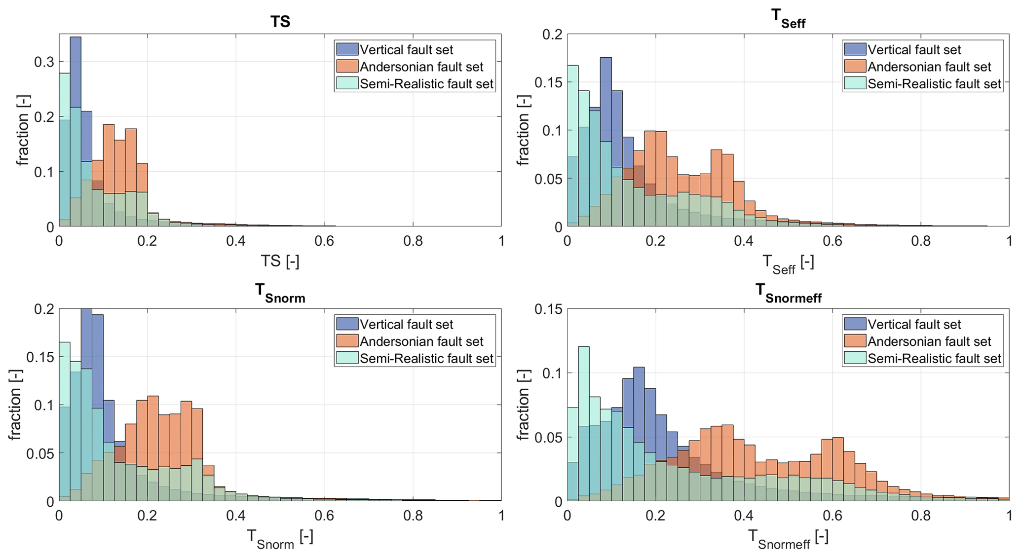
Figure 10Comparison of the slip tendency histograms of the Vertical (blue), Andersonian (orange) and Semi-realistic (mint) fault set for the four slip tendency types. Slip tendency values greater than 1 are not shown. The slip tendency values have been calculated on the nodes of the fault mesh; mesh resolution is 800 m for all three fault sets. Bin size is 0.025.
As the normal faulting regime is predominant in most parts of the Germany model (especially at depths greater than 4 km) in general σn is lower for normal faults than for thrust faults, which have been implemented with a dip of 60 and 30∘, respectively, in the Andersonian fault set, leading to the bimodal distribution of TS.
The more prominent bimodal distribution of TSeff and TSnormeff in the Andersonian fault set results from the influence of the calculation of the pore pressure as a function of depth. In combination with the normal faulting regime in most parts of the Germany model, this leads to a stronger relative reduction in σneff for normal faults than for thrust faults.
The listric geometry of the URG in the Semi-realistic fault set is based on DEKORP 9N (Brun et al., 1992). The URG shows high TSeff values in the uppermost parts for both the Andersonian and the Semi-realistic fault set. With increasing depth, the dip of the Semi-realistic URG faults decreases until it becomes sub-horizontal. This decrease in dip coincides with a significant TSeff decrease. In contrast, TSeff for the Andersonian fault geometries decreases at a significantly lower rate. This results from the fact that while σneff increases at a similar rate for both fault types, τ of the Semi-realistic URG increases at a much lower rate than it does for the Andersonian URG (also shown in Fig. S5). Results from the Hunsrück Southern Border Fault, another listric fault, (derived from DEKORP 9N and 1C, Henk, 1993) show a similar behavior.
The overall low slip tendency values of the Vertical fault set were to be expected due to the prevailing normal faulting regime in most parts of the model and the uniform 90∘ dip of the Vertical fault set. The low values do not properly reflect the actual fault reactivation potential of faults with different dips in reality. The reactivation potential for faults with other dips in reality is underestimated in areas with normal and thrust faulting regimes and overestimated in a strike-slip regime.
4.4 Influence of pore pressure
The use of a hydrostatic pore pressure is a major simplification since the pore pressure is not hydrostatic everywhere in Germany. Considerable overpressures have been shown for example in the Molasse Basin (Drews et al., 2018; Müller et al., 1988). Müller et al. (1988) describes pore pressure gradients of up to 24 MPa km−1 in the vicinity of the lineament of the Alpine Thrust. Figure 11 shows TSeff for the Alpine Thrust for pore pressure gradients of (a) 10 MPa km−1 (hydrostatic) (b) 16 MPa km−1 and (c) 22 MPa km−1. TSeff increases drastically with increasing pore pressure. For the gradient of 16 MPa km−1 TSeff reaches values of up to 0.7 for favorably oriented segments of the fault. For a pore pressure gradient of 22 MPa km−1 TSeff increases to over 0.7 for almost all parts of the fault and reaches values well in excess of 1 over large areas. Even though these pore pressure gradients are unlikely to occur over large areas of the fault, this highlights the crucial impact of the pore pressure on the fault reactivation potential.
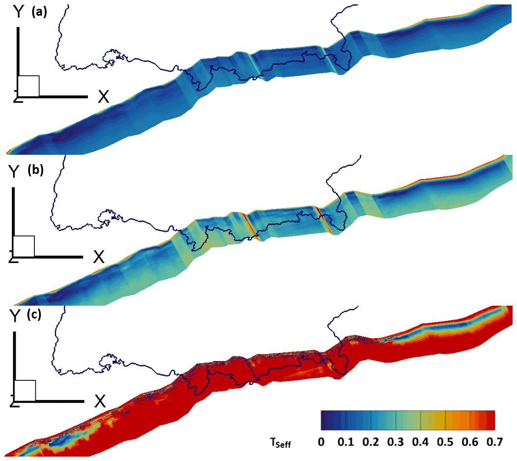
Figure 11TSeff of the Alpine Thrust for different pore pressures. (a) TSeff with hydrostatic pore pressure corresponding to a gradient of 10 MPa km−1; (b) TSeff for an overpressured pore pressure with a gradient of 16 MPa km−1; (c) TSeff for an overpressured pore pressure with a gradient of 22 MPa km−1. The color bar applies to all three cases. ©EuroGeographics for the administrative boundaries.
4.5 Comparison between slip tendency and seismicity
In order to evaluate our slip tendency results, we test them qualitatively against the distribution of tectonic earthquakes. The earthquakes are taken from the EMEC seismic event catalogue of Grünthal and Wahlström (2012) that covers the period between 1000 to 2006 CE in the investigation area and provides earthquakes with magnitudes Mw≥ 3.5. We added events to this compilation with Mw≥ 3.5 for the years 2007–2021 from the GEOFON data center at the GFZ German Research Centre (Quinteros et al., 2021). For the events with a given hypocentral depth, the majority occur at 8 km (refer to Fig. S6), and the largest moment magnitudes are observed at 8 to 10 km depth. Therefore, we use the slip tendency values at a cross section at 8 km depth for the comparison with seismic events.
Figure 12a shows the location of the seismic events with Mw≥ 3.5 color-coded by their moment magnitude alongside a horizontal cross section through the Vertical fault set at a depth of 8 km. The faults are color-coded by their TSeff values. The overall TSeff at this depth is very low with values of only up to 0.3 as the 90∘ dip is unfavorable for reactivation in the normal faulting regime at this depth. However, the NNE–SSW-striking faults of the seismically active Upper Rhine area show slightly higher TSeff values than other areas with low seismicity. While several seismic events in east Germany are localized close to faults with elevated TSeff, there are several faults with similar or higher values where no seismicity is documented. The seismicity in the Roer Valley Graben area and its SE-trending elongation is localized along faults where only some segments show slightly elevated TSeff values or where no faults at all have been mapped. While the Vertical fault set is based on a very comprehensive fault selection it is apparent from the distribution of seismic events that some relevant structures are likely still missing.
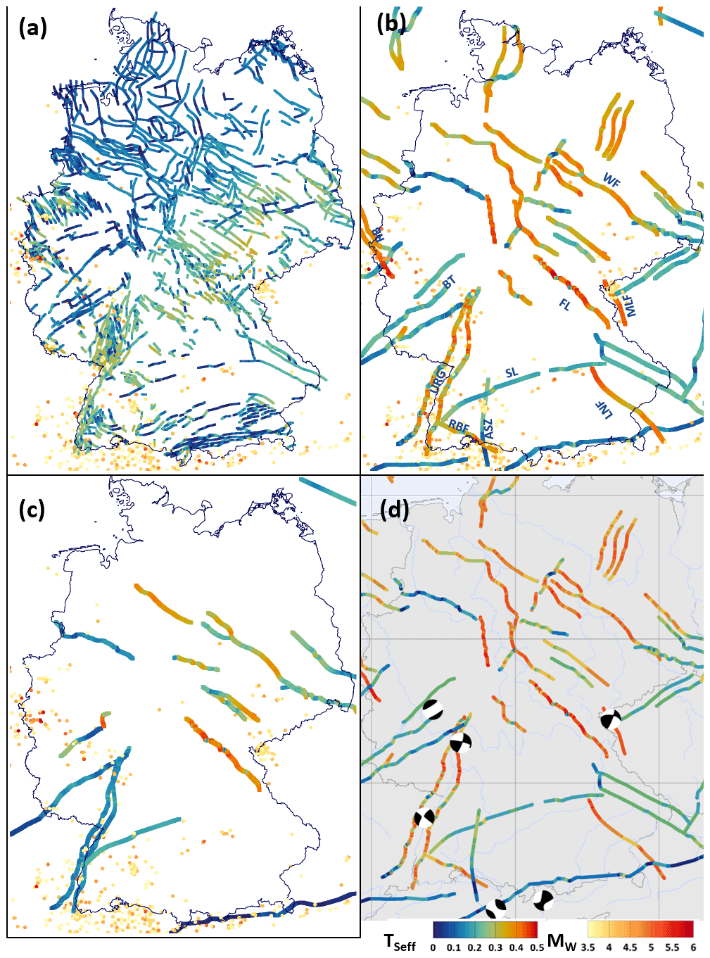
Figure 12Seismic events with Mw>3.5 color-coded by their moment magnitude (yellow to red) displayed on horizontal cross sections through the fault sets color-coded by TSeff (hydrostatic pore pressure) at 8 km depth. (a) Vertical fault set; (b) Andersonian fault set; (c) Semi-realistic fault set. The color bars of Tseff and Mw apply to (a)–(d); (d) Andersonian fault set with fault plane solutions from the GFZ GEOFON catalogue (Quinteros et al., 2021) visualized using the focalmech script (Conder, 2022). ASZ: Albstadt Shear Zone; BT: Boppard Thrust; LNF: Landshut–Neuötting Fault; MLF: Mariánské Lázne Fault; RBF: Randen–Bonndorf Fault; RB: Roer Basin; SL: Swabian Lineament; URG: Upper Rhine Graben. ©EuroGeographics for the administrative boundaries.
This is not surprising when considering the results of fault detection using photo-lineations derived from high-resolution data of satellite missions such as the European Remote Sensing Satellite (ERS) 1/2. For example, Franzke and Wetzel (2001) present in their work for southern Germany that there are numerous additional fault networks on a smaller scale that could potentially serve as faults for the catalogued seismicity with small magnitudes. However, if we only used large events with Mw>6 instead that, according to empirical relations, have a rupture length of >10 km (Wells and Coppersmith, 1994), these would fit our resolution better, but in a low-strain area these magnitudes do not occur very often and even the largest recorded event in Germany from the year 1911 with Mw 5.8 in the Albstadt Shear Zone would not be usable; only the historical events where the epicenter estimation based on intensity reports is highly uncertain could be used.
A cross section through the Andersonian fault set at a depth of 8 km is shown in Fig. 12b; the same color codes as for Fig. 12a apply. The occurrence of seismic events is in good accordance with the elevated TSeff of the URG, the Roer Valley Graben, the Mariánské Lázne Fault and the Randen–Bonndorf Fault. However, especially in east Germany and in the SE-trending elongation of the Roer Valley Graben there are areas without faults despite numerous seismic events. Furthermore, TSeff is rather low along the Albstadt Shear Zone, one of the seismically most active areas in Germany due to the implementation as a 90∘-dipping strike-slip fault. In contrast, there are also areas with TSeff in the same range as the URG with no or only very little seismicity, especially in northern Germany. Here, TSeff is either overestimated in comparison to seismically active areas or stress relief is achieved by other processes.
Since only a subset of the Andersonian fault set could be implemented in the Semi-realistic fault set, there are many areas where earthquakes occur but no fault geometry is considered (Fig. 12c). While the shallow sections of the URG and the Albstadt Shear Zone show TSeff of 0.6 and higher, TSeff is relatively low at a depth of 8 km. In general, TSeff is lower at the 8 km depth cross section for the Semi-realistic fault set than for the Andersonian fault set.
While some of the seismogenic areas show elevated TSeff values, the absolute values are rather low, especially at 8 km depth and deeper, where most of the considered seismic events take place. If μ is low enough, seismicity can still occur even with TSeff in the range below 0.4. The range of μ of faults can vary greatly and even reach values below 0.4 for faults with fault gouge (Numelin et al., 2007; Haines et al., 2014) as a compilation by Ferrill et al. (2017) shows. For higher μ, as they have been shown for different locations (Zoback and Healy, 1992, 1985; Brudy et al., 1997) and collected by Peters (2007), TSeff would need to reach higher values in order to explain seismic events. This could be achieved through higher τ or lower σn. In order to achieve these, either significant changes regarding the stress tensor from the geomechanical model of Germany or changes in the fault geometry would be required. The changes to the stress tensor required would not be warranted by the calibration data used for the model of Germany. In order to elevate TSeff of the Franconian Line to values of 0.7 and higher, an additional 30 MPa of τ would be required at 8 km depth. The required stress changes however would not fit the data from the kontinentale Tiefbohrung (German Continental Deep Drilling Program) (KTB) nearby that has been used for the model calibration. On the other hand, the fault geometries are subject to major uncertainties due to the sparse data available on the geometries at greater depths. As shown above, both fault strike and fault dip drastically impact the resulting slip tendency, and the uncertainties regarding the 3D fault geometries could therefore at least partly explain the overall low values.
A comparison of the faults of the Andersonian fault set with three fault plane solutions (Quinteros et al., 2021) (Fig. 12d) shows that one of the nodal planes' strike is (sub-) parallel to the URG, even though the corresponding dips are steeper at around 75∘ than they were assumed for the URG in the Andersonian fault set. For the Alpine Thrust, one fault plane solution in the fault's proximity shows a parallel strike of 78∘ but a much steeper dip of 71∘ than the 30∘ dip that had been assumed for the Alpine Thrust, with another fault plane solution indicating reactivation along a fault that is not present in the fault set. A fault plane solution close to the NNW–SSE-striking Mariánské Lázne Fault indicates seismicity linked to a NNE–SSW-striking fault. Reactivation along a fault striking in a NNW–SSE direction rather than NE–SW direction is indicated by a fault plane solution in the area of the NE–SW-striking Boppard Thrust. Such faults are present in the Vertical fault set, even though their slip tendencies are rather low due to the 90∘ dip in the normal faulting regime. Even though the Andersonian fault set roughly replicates the general fault pattern documented for Germany, a more diverse fault set in terms of strike, location and dip is required for a more comprehensive comparison with the seismic events.
4.6 Data limitations
The relevant data for this slip tendency analysis are the stress tensor, pore pressure, frictional fault properties and fault geometry. The model by Ahlers et al. (2021b), which provides the 3D absolute stress tensor for our study, has a coarse resolution and only implements a single sediment layer as well as only four upper crustal units. Tectonic faults are not implemented and thus local stress variations due to their presence are not considered in the model. Ahlers et al. (2021a) describe a good fit to the stress magnitude data that are used for the model calibration. However, these are located in the uppermost kilometers of the model where we predict the overall highest slip tendencies. At greater depths, where our slip tendency results are visibly lower, no calibration data were available for the geomechanical model.
Wide regions and depth intervals of the numerical model indicate a prevailing normal faulting stress regime. However, focal mechanisms of seismic events (Heidbach et al., 2016) indicate a possible strike-slip regime also at greater depths. In such a regime, an overestimation of the minimum horizontal stress Shmin reduces the slip tendencies. Similarly, the underestimation of the maximum stress (either the vertical stress Sv in normal faulting stress regime or the maximum horizontal stress SHmax in a strike-slip stress regime) might explain the low slip tendencies.
A second major source of uncertainty results from the limited data available regarding the 3D fault geometries of the selected faults with sufficient depth extension (mostly >5 km). Only few seismic sections and geological cross sections could be used for the 3D fault geometry generation. Due to the sparse data available for most faults the 3D geometry has been deduced from only one section. The resulting geometries are therefore unlikely to properly represent the real 3D fault geometries (dip, strike, depth extent) over the entire fault lengths. As shown above, strike and dip have major influences on the resulting slip tendency.
Pore pressure data are too sparse to justify the discrimination of areas of distinct pore pressure gradients and thus only a hydrostatic pore pressure could be assumed for the estimation of TSeff and TSnormeff with the abovementioned effects. Since data on the frictional fault properties were not available, we assumed the faults to be cohesionless. If the considered faults have cohesion greater than 0, the resulting slip tendencies would be further reduced.
4.7 Comparison with earlier studies
Peters (2007) analyzed the slip tendency of the URG with the help of a numerical model. Using a dip of 60∘ for faults with a known dip direction and assuming hydrostatic pore pressure calculated slip tendencies reached values of up to 0.8 at a depth of 2.5 km and with a normalization to a coefficient of friction of 0.4. Even though the slip tendency in this study has been normalized to a higher coefficient of friction of 0.6 the overall slip tendency values in this study are around 0.2 higher than the results in Peters (2007). However, the URG boundary faults show elevated values for similar segments to the ones in the study by Peters (2007). The study of Worum et al. (2004) calculates TSeff values between 0.2 and 0.4 for the Roer Valley Graben using an analytical model for faults reaching depths of around 2–3 km for comparable ratios and the strike-slip regime that is present in the Germany model at the before mentioned depths. TSeff of the Roer Valley Graben boundary faults in this study ranges between 0.6 for the southernmost parts of the faults and 0.2 in the northern parts, which is in contrast to the trends displayed in Worum et al. (2004), where the southern parts of the faults show the lowest TSeff values. However, the high TSeff values appear on short segments with ideal orientation for reactivation under the given strike-slip regime with SHazi around 155∘. Slightly less well-oriented segments show values that are in better agreement with the results by Worum et al. (2004).
The slip tendency analysis on basis of the 3D absolute stress tensor from the geomechanical–numerical model of Germany (Ahlers et al., 2021b) allowed the identification of regions with a higher reactivation potential and regions where faults are more stable. Elevated slip tendencies have been found especially for NNE–SSW- and NW–SE-striking faults such as the URG, the Franconian Line, the Albstadt Shear Zone, the Wittenberg Fault, the Rheinsberg Trough, the Landshut–Neuötting Fault and the Roer Valley Graben. However, a comparison with focal mechanisms points towards reactivation of a more diverse set of faults, which should be subject to further studies.
The major influence of fault geometry on the calculated slip tendency has been shown by the comparison of three fault sets. High-quality information on fault geometry can be provided for example by interpreted seismic sections for large-scale faults. To improve this kind of analysis, faults should be characterized by multiple seismic cross sections. The analysis has also shown the crucial influence of the pore pressure on slip tendencies for the fault sets considered. However, no spatially comprehensive pore pressure data for the entire area of Germany are available. The same applies for the frictional properties of faults, which are only poorly restrained. Lastly, further and more information on the stress state in Germany is crucial for a more reliable slip tendency analysis.
The fault geometries are available under the DOI https://doi.org/10.5445/IR/1000143465 (Röckel et al., 2022).
The supplement related to this article is available online at: https://doi.org/10.5194/se-13-1087-2022-supplement.
Conceptualization of the project was done by AH, TH, KR, OH, FS and BM. Research and collection of fault information was done by SA and LR. Generation of 3D fault geometries and slip tendency analysis were done by LR. Evaluation and interpretation of the slip tendency results were done by LR with the support of BM, OH, KR, TH, SA and AH. LR wrote this paper with the help of all coauthors. All authors read and approved the final paper.
The contact author has declared that neither they nor their co-authors have any competing interests.
Publisher’s note: Copernicus Publications remains neutral with regard to jurisdictional claims in published maps and institutional affiliations.
This study is part of the SpannEnD Project (http://www.SpannEnD-Projekt.de, last access: 25 February 2022), which is supported by Federal Ministry for Economic Affairs and Energy (BMWI) and managed by Projektträger Karlsruhe (PTKA) (project code: 02E11637A). We acknowledge support by the KIT Publication Fund of the Karlsruhe Institute of Technology.
This research has been supported by the Bundesministerium für Wirtschaft und Energie (grant no. 02E11637A).
The article processing charges for this open-access publication were covered by the Karlsruhe Institute of Technology (KIT).
This paper was edited by David Healy and reviewed by David Ferrill and Stephen Hicks.
Agemar, T., Alten, J.-A., Gorling, L., Gramenz, J., Kuder, J., Suchi, E., Moeck, I., Weber, J., V. Hartmann, H., Stober, I., Hese, F., and Thomsen, C.: Verbundsvorhaben “StörTief”: Die Rolle von tiefreichenden Störungszonen bei der geothermischen Energienutzung, Endbericht, 2016.
Ahlers, S., Henk, A., Hergert, T., Reiter, K., Müller, B., Röckel, L., Heidbach, O., Morawietz, S., Scheck-Wenderoth, M., and Anikiev, D.: 3D crustal stress state of Germany according to a data-calibrated geomechanical model, Solid Earth, 12, 1777–1799, https://doi.org/10.5194/se-12-1777-2021, 2021a.
Ahlers, S., Henk, A., Hergert, T., Reiter, K., Müller, B., Röckel, L., Heidbach, O., Morawietz, S., Scheck-Wenderoth, M., and Anikiev, D.: The Crustal stress state of Germany – Results of a 3D geomechnical model, TUdatalib [data set], https://doi.org/10.48328/tudatalib-437, 2021b.
Aleksandrowski, P., Kryza, R., Mazur, S., and Zaba, J.: Kinematic data on major Variscan strike-slip faults and shear zones in the Polish Sudetes, northeast Bohemian Massif, Geol. Mag., 134, 727–739, https://doi.org/10.1017/S0016756897007590, 1997.
Badura, J., Zuchiewicz, W., Stepancikova, P., Przybylski, B., Kontny, B., and Cacon, S.: The Sudetic Marginal Fault: a young morphophotectonic feature at the ne margin of the Bohemian Massif, Central Europe, Acta Geodyn. Geomater., 148, 7–29, 2007.
Behr, H. J., Duerbaum, H. J., Bankwitz, P., Bankwitz, E., Benek, R., Berger, H. J., Brause, H., Conrad, W., Foerste, K., Frischbutter, A., Gebrande, H., Giese, P., Goethe, W., Guertler, J., Haenig, D., Haupt, M., Heinrichs, T., Horst, W., Hurtig, E., and Kaempf, H.: Crustal structure of the Saxothuringian Zone; results of the deep seismic profile MVE-90(East), Z. Geol. Wissenschaft., 22, 647–770, 1994.
Bönnemann, C., Schmidt, B., Ritter, J., Gestermann, N., Plenefisch, T., and Wegler, U.: Das seismische Ereignis bei Landau vom 15. August 2009 – Abschlussbericht der Expertengruppe Seismisches Risiko bei hydrothermaler Geothermie, Bundesanstalt für Geowissenschaften und Rohstoffe, Hannover, 2010.
Brückl, E., Bleibinhaus, F., Gosar, A., Grad, M., Guterch, A., Hrubcová, P., Keller, G. R., Majdański, M., Šumanovac, F., Tiira, T., Yliniemi, J., Hegedűs, E., and Thybo, H.: Crustal structure due to collisional and escape tectonics in the Eastern Alps region based on profiles Alp01 and Alp02 from the ALP 2002 seismic experiment, J. Geophys. Res.-Sol. Ea., 112, 1109, https://doi.org/10.1029/2006JB004687, 2007.
Brudy, M., Zoback, M. D., Fuchs, K., Rummel, F., and Baumgärtner, J.: Estimation of the complete stress tensor to 8 km depth in the KTB scientific drill holes: Implications for crustal strength, J. Geophys. Res., 102, 18453–18475, https://doi.org/10.1029/96JB02942, 1997.
Brun, J. P., Gutscher, M.-A., and dekorp-ecors teams: Deep crustal structure of the Rhine Graben from dekorp-ecors seismic reflection data: A summary, Tectonophysics, 208, 139–147, https://doi.org/10.1016/0040-1951(92)90340-C, 1992.
Buchmann, T. J. and Connolly, P. T.: Contemporary kinematics of the Upper Rhine Graben: A 3D finite element approach, Global Planet. Change, 58, 287–309, https://doi.org/10.1016/j.gloplacha.2007.02.012, 2007.
BGR, LAGB, LBEG, LBGR, LLUR, and LUNG: 3D-Modell des geologischen Untergrundes des Norddeutschen Beckens (Projekt TUNB): Erstveröffentlichung 2021, Version 2022, https://gst.bgr.de (last access: 15 June 2022), 2021, Allgemeine Geschäftsbedingungen, siehe https://www.bgr.bund.de/AGB (last access: 27 June 2022), General terms and conditions, see https://www.bgr.bund.de/AGB_en (last access: 27 June 2022), 2021.
Cazes, M., Torreilles, G., Bois, C., Damotte, B., Galdeano, A., Hirn, A., Mascle, A., Matte, P., van Ngoc, P., and Raoult, J. F.: Structure de la croute hercynienne du Nord de la France; premiers resultats du profil ECORS, B. Soc. Geol. Fr., 8, 925–941, https://doi.org/10.2113/gssgfbull.I.6.925, 1985.
Conder, J.: focalmech James Conder, focalmech (fm, centerX, centerY, diam, varargin), MATLAB Central File Exchange [code], https://de.mathworks.com/matlabcentral/fileexchange/61227-focalmech-fm-centerx-centery-diam-varargin, last access: 27 June 2022.
Cornet, F. H. and Röckel, T.: Vertical stress profiles and the significance of “stress decoupling”, Tectonophysics, 581, 193–205, https://doi.org/10.1016/j.tecto.2012.01.020, 2012.
Drews, M. C., Seithel, R., Savvatis, A., Kohl, T., and Stollhofen, H.: A normal-faulting stress regime in the Bavarian Foreland Molasse Basin? New evidence from detailed analysis of leak-off and formation integrity tests in the greater Munich area, SE-Germany, Tectonophysics, 755, 1–9, https://doi.org/10.1016/j.tecto.2019.02.011, 2019.
Drews, M., Bauer, W., and Stollhofen, H.: Porenüberdruck im Bayrischen Molassebecken, Overpressure in the Bavarian Molasse Basin, Erdöl-Erdgas-Kohle, 12, 308–310, https://doi.org/10.19225/180703, 2018.
Drozdzewski, G. and Dölling, M.: Elemente der Osning-Störungszone (NW-Deutschland): Leitstrukturen einer Blattverschiebungszone, scriptum online, 2018.
Duin, E. J. T., Doornenbal, J. C., Rijkers, R. H. B., Verbeek, J. W., and Wong, T. E.: Subsurface structure of the Netherlands – results of recent onshore and offshore mapping, Neth. J. Geosci., 85, 245–276, https://doi.org/10.1017/S0016774600023064, 2006.
Evans, K. F., Zappone, A., Kraft, T., Deichmann, N., and Moia, F.: A survey of the induced seismic responses to fluid injection in geothermal and CO2 reservoirs in Europe, Geothermics, 41, 30–54, https://doi.org/10.1016/j.geothermics.2011.08.002, 2012.
Ferrill, D. A., Morris, A. P., McGinnis, R. N., Smart, K. J., Wigginton, S. S., and Hill, N. J.: Mechanical stratigraphy and normal faulting, J. Struct. Geol., 94, 275–302, https://doi.org/10.1016/j.jsg.2016.11.010, 2017.
Ferrill, D. A., Smart, K. J., and Morris, A. P.: Resolved stress analysis, failure mode, and fault-controlled fluid conduits, Solid Earth, 11, 899–908, https://doi.org/10.5194/se-11-899-2020, 2020.
Franzke, H.-J. and Wetzel, H.-U.: Geologische Interpretation eines ERS-1 Radarmosaiks von Deutschland, Publikationen der Deutschen Gesellschaft für Photogrammetrie und Fernerkundung, 10, 503–510, https://gfzpublic.gfz-potsdam.de/pubman/faces/ViewItemOverviewPage.jsp?itemId=item_228436 (last access: 15 June 2022), 2001.
Franke, W., Bortfeld, R. K., Brix, M., Drozdzewski, G., Dürbaum, H. J., Giese, P., Janoth, W., Jödicke, H., Reichert, C., Scherp, A., Schmoll, J., Thomas, R., Thünker, M., Weber, K., Wiesner, M. G., and Wong, H. K.: Crustal structure of the Rhenish Massif: results of deep seismic reflection lines Dekorp 2-North and 2-North-Q, Geol. Rundsch., 79, 523–566, https://doi.org/10.1007/BF01879201, 1990.
Geißler, V., Gauer, A., and Görne, S.: Innovative digitale Geomodelle 2020 – Teil 1 Sächsisches Landesamt für Umwelt, Landwirtschaft und Geologie,, Dresden, 2014, https://publikationen.sachsen.de/bdb/artikel/22475, (last access 15 June 2022), 2014.
Geluk, M. C., Duin, E. J. T., Dusar, M., Rijkers, R. H. B., van den Berg, M. W., and van Rooijen, P.: Stratigraphy and tectonics of the Roer Valley Graben, Geologie en Mijnbouw, 73, 129–141, 1994.
GeoMol Team: GeoMol – Assessing subsurface potentials of the Alpine Foreland Basins for sustainable planning and use of natural resources – Project Report, LfU, 192 pp., 2015.
GeORG-Projektteam: Geopotentiale des tieferen Untergrundes im Oberrheingraben: Fachlich-Technischer Abschlussbericht des INTERREG-Projekts GeORG, Teil 4, Freiburg i. Br., 104 pp., 2013.
German Research Centre For Geosciences: Seismicity in Germany in global context, https://www.gfz-potsdam.de/en/section/seismic-hazard-and-risk-dynamics/topics/where-in-germany-does-the-earth-quake/seismicity-in-germany-in-global-context, last access: 11 May 2022.
Grünthal, G. and Minkley, W.: Bergbauinduzierte seismische Aktivität als Quelle seismischer Belastungen – Zur Notwendigkeit der Ergänzung der Karte der Erdbebenzonen der DIN 4149: 2005-04, Bautechnik, 82, 508–513, https://doi.org/10.1002/bate.200590167, 2005.
Grünthal, G. and Wahlström, R.: The European-Mediterranean Earthquake Catalogue (EMEC) for the last millennium, J. Seismol., 16, 535–570, https://doi.org/10.1007/s10950-012-9302-y, 2012.
Grzempowski, P., Badura, J., Cacoń, S., Kaplon, J., Rohm, W., and Przybylski, B.: Geodynamics of south-eastern part of the Central European Subsidence Zone, Acta Geodyn. Geomater., 9, 359–369, 2012.
Haines, S., Marone, C., and Saffer, D.: Frictional properties of low-angle normal fault gouges and implications for low-angle normal fault slip, Earth Planet. Sci. Lett., 408, 57–65, https://doi.org/10.1016/j.epsl.2014.09.034, 2014.
Healy, D. and Hicks, S. P.: De-risking the energy transition by quantifying the uncertainties in fault stability, Solid Earth, 13, 15–39, https://doi.org/10.5194/se-13-15-2022, 2022.
Heidbach, O., Rajabi, M., Reiter, K., Ziegler, M., and WSM Team: World Stress Map Database Release 2016 v1.1, GFZ Data Services [data set], https://doi.org/10.5880/WSM.2016.001, 2016.
Heidbach, O., Ziegler, M., and Stromeyer, D.: Manual of the Tecplot 360 Add-on GeoStress v2.0, World Stress Map Technical Report, 20-02, 62 pp., https://doi.org/10.2312/wsm.2020.001, 2020.
Henk, A.: Subsidenz und Tektonik des Saar-Nahe-Beckens (SW-Deutschland), Geol. Rundsch., 82, 3–19, https://doi.org/10.1007/BF00563266, 1993.
Homuth, B., Rümpker, G., Deckert, H., and Kracht, M.: Seismicity of the northern Upper Rhine Graben – Constraints on the present-day stress field from focal mechanisms, Tectonophysics, 632, 8–20, https://doi.org/10.1016/j.tecto.2014.05.037, 2014.
Jaeger, J. C., Cook, N. G. W., and Zimmerman, R. W.: Fundamentals of rock mechanics, 4 edn., Blackwell Publishing, Malden, MA, 475 pp., ISBN: 978-0-632-05759-7, 2011.
Kachlík, V.: The evidence for late Variscan nappe thrusting of the Marianske Lazne Complex over the Saxothuringian terrane (west Bohemia), Journal of the Czech Geological Society, 38, 43–58, 1993.
Kley, J. and Voigt, T.: Late Cretaceous intraplate thrusting in central Europe: Effect of Africa-Iberia-Europe convergence, not Alpine collision, Geology, 36, 839–842, https://doi.org/10.1130/G24930A.1, 2008.
Konon, A.: Strike-slip faulting in the Kielce Unit, Holy Cross Mountains, central Poland, Acta Geol. Pol., 57, 415–441, 2007.
Lee, J. B. and Chang, C.: Slip tendency of Quaternary faults in southeast Korea under current state of stress, Geosci. J., 13, 353–361, https://doi.org/10.1007/s12303-009-0033-1, 2009.
Littke, R., Bayer, U., Gajewski, D., and Nelskamp, S. (Eds.): Dynamics of complex intracontinental basins: The Central European Basin System, Springer, Berlin Heidelberg, https://doi.org/10.1007/978-3-540-85085-4, 2008.
McFarland, J. M., Morris, A. P., and Ferrill, D. A.: Stress inversion using slip tendency, Comput. Geosci., 41, 40–46, https://doi.org/10.1016/j.cageo.2011.08.004, 2012.
Meschede, M. and Warr, L. N.: The Geology of Germany, Springer, 304 pp., https://doi.org/10.1007/978-3-319-76102-2, 2019.
Moeck, I., Kwiatek, G., and Zimmermann, G.: Slip tendency analysis, fault reactivation potential and induced seismicity in a deep geothermal reservoir, J. Struct. Geol., 31, 1174–1182, https://doi.org/10.1016/j.jsg.2009.06.012, 2009.
Morawietz, S. and Reiter, K.: Stress Magnitude Database Germany v1.0, GFZ Data Services [data set], https://doi.org/10.5880/wsm.2020.004, 2020.
Morawietz, S., Heidbach, O., Reiter, K., Ziegler, M., Rajabi, M., Zimmermann, G., Müller, B., and Tingay, M.: An open-access stress magnitude database for Germany and adjacent regions, Geothermal Energy, 8, 25, https://doi.org/10.1186/s40517-020-00178-5, 2020.
Morris, A., Ferrill, D. A., and Henderson, D. B.: Slip-tendency analysis and fault reactivation, Geology, 24, 275, https://doi.org/10.1130/0091-7613(1996)024<0275:STAAFR>2.3.CO;2, 1996.
Morris, A. P., Hennings, P. H., Horne, E. A., and Smye, K. M.: Stability of basement-rooted faults in the Delaware Basin of Texas and New Mexico, USA, J. Struct. Geol., 149, 104360, https://doi.org/10.1016/j.jsg.2021.104360, 2021.
Müller, B., Scheffzük, C., Schilling, F., Westerhaus, M., Zippelt, K., Wampach, M., Röckel, T., Lempp, C., and Schöner, A.: Reservoir-management and seismicity: Strategies to reduce induced seismicity = Reservoir-Managemant und Seismizität Strategien zur Verringerung der induzierten Seismizität, Als Manuskript gedruckt, DGMK-research report, 776, DGMK e.V, Hamburg, 88 p., ISBN: 978-3-947716-09-8, 2020.
Müller, M., Nieberding, F., and Wanninger, A.: Tectonic style and pressure distribution at the northern margin of the Alps between Lake Constance and the River Inn, Geol. Rundsch., 77, 787–796, https://doi.org/10.1007/BF01830185, 1988.
Narkiewicz, M., Maksym, A., Malinowski, M., Grad, M., Guterch, A., Petecki, Z., Probulski, J., Janik, T., Majdański, M., Środa, P., Czuba, W., Gaczyński, E., and Jankowski, L.: Transcurrent nature of the Teisseyre–Tornquist Zone in Central Europe: results of the POLCRUST-01 deep reflection seismic profile, Int. J. Earth. Sci., 104, 775–796, https://doi.org/10.1007/s00531-014-1116-4, 2015.
Neves, M. C., Paiva, L. T., and Luis, J.: Software for slip-tendency analysis in 3D: A plug-in for Coulomb, Comput. Geosci., 35, 2345–2352, https://doi.org/10.1016/j.cageo.2009.03.008, 2009.
Numelin, T., Marone, C., and Kirby, E.: Frictional properties of natural fault gouge from a low-angle normal fault, Panamint Valley, California, Tectonics, 26, TC2004, https://doi.org/10.1029/2005TC001916, 2007.
Peters, G.: Active tectonics in the Upper Rhine Graben: Integration of paleoseismology, geomorphology and geomechanical modeling, Zugl.: Amsterdam, Vrije Univ., Diss, 2007, Logos-Verl., Berlin, 270 pp., 2007.
Pfiffner, O. A.: Thick-skinned and thin-skinned tectonics: A global perspective, Geosciences, 7, 71, https://doi.org/10.3390/geosciences7030071, 2017.
Porpaczy, C.: Tectonic Evolution of the Budějovice Basin (Czech Republic), with special focus on the Hluboká-Fault, Master thesis at Universität Wien, https://doi.org/10.25365/THESIS.16892, 2011.
Quinteros, J., Strollo, A., Evans, P. L., Hanka, W., Heinloo, A., Hemmleb, S., Hillmann, L., Jaeckel, K.-H., Kind, R., Saul, J., Zieke, T., and Tilmann, F.: The GEOFON Program in 2020, Seismol. Res. Lett., 92, 1610–1622, https://doi.org/10.1785/0220200415, 2021.
Reinecker, J. and Schneider, G.: Zur Neotektonik der Zollernalb: Der Hohenzollerngraben und die Albstadt-Erdbeben, Jahresberichte und Mitteilungen des Oberrheinischen Geologischen Vereins, 84, 391–417, https://doi.org/10.1127/jmogv/84/2002/391, 2002.
Reinecker, J., Tingay, M., Müller, B., and Heidbach, O.: Present-day stress orientation in the Molasse Basin, Tectonophysics, 482, 129–138, https://doi.org/10.1016/j.tecto.2009.07.021, 2010.
Reinhold, K.: Tiefenlage der “Kristallin-Oberfläche” in Deutschland – Abschlussbericht, Bundesanstalt für Geowissenschaften und Rohstoffe, Hannover, 89 pp., 2005.
Ribbert, K.-H. and Wrede, V.: Stratigrafische und tektonische Ergebnisse der Grundgebirgsbohrungen im Umfeld des Braunkohle-Tagebaus Hambach, in: Der tiefere Untergrund der Niederrheinischen Bucht: Ergebnisse eines Tiefbohrprogramms im Rheinischen Braunkohlenrevier, edited by: Geologischer Dienst Krefeld, Obermann GmbH & Co KG, Krefeld, 33–66, 2005.
Röckel, T. and Lempp, C.: Der Spannungszustand im Norddeutschen Becken, Erdöl-Erdgas-Kohle, 119, 73–80, 2003.
Röckel, L., Müller, B. I. R., Ahlers, S., Reiter, K., Hergert, T., Henk, A., Heidbach, O., and Schilling, F.: 3D fault sets of Germany and adjacent areas, KITopen [data set], https://doi.org/10.5445/IR/1000143465, 2022.
Suchi, E., Dittmann, J., Knopf, S., Müller, C., and Schulz, R.: Geothermie-Atlas zur Darstellung möglicher Nutzungskonkurrenzen zwischen CCS und Tiefer Geothermie, report, 439–453, 2013.
Schwarz, M. and Henk, A.: Evolution and structure of the Upper Rhine Graben: insights from three-dimensional thermomechanical modelling, Geol. Rundsch., 94, 732–750, https://doi.org/10.1007/s00531-004-0451-2, 2005.
Seithel, R., Steiner, U., Müller, B., Hecht, C., and Kohl, T.: Local stress anomaly in the Bavarian Molasse Basin, Geotherm Energy, 3, 5, https://doi.org/10.1186/s40517-014-0023-z, 2015.
Sibson, R. H.: Frictional constraints on thrust, wrench and normal faults, Nature, 249, 542–544, https://doi.org/10.1038/249542a0, 1974.
Sibson, R. H.: A note on fault reactivation, J. Struct. Geol., 7, 751–754, https://doi.org/10.1016/0191-8141(85)90150-6, 1985.
Stober, I. and Bucher, K.: Potentielle Umweltauswirkungen bei der Tiefen Geothermie, in: Geothermie, 3 edn., 2020, edited by: Stober, I. and Bucher, K., Springer Berlin Heidelberg, Berlin, Heidelberg, 243–274, https://doi.org/10.1007/978-3-662-60940-8_11, 2020.
Suchi, E., Dittmann, J., Knopf, S., Müller, C., and Schulz, R.: Geothermal Atlas to visualise potential conflicts of interest between CO2 storage (CCS) and deep geothermal energy in Germany, Z. Dtsch. Ges. Geowiss., 165, 439–453, https://doi.org/10.1127/1860-1804/2014/0070, 2014.
Vadacca, L., Rossi, D., Scotti, A., and Buttinelli, M.: Slip Tendency Analysis, Fault Reactivation Potential and Induced Seismicity in the Val d'Agri Oilfield (Italy), J. Geophys. Res., 126, e2019JB019185, https://doi.org/10.1029/2019JB019185, 2021.
Valenta, J., Stejskal, V., and Stepancikova, P.: Tectonic pattern of the Hronov-Porici trough as seen from pole-dipole geoelectrical measurements, Acta Geodyn. Geomater., 5, 185–195, https://www.researchgate.net/publication/259746058_Tectonic_pattern_of_the_Hronov-Porici_trough_as_seen_from_pole-dipole_geoelectrical_measurements (last access: 17 June 2022), 2008.
van Hoorn, B.: Structural evolution, timing and tectonic style of the Sole Pit inversion, Tectonophysics, 137, 239–284, https://doi.org/10.1016/0040-1951(87)90322-2, 1987.
van Wees, J.-D., Stephenson, R. A., Ziegler, P. A., Bayer, U., McCann, T., Dadlez, R., Gaupp, R., Narkiewicz, M., Bitzer, F., and Scheck, M.: On the origin of the Southern Permian Basin, Central Europe, Marine and Petroleum Geology, 17, 43–59, https://doi.org/10.1016/S0264-8172(99)00052-5, 2000.
Walter, R.: Geologie von Mitteleuropa, 7 edn., Schweizerbart, Stuttgart, 511 pp., ISBN: 9783510654451, 2007.
Wells, D. L. and Coppersmith, K. J.: New Empirical Relationships among Magnitude, Rupture Length, Rupture width, Rupture Area, and Surface Displacement, B. Seismol. Soc. Am., 84, 974–1002, 1994.
Worum, G., van Wees, J.-D., Bada, G., van Balen, R. T., Cloetingh, S., and Pagnier, H.: Slip tendency analysis as a tool to constrain fault reactivation: A numerical approach applied to three-dimensional fault models in the Roer Valley rift system (southeast Netherlands), J. Geophys. Res.-Sol. Ea., 109, 233, https://doi.org/10.1029/2003JB002586, 2004.
Yukutake, Y., Takeda, T., and Yoshida, A.: The applicability of frictional reactivation theory to active faults in Japan based on slip tendency analysis, Earth Planet. Sc. Lett., 411, 188–198, https://doi.org/10.1016/j.epsl.2014.12.005, 2015.
Zoback, M. D. and Healy, J. H.: Friction, faulting, and “in situ” stress, Int. J. Rock Mech. Min., 22, 119, https://doi.org/10.1016/0148-9062(85)93053-0, 1985.
Zoback, M. D. and Healy, J. H.: In situ stress measurements to 3.5 km depth in the Cajon Pass Scientific Research Borehole: Implications for the mechanics of crustal faulting, J. Geophys. Res., 97, 5039, https://doi.org/10.1029/91JB02175, 1992.
The requested paper has a corresponding corrigendum published. Please read the corrigendum first before downloading the article.
- Article
(7256 KB) - Full-text XML
- Corrigendum
-
Supplement
(2089 KB) - BibTeX
- EndNote