the Creative Commons Attribution 4.0 License.
the Creative Commons Attribution 4.0 License.
 | 18 Aug 2023
Advanced seismic characterization of a geothermal carbonate reservoir – insight into the structure and diagenesis of a reservoir in the German Molasse Basin
Sonja H. Wadas
Johanna F. Krumbholz
Vladimir Shipilin
Michael Krumbholz
David C. Tanner
Hermann Buness
The quality of geothermal carbonate reservoirs is controlled by, for instance, depositional environment, lithology, diagenesis, karstification, fracture networks, and tectonic deformation. Carbonatic rock formations are thus often extremely heterogeneous, and reservoir parameters and their spatial distribution difficult to predict. Using a 3D seismic dataset combined with well data from Munich, Germany, we demonstrate how a comprehensive seismic attribute analysis can significantly improve the understanding of a complex carbonate reservoir. We deliver an improved reservoir model concept and identify possible exploitation targets within the Upper Jurassic carbonates. We use seismic attributes and different carbonate lithologies from well logs to identify parameter correlations. From this, we obtain a supervised neural-network-based 3D lithology model of the geothermal reservoir. Furthermore, we compare fracture orientations measured in seismic (ant-tracking analysis) and well scale (image log analysis) to address scalability. Our results show that, for example, acoustic impedance is suitable to identify reefs and karst-related dolines, and sweetness proves useful to analyse the internal reef architecture, whereas frequency- and phase-related attributes allow the detection of karst. In addition, reef edges, dolines, and fractures, associated with high permeabilities, are characterized by strong phase changes. Fractures are also identified using variance and ant tracking. Morphological characteristics, like dolines, are captured using the shape index. Regarding the diagenetic evolution of the reservoir and the corresponding lithology distribution, we show that the Upper Jurassic carbonate reservoir experienced a complex evolution, consisting of at least three dolomitization phases, two karstification phases, and a phase of tectonic deformation. We observe spatial trends in the degree of dolomitization and show that it is mainly facies-controlled and that karstification is facies- and fault-controlled. Karstification improves porosity and permeability, whereas dolomitization can either increase or decrease porosity. Therefore, reservoir zones should be exploited that experienced only weak diagenetic alteration, i.e. the dolomitic limestone in the upper part of the Upper Jurassic carbonates. Regarding the fracture scalability across seismic and well scales, we note that a general scalability is, due to a combination of methodological limitations and geological reasons, not possible. Nevertheless, both methods provide an improved understanding of the fracture system and possible fluid pathways. By integrating all the results, we are able to improve and adapt recent reservoir concepts, to outline the different phases of the reservoir's structural and diagenetic evolution, and to identify high-quality reservoir zones in the Munich area. These are located southeast at the Ottobrunn Fault and north of the Munich Fault close to the Nymphenburg Fault.
- Article
(25714 KB) - Full-text XML
- BibTeX
- EndNote


The quality of a geothermal carbonate reservoir is controlled by different factors and processes, such as the depositional environment, lithology, diagenesis, karstification, fracture networks, and tectonic deformation (Andres, 1985; Lemcke, 1988; Mraz, 2019). Carbonate rock formations are thus often extremely heterogeneous (Birner et al., 2012; Konrad et al., 2019; Bohnsack et al., 2020; Fadel et al., 2022), and important reservoir parameters, such as reservoir volume, porosity, permeability, temperature, and their spatial distribution, are difficult to predict (Veeken, 2007; Huenges, 2010; Agemar et al., 2014; Glassley, 2014; Moeck, 2014; Bauer et al., 2019). However, a good understanding of these parameters and their distribution is required for a successful geothermal project (Backers et al., 2022; Fadel et al., 2022).
Most carbonate reservoirs are located within deposits of a former shallow-marine environment, e.g. the Upper Jurassic carbonates of the German Molasse Basin. Shallow-marine carbonates can often be separated into two hyper-facies types, a massive facies consisting of reefs and a bedded facies consisting of layered carbonates (Reinhold, 1998). Another distinguishing feature is the lithology type. The main process that alters the lithology type in carbonates after deposition is dolomitization (Machel, 2004; Lucia, 2007). During this process, calcium is replaced by magnesium. Depending on the degree of dolomitization, carbonate rocks can be assigned to different lithology types: limestone (90 % to 100 % CaCO3), dolomitic limestone (50 % to 90 % CaCO3), calcareous dolomite (50 % to 90 % CaMg(CO3)2), and dolomite (90 % to 100 % CaMg(CO3)2). Dolomitization can lead to a reduction of the rock volume and therefore to an increase in the total porosity by creating secondary porosity (Sajed and Glover, 2020). Furthermore, early dolomitization can increase rock strength and thus preserve primary porosity by creating a stable framework, which hinders compaction (Lucia, 2007). Therefore, dolomitization can cause heterogeneity of petrophysical rock properties (Ehrenberg and Nadeau, 2005; Ehrenberg, 2006) and a redistribution of the pore space (Mountjoy and Marquez, 1997). Dolomite is also more resistent against erosion and less soluble than limestone, which makes it less prone to karstification (Steidtmann, 1911). The influence of dolomitization on the porosity distribution has been investigated by many studies. For example, for the Jurassic carbonates in southern Germany, Bohnsack et al. (2020) and Wadas and von Hartmann (2022) have shown that, in order of decreasing porosity, the dolomitic limestone has the highest porosities, followed by limestone, and dolomite and calcareous dolomite have the lowest porosities within the carbonate reservoir.
Another reservoir quality control factor is karstification, which describes the dissolution of calcite or aragonite due to the percolation of unsaturated meteoric water or groundwater, e.g. caused by fluid migration along fracture zones, or a falling sea level and resulting subaerial exposure of the carbonates. This process can improve the reservoir quality by enlargement of primary pore space and thus fluid pathways, as well as the formation of secondary porosity and large cavities, which can also develop into dolines (Kendall and Schlager, 1981; Xu et al., 2017). Karstification is often more intense close to faults because of the often increased fracture intensity (Closson and Abou Karaki, 2009; Del Prete et al., 2010; Wadas et al., 2017).
Permeability is also strongly controlled by fractures, which are often associated with tectonic- and fault-related deformation. However, permeability provided by fractures can also lead to unwanted fluid flow behaviour like channelized fluid flow, which can cause an early thermal breakthrough (e.g. Toublanc et al., 2005; Jolley et al., 2007; Bauer et al., 2019; Boersma et al., 2020; Fadel et al., 2022). Therefore, understanding the local and regional fracture network, e.g. the fracture orientations, connectivity, and the fracture density, is of high importance when characterizing complex reservoirs (Boersma et al., 2020).
Normally, reservoir parameters are derived from well data or outcrop analogues (Bauer et al., 2017). Wells can deliver direct information on the local reservoir properties such as porosity, permeability, fracture orientation and intensity, lithology, and facies types, but sparsely located wells are unable to depict the spatial distribution of the properties. A method that is especially suited to depict the spatial changes related to geological and petrophysical variations is 3D seismic attribute analysis of 3D reflection seismic (Chopra and Marfurt, 2007; Ashraf et al., 2019; Zahmatkesh et al., 2021). Seismic attributes are quantities derived from seismic data based on e.g. time, amplitude, frequency, phase, velocity, and attenuation (Chopra and Marfurt, 2007). For a long time they have been used for hydrocarbon reservoir characterization, prediction, and monitoring by delivering information on geological structures, lithology, reservoir properties, parameter relationships, and patterns that might not be recognized otherwise (Taner, 2001; Chopra and Marfurt, 2007; Sarhan, 2017). For example, Banerjee and Ahmed Salim (2020) used seismic attributes to analyse the structural features and the depositional patterns of the NW Sabah Carbonate Platform in the South China Sea. Using spectral decomposition, they identified paleo-lows and depocentres; sweetness helped them to identify channels, reef structures, and lithofacies boundaries, and variance and amplitude extraction maps revealed the reefal development on top of the carbonate platform. Al-Maghlouth et al. (2017) used frequency decomposition and a colour blend of geometric attributes, such as semblance and conformance, to characterize the Cenozoic carbonate facies in northwestern Australia and to define edges and discontinuities associated with depositional geometries, such as reefs. Spectral decomposition and coherency have also been used by Skirius et al. (1999) to locate faults and fractures, as well as reef margins and isolated buildups, as targets for increased hydrocarbon production, e.g. at the Leduc carbonate reef bank in Canada and the Tor Field area in the North Sea. Furthermore, Wang et al. (2016) used seismic attributes to describe the reef growth and the evolution of channel systems for Eocene carbonates in the Sirte Basin in Libya. Edge or discontinuity detection attributes, like variance and chaos, have been used to conduct a small-scale seismic-based fracture analysis (Jaglan et al., 2015; Williams et al., 2017; Albesher et al., 2020; Boersma et al., 2020; Loza Espejel et al., 2020). Nonetheless, seismic data lack the high vertical resolution of well and outcrop data. Various studies have therefore attempted to show the benefits of a combined approach using both seismic and well data in order to reduce the uncertainties of reservoir characterization (Toublanc et al., 2005; Fang et al., 2017; Albesher et al., 2020; Boersma et al., 2020; Méndez et al., 2020). Another aspect to consider is that manual interpretation of seismic data can be a very time-consuming task due to the high amount of data, which is why computational solutions, such as supervised and unsupervised neural networks, have been increasingly used for seismic interpretation, pattern recognition, and lithology classification in recent years (Saggaf et al., 2003; Baaske et al., 2007; Bagheri and Riahi, 2015; Roden et al., 2015; Brcković et al., 2017; Zahmatkesh et al., 2021). Besides the long-time use for hydrocarbon reservoir investigation, seismic attribute analysis has also been increasingly used in geothermal exploration in recent years, especially for complex structured reservoirs (Pendrel, 2001; Chopra and Marfurt, 2007; Doyen, 2007; Abdel-Fattah et al., 2020), e.g. in Poland (Pussak et al., 2014) and Denmark (Bredesen et al., 2020). Another such complex carbonate reservoir is located in the South German Molasse Basin.
Based on a case study in Munich, Germany, we perform an advanced analysis of a 3D seismic dataset and well logs for the Upper Jurassic geothermal carbonate reservoir, which has been described as a complex lithology- and facies-dependent, fracture-and karst-controlled reservoir by other studies (Birner et al., 2012; Cacace et al., 2013; Homuth et al., 2015; Moeck et al., 2020). The aim of this study is to deliver an improved reservoir model concept and to identify possible exploitation targets within the Upper Jurassic carbonates. To accomplish this goal, this paper is structured into three main parts. First, several seismic single attributes and multi-attributes are analysed to identify and better understand the physical and structural reservoir characteristics. Second, parameter correlations between the seismic attributes and the different carbonate lithologies are investigated to obtain a 3D lithology model of the geothermal reservoir based on a supervised neural network. And third, a seismic fracture orientation analysis (FOA) workflow is adapted based on other studies (e.g. Albesher et al., 2020; Boersma et al., 2020) and applied to the 3D seismic dataset. The FOA results on the seismic scale are compared with those at image log scale in order to address the scalability of the FOA results.
The study site of the GRAME 3D seismic dataset covers about 170 km2 and is located below the city of Munich within the South German Molasse Basin (Fig. 1a). This area includes the geothermal plant Schäftlarnstraße (Sls) that consists of six horizontally deviated wells (three injection and three production wells, Fig. 1b). The reservoir section of the Upper Jurassic carbonates (Malm) is at a depth of around 1750 to 2600 m below sea level (1380 to 1750 ms two-way travel time, TWT).
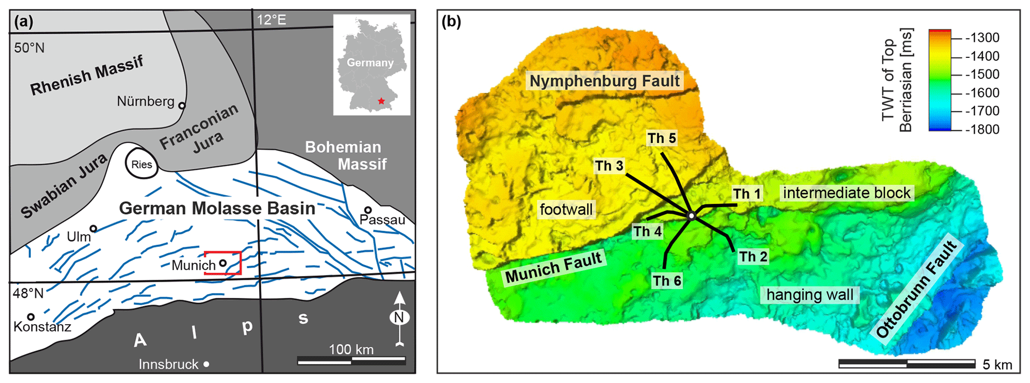
Figure 1Geological context and study area. (a) Simplified overview of the German Molasse Basin with tectonostratigraphic units and major faults (blue lines). The study area and the location of the GRAME 3D seismic are marked by a red star and rectangle, respectively. (b) Further input data are gathered from geophysical logging of the geothermal site Schäftlarnstraße (Sls) in the city of Munich, which contains six horizontally deviated wells (Th1 to Th6). Based on the horizon interpretation of the 3D seismic data carried out by Ziesch (2019), the Upper Jurassic reservoir is located at a depth between 1380 and 1750 ms TWT or around 1750 to 2600 m depth below sea level.
2.1 Geological evolution
The German Molasse Basin (GMB) is part of the North Alpine Foreland Basin, which experienced a complex structural evolution with a Permo-Carboniferous graben phase, a Triassic to Middle Jurassic epicontinental or shelf phase, a Middle Jurassic to Cretaceous passive margin phase, and a Tertiary foreland phase (Bachmann et al., 1987; Bachmann and Müller, 1992). During the Upper Jurassic, up to 600 m of carbonate, partly forming reef buildups, was deposited in the study area, which at that time was covered by the Tethys Sea (Schmid et al., 2005; Pieńkowski, 2008). At the Jurassic–Cretaceous boundary, regression of the Tethys led to the exposure of the carbonate deposits and caused strong karstification (Bachmann et al., 1987; Bachmann and Müller, 1992). Several isolated sinkholes and also sinkhole clusters can be observed at fault terminations or within the reservoir (Lemcke, 1988; Ziesch, 2019; Wadas and von Hartmann, 2022). From the Late Cretaceous to early Tertiary, southern Germany was uplifted, resulting in extensive compressional deformation due to the Alpine Orogeny. As a result, antithetic and synthetic normal faults developed parallel to the Alpine front (Ziegler, 1987). Furthermore, the underthrusting of the European plate below the Adriatic–African plate in the Late Eocene caused the Alpine nappes to extend to the north, which led to isostatic-induced downflexing of the GMB (Frisch, 1979). The development of the GMB was accompanied by two major transgressive–regressive cycles (Eisbacher, 1974), each causing the accumulation of marine deposits followed by terrestrial sediments, e.g. from rivers and lakes known as “marine molasse” and “freshwater molasse”, respectively. Finally, the molasse sediments were overlain by Pleistocene glacial and interglacial deposits.
2.2 Geothermal reservoir
The southward-dipping Upper Jurassic carbonates (Malm) form a carbonate platform which is the geothermal reservoir (Schmid et al., 2005; Pieńkowski, 2008). Due to the southward increase in depth, the temperatures increase towards the south from approximately 70 to 150 ∘C. This allows extraction of geothermal energy for heating in the Munich area and even electricity generation further south (Böhm, 2012; Agemar et al., 2014; Homuth et al., 2015).
With regards to the depositional system, the Malm of the greater Munich area can be separated into two hyper-facies: a massive facies (consisting of reefs) and a bedded facies (Reinhold, 1998; Machel, 2004; Lucia, 2007; Bohnsack et al., 2020). Several studies have shown that reefs are suitable exploitation targets because they are often prone to dolomitization, karstification, and brittle deformation, and therefore they often exhibit enhanced groundwater flow (Andres, 1985; Stier and Prestel, 1991; Birner et al., 2012). A lithofacies-based hydrostratigraphic classification for the greater Munich area carried out by Böhm (2012) shows that the lowermost units Malm α to Malm γ, which mainly consist of marly limestones, can be characterized as an aquitard. Malm δ to Malm ϵ are described as a regional aquifer due to a laterally persistent dolomitic massive facies. Malm ζ contains local aquifers in dolomitized massive facies as well as aquitards.
Structural analysis of the GRAME 3D seismic dataset reveals that the study area is influenced by karstification and fault-related deformation. Several isolated sinkholes and also sinkhole clusters are observed along the fault traces and at fault terminations (Sell et al., 2019; Ziesch, 2019; Wadas and von Hartmann, 2022). The seismic data also show that the greater Munich area is traversed by a complex fault pattern, mainly consisting of normal faults. The largest fault with a maximum vertical offset of 350 m is the Munich Fault (Fig. 1b), which splits eastward into several branches that subdivide the area around the geothermal site “Sls” into a footwall block, an intermediate block, and a hanging-wall block. The large fault system in the southeast is the Ottobrunn Fault that also splits into several small antithetic and synthetic faults with small vertical offsets up to 80 m, forming a horsetail splay. This indicates this fault has both normal fault- and strike-slip components (Ziesch, 2019). Overall, the Upper Jurassic carbonates of the Munich area are characterized as a strongly heterogeneous, lithology- and facies-dependent, fracture- and karst-controlled reservoir (Birner et al., 2012; Cacace et al., 2013; Homuth et al., 2015; Moeck et al., 2020).
3.1 Database
For better insight into the structure and diagenesis of the reservoir, we performed an advanced seismic data analyses of the GRAME dataset using the seismic interpretation software Schlumberger Petrel®. The GRAME 3D seismic dataset, which was surveyed and processed in 2015–2016 by DMT Petrologic GmbH (Maximilian Scholze and Florian Wolf, personal communication, 2016), had variable line distances of 400 to 500 m and a source and receiver spacing of 50 m with a sweep frequency of 12 to 95 Hz, 5 s of record length, and a 2 ms sample rate. This configuration enabled the acquisition of a high-resolution 3D cube with a good signal-to-noise ratio. The seismic data processing consisted e.g. of static corrections, deconvolution, common reflection surface (CRS) analysis, migration velocity analysis based on tomographic inversion, and Kirchhoff pre-stack depth migration (for details see the tabular overview in Wadas and von Hartmann, 2022, and the acquisition and processing reports by Maximilian Scholze and Florian Wolf, personal communication, 2016). Based on these data, we performed an advanced seismic data analysis comprised of single- and multi-attribute analysis. Furthermore, an attribute and neural-network-based lithology classification and an ant-track-based seismic fracture orientation analysis were carried out. For this purpose, we implemented datasets of the six Schäftlarnstraße wells, which were geologically and geophysically investigated. The well logging was carried out in 2018–2019 by the company Daldrup & Söhne AG on behalf of the Stadtwerke München (SWM). The available data include stratigraphic and lithological information from cuttings (Franz Böhm and Matthias Dax, personal communication, 2019) and image logs (Stadtwerke München, personal communication, 2019). The drill cuttings were used to determine the dolomite and calcite content at intervals of 2.5 to 5 m by calcimetry in order to derive a lithology log. The image logs show the electrical resistivity of the borehole walls and allow for a classification of different rock types and fractures (e.g. Schlumberger, 2004; Böhm, 2012; Lai et al., 2018).
3.2 Seismic single-attribute analysis
Seismic attributes are quantities computed from the seismic data and describe the shape or physical characteristics of one or more seismic traces, mostly over specified time intervals. The characteristics of a seismic wave, e.g. velocity, amplitude, frequency, phase, and attenuation, change while the wave propagates through the subsurface. These changes are caused by the different physical rock properties of the various rocks in the subsurface. Therefore, they are used to highlight specific geological, physical, and/or reservoir properties and to help recognize patterns and parameter relationships (Taner, 2001; Chopra and Marfurt, 2007; Veeken, 2007). Seismic single attributes can be categorized by different taxonomies (Dewett et al., 2021). In this work, we group them by the properties they measure, namely amplitude-related attributes, phase- and frequency-related attributes, and discontinuity-related attributes. See the Appendix for more detailed information regarding the seismic attributes and the chosen parameters for the attribute analysis.
3.2.1 Amplitude-related attributes
These attributes (e.g. root mean square – rms – amplitude, envelope, reflection intensity, and acoustic impedance) are used to depict stratigraphic and lithologic contrasts. The rms amplitude is described as the square root of the sum of squared amplitudes divided by the number of samples within a specified time window. The reflection intensity is the average amplitude over a specified time window multiplied by the sample interval. And the envelope is the magnitude of the complex trace and is independent of phase (Chopra and Marfurt, 2007; Sarhan, 2017). These three attributes mainly identify only strong anomalies (see Fig. A1), and to depict smaller variations, as expected in our study area, we also used acoustic impedance. Every reflection changes the amplitude of the returning wave due to a contrast in acoustic impedance, which is the product of the seismic velocity of the wave travelling through the subsurface and the density of the rock. Therefore, the reflection amplitudes can be inverted to get impedance values (Pendrel, 2001; Barclay et al., 2008; Filippova et al., 2011) by using e.g. a stochastic seismic amplitude inversion, as carried out in this study area by Wadas and von Hartmann (2022).
3.2.2 Phase- and frequency-related attributes
Phase- and frequency-related attributes (e.g. instantaneous phase, instantaneous frequency, and dominant frequency) show the continuity of weak reflectors and indicate unconformities, faults, fracture zones, lithology and stratigraphic sequences, and sequence boundaries (Van Tuyl et al., 2018). The instantaneous phase measures the phase shift of a specific reflection event, e.g. resulting from a polarity reversal of the reflection coefficient or due to a curved interface (Chopra and Marfurt, 2007). The instantaneous frequency is the rate of change of the instantaneous phase, and the dominant frequency is the square of the instantaneous frequency summed with the square of the instantaneous bandwidth, and then the square root of the sum is calculated (Schlumberger, 2020). So the dominant frequency indicates where the energy of the seismic signal is concentrated in the frequency domain.
3.2.3 Discontinuity-related attributes
Such attributes (e.g. variance and chaos) are able to image vertical and lateral discontinuities and can therefore highlight stratigraphic and structural boundaries like faults, fractures, dolines, and reef edges (Chopra and Marfurt, 2007). For the variance, a trace-by-trace analysis is performed in order to quantify the dissimilarity of the seismic waveform of neighbouring traces within a specified time window (Bahorich and Farmer, 1995; Marfurt et al., 1998; Wang et al., 2016). Chaos is a similar attribute that maps the “chaoticness” of the seismic signal from statistical analysis of dip and azimuth estimates.
3.3 Seismic multi-attribute analysis
The complexity of carbonates makes combined analyses of several different attributes necessary in order to characterize and better understand the reservoir. In a multi-attribute analysis, several single attributes, which are mathematically independent but linked through the underlying geology, can be combined by co-rendering and colour blending or by using them to calculate new attributes (Marfurt, 2015). Since a good seismic attribute should represent important aspects of the underlying geology, showing more than one attribute in the same image can give improved geological insight. See the Appendix for more detailed information regarding the seismic attributes and the chosen parameters for the attribute analysis.
3.3.1 Sweetness
Sweetness can enhance the visibility of lithological and structural changes (Chen and Sidney, 1997). It is the mathematical combination of instantaneous frequency and envelope (Radovich and Oliveros, 1998), and the combination of these two attributes is able to detect general energy changes in the seismic wave. High sweetness values are correlated with both high envelope and low instantaneous frequencies, whereas for low sweetness values it is the opposite.
3.3.2 Spectral decomposition
Spectral decomposition is a useful tool for qualitative and quantitative interpretation because it allows delineating geological features in more detail due to tuning at a specific frequency (Henderson et al., 2008; Wang et al., 2016). Therefore, it can enhance subtle structural features, like thin beds, reefs, channels, and pinch-outs (Chopra and Marfurt, 2007; Marfurt and Kirlin, 2001; Marfurt, 2015), and it can also be used for seismic geomorphology analysis (Marfurt and Kirlin, 2001). In principle, spectral decomposition (Fig. A2) separates the seismic signal into its frequency components. Three different frequencies are then co-rendered and displayed by RGB colour blending, where frequencies 1, 2, and 3 are plotted as red, green, and blue, respectively (Chopra and Marfurt, 2007; Al-Maghlouth et al., 2017).
3.3.3 Curvature
Curvature is used to detect changes in depositional and geological trends, e.g. tectonic features and lineaments. Therefore it is useful to identify e.g. channels and valleys, karst and dolines, and mounds and reef buildups (Al-Dossary and Marfurt, 2006). Curvature measures how much a seismic reflector is bent. In the case of a planar reflector, the corresponding vectors are parallel and the reflector has zero curvature. In contrast, anticlinal features result in diverging vectors and the curvature is positive. Synclinal features result in converging vectors and the curvature is negative (Roberts, 2001; Al-Dossary and Marfurt, 2006; Wang et al., 2016). The most positive (Kpos) curvature and most negative (Kneg) curvature are often co-rendered and used for morphological analysis (Chopra and Marfurt, 2007; Marfurt, 2015).
3.3.4 Shape index and curvedness
Additionally, curvature can be used to calculate new attributes such as the shape index and the curvedness that allow a quantitative definition of the local morphology of a seismic reflector or seismic horizon, independent of scale (Roberts, 2001; Chopra and Marfurt, 2007; Veeken, 2007; Wang et al., 2016; Sarhan, 2017). The shape index describes the type of shape of a specific surface, and the index differentiates between dome (+1), ridge (+0.5), saddle (0), valley (−0.5), and bowl (−1) shapes (Chopra and Marfurt, 2007; Marfurt, 2015). The curvedness measures the magnitude of curvature, which is zero for a planar surface (Roberts, 2001). Both attributes are often co-rendered together with variance or chaos to visualize reflector morphology (Marfurt, 2015).
3.4 Neural-network-based lithology classification
The lithology classification in this study is based on a rock physics workflow, which predicts the most probable lithologies utilizing an artificial supervised neural network using the software Schlumberger Petrel®. 3D seismic volumes, well logs, and geological interpretations can serve as input datasets. At first, a class definition (class 1: limestone, class 2: dolomitic limestone, class 3: dolomite, class 4: calcareous dolomite) using well logs is carried out, after which the classification algorithm can be generated and finally used for lithology prediction (Schlumberger, 2020).
To obtain input parameters for the neural network, we tested whether relationships exist between the lithology classes and the physical parameters derived from the seismic attributes. This was accomplished by cross-plotting the lithology logs from the six wells against the seismic attributes that were extracted from the 3D volumes along the well paths. A correlation analysis was carried out, and the correlation coefficients between the lithology classes and the attributes were determined. Based on the results, the following attributes were chosen: acoustic impedance, dominant frequency, reflection intensity, variance, envelope, and the 28 Hz frequency band; then a cluster analysis was carried out to develop a classification algorithm. This cluster analysis was performed by utilizing a supervised artificial neural network (ANN), which automatically searched for the best relationships between the seismic attribute values and the lithology classes. The ANN is a type of computational model, which tries to mimic pattern recognition and data interpretation of the human brain (Da Silva, 2017). The supervised ANN is trained with both the input data (seismic attribute “logs”) and the desired output data (lithology logs). The network architecture consists of an input layer, a hidden layer, and an output layer. The input layer consists of input neurons also called nodes and takes the input data, in our case the seismic attribute data, and passes them to the hidden layer. In the hidden layer, the ANN learns the relationship or connection between the different nodes and the output values by applying weight functions between them. Then the sum of all weighted inputs is calculated and the output layer gives the predicted output values of the ANN (Da Silva, 2017). In our case, these output values are the four carbonate classes. From this neural-network-based cluster analysis, 2D and 3D probability density estimates were derived (Fig. 2a and b). Training the estimation model and neural net was an iterative process, and at the end of each iteration the training error was calculated. The error was assessed by comparing the neural network result with the desired output, in this case the lithology logs. At the beginning, the training data were split into two parts; one part was used for the training and the other was used to calculate the error by cross-validation (Schlumberger, 2020). The chosen ratio was 50:50, so 50 % of the data were used for training of the neural network and the other 50 % were used to cross-validate the results. To quality-control the performance of the classification algorithm a confusion matrix was generated (Fig. 2c). It allows the user to identify whether the algorithm became confused when defining the different classes (Sammut and Webb, 2017). The upper confusion matrix shows the probability of a classification occurring given the true class. The rows contain the true classes and the columns contain the predicted classes. For example, 8.18 % of the samples that belong to the limestone class were wrongly predicted as dolomite, and 86.17 % of the samples that belong to the dolomite class were correctly predicted as dolomite. The lower confusion matrix shows the data the other way around. High-confidence classification results have large values along the diagonal of the matrix, as is the case in our study, indicating a reliable classification result. Furthermore, the data quality was also visually inspected by comparing the actual lithology logs from the six wells with estimated logs based on the neural network, and it also shows a good classification result (Fig. 2d). The successfully trained neural net was then used to create a 3D model with the predicted lithologies based on the 3D seismic attribute volumes (Schlumberger, 2020).
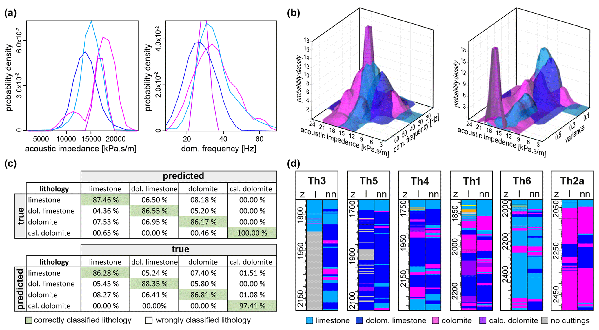
Figure 2Lithology classification using a supervised neural network based on parameter relationships between the input data (e.g. seismic attributes) and the desired output data (e.g. lithology classes from logs). (a–b) After choosing appropriate seismic attributes for the classification, these attributes were used to create probability density estimates, e.g. in 2D and 3D (exemplarily shown for acoustic impedance, variance, and dominant (dom.) frequency). The results of the lithology classification were validated by examining (c) a confusion matrix table and (d) a comparison between the actual lithology log (l) and the predicted lithology log (nn) derived from the neural net. The upper confusion matrix table shows the probability of a classification occurring given the true class. The lower confusion matrix table shows the probability of a sample belonging to a particular class given the predicted class. A reliable classification with high confidence has large values along the diagonal of the matrix (marked in green).
3.5 Ant-track-based fracture orientation analysis
Several studies have shown the applicability of 3D seismic data for fracture analysis (Jaglan et al., 2015; Fang et al., 2017; Albesher et al., 2020; Boersma et al., 2020; Loza Espejel et al., 2020; Méndez et al., 2020), which can be used to address the often-raised question of scalability of reservoir properties (e.g. Lake and Srinivasan, 2004; Li et al., 2019); i.e. can information regarding fracture properties be transferred from the well scale to the seismic scale and vice versa? To address this question, an adapted seismic fracture orientation analysis (FOA) workflow based on e.g. Albesher et al. (2020) and Boersma et al. (2020) was applied. Afterwards the FOA results on the seismic scale were compared with those on the image log scale.
The FOA workflow, based on the 3D reflection seismic volume, consisted of several steps, starting with the extraction of an edge-detection volume, in this case variance (Fig. 3 – step 1), which images lateral and vertical discontinuities (Marfurt et al., 1998; Chopra and Marfurt, 2007). Then the edge evidence attribute was applied to enhance the edges and thus the fractures in the variance volume (Fig. 3 – step 2). The edge evidence attribute searches for segments in which the variance values differ significantly from the surrounding values in order to enhance them (Schlumberger, 2020). Afterwards Schlumberger's patented ant-tracking algorithm (Schlumberger, 2020) was applied (Fig. 3 – step 3). Ant tracking can be used to extract faults and fractures from a discontinuity volume. This is accomplished by simulating the behaviour of ants, which use pheromones to optimize their search for food by marking their paths. Following the same principle, artificial ants (agents) are used to search for faults and fractures, generating a detailed attribute volume with very sharp edges. A choice can be made between a passive and an aggressive ant-tracking mode, and since our investigation focus is on small structures like fractures and not large structures such as faults, we chose an aggressive mode and adapted its parameters to our data (see additional explanation in the Appendix). After the first ant tracking a second ant tracking was applied to further sharpen the detected edges (Fig. 3 – step 4). Afterwards automatic fracture extraction (Schlumberger, 2020) was used to create 3D fracture patches from the ant-tracked volume (Fig. 3 – step 5). Then the fractures from the patch volume were extracted along the well paths, including an area with a diameter of 1 km around each well, in order to capture enough fractures for the analysis (Fig. 3 – step 6). Afterwards, visual quality control was carried out and fracture patches that deviated from the ant tracks were manually removed from the dataset (Fig. 3 – step 7). The fracture patches along the well paths (Fig. 3 – step 8) and their corresponding fracture orientation values were then exported from Petrel and imported into the software Stereo32 to create rose diagrams and stereogram pole plots in order to analyse the fracture orientations and to determine fracture clusters. Subsequently, the results were compared for the complete drill paths and sections of it with those of image log analyses to show where the fractures matched. The compact micro-imager (CMI) images the rock's electrical resistivity and is presented as an unrolled figure of the well surface (Schlumberger, 2004). Since fractures have a different resistivity compared to the surrounding rock, they are visible as sinusoids. We traced their orientation manually by using the software WellCAD (ALT, 2021). The image is referenced according to the well path so that the software calculates the true orientation of the fractures.
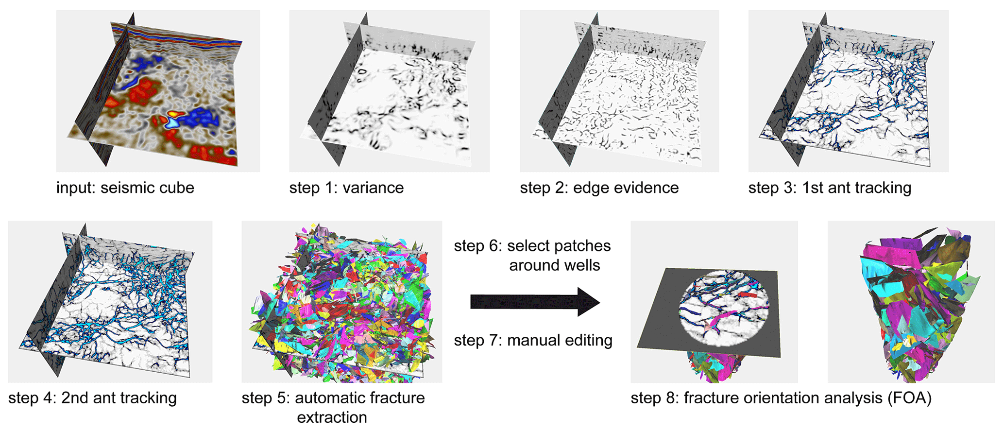
Figure 3Fracture orientation analysis workflow, shown on a zoomed-in section of the GRAME dataset, based on seismic attributes and ant tracking.
In the following, the results of the physical and structural reservoir characterization, the lithology prediction model, and the fracture orientation comparison are shown. Please note that the carbonate formations of the GMB generally dip to the south, and additionally, our study area shows a fault-related downward-stepping to the south. Therefore, the carbonate deposits on the footwall of the Munich Fault are located at shallower depths and time slices compared to the hanging wall.
4.1 Physical and structural reservoir characterization
4.1.1 Geological main targets
In the GRAME area, several of the main exploration targets can be identified based on the acoustic impedance volume, e.g. reef buildups and dolines, as described by Wadas and von Hartmann (2022). For example, in the west of the footwall block, an elongated reef (Fig. 4a) with high impedance values of up to 18 000 kPa s m−1 in the reef core and low impedance values down to around 10 000 kPa s m−1 at the reef margins can be seen. Comparable characteristics are observable for another reef in the east of the intermediate block (Fig. 4b).
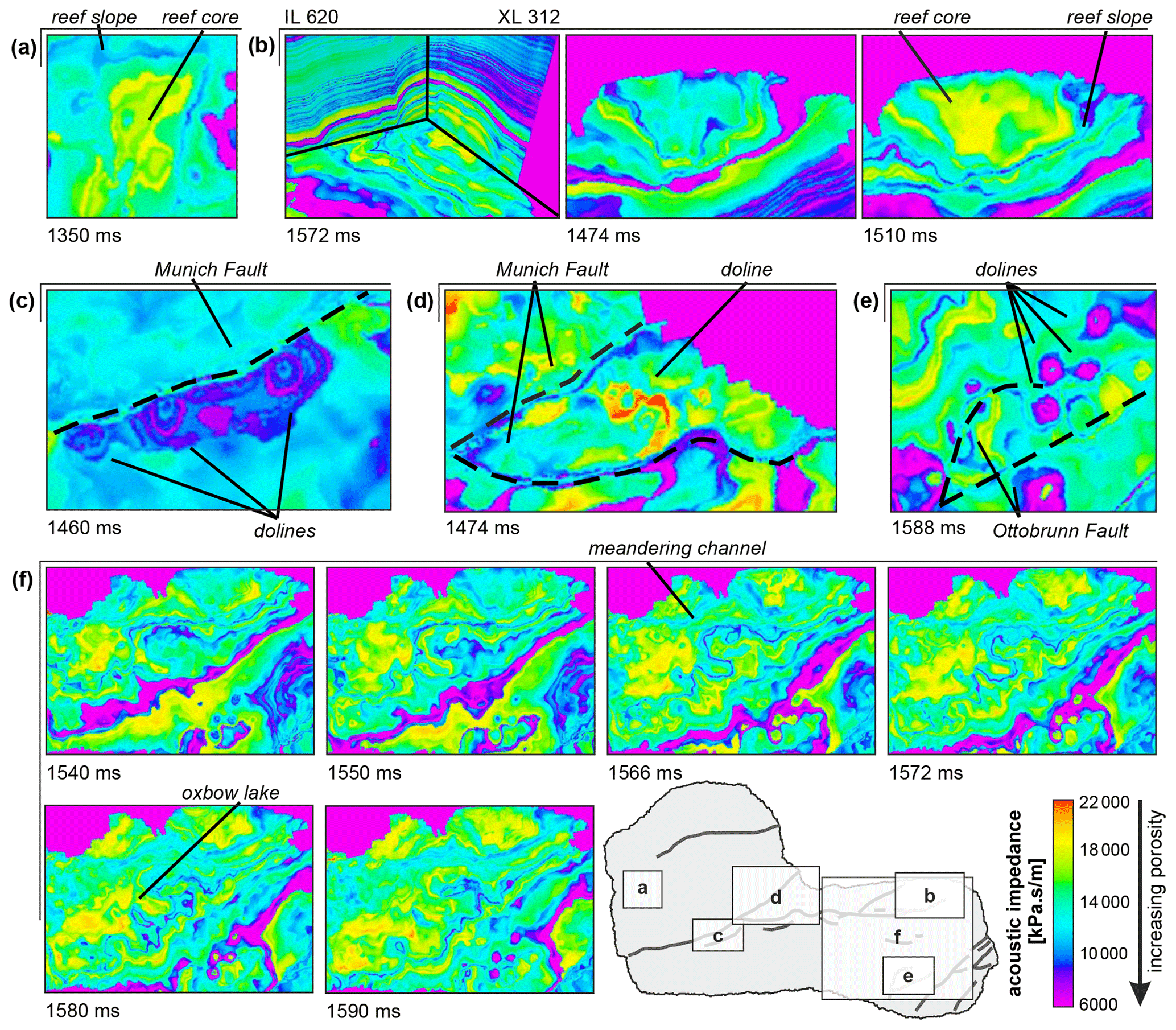
Figure 4Time slices through the acoustic impedance volume, calculated by Wadas and von Hartmann (2022), which is used to depict stratigraphic and lithological contrasts. The results reveal impedance contrasts of different carbonate structures associated with a shallow-marine environment and sea level variations, such as reef buildups (a–b), karst features (c–e), and a channel (f). Low impedance values correlate with high porosities. IL: inline, XL: crossline.
The identified dolines are typically characterized by a circular shape. In the study area, large dolines and doline clusters are often located close to faults. This is because the fracture zones around faults can lead to enhanced fluid migration and therefore increased dissolution of soluble rocks and the development of secondary porosity, as can be observed e.g. at the Munich Fault (Fig. 4c, d) and the Ottobrunn Fault (Fig. 4e). The dolines have low impedance values in the centre and often larger impedance values around them. Another observed feature is an incised narrow channel in the upper reservoir part in the east of the hanging wall, crossing the area from northeast to southwest (Fig. 4f). This channel is associated with a low-stand sea level and subaerial exposure of carbonates. The channel fill is clearly visible due to its low impedance values, which show a strong contrast compared to the impedance of the surrounding rocks. In the deeper time slices, e.g. at 1590 ms, the channel is only slightly curved and follows a more or less straight northeast–southwest direction. Over time, the channel started to meander (e.g. at 1580 and 1572 ms), also resulting in the development of oxbow lakes. A derived porosity model based on an impedance–porosity relationship, which associates low impedance values with higher porosities, shows a complex porosity distribution within the study area (Wadas and von Hartmann, 2022). The reef core has porosities mainly <3 %, and the highest porosities of 7 % to 14 % are observed at the reef cap, in the upper third of the reef, and on the reef slopes. Wadas and von Hartmann (2022) assume that this is the result of intense karstification and gravitational mass flows on the slopes. Overall, the footwall of the Munich Fault shows higher porosities than the hanging wall to the south, and the porosity also displays a W–E trend with higher porosities in the western part of the study area. Furthermore, based on a comparison of their results with well data, they describe dolomitic limestone as having the highest porosities and calcareous dolomite the lowest porosities. Thus, preferential exploitation targets in terms of high porosity are more likely to be found in the upper part of the reservoir (Berriasian to Malm ζ1), in particular in dolomitic limestones due to their high porosity and/or in strongly karstified areas within bedded and reef facies.
Besides amplitude and impedance, other physical properties describing the signal of a reflected seismic wave are phase and frequency. In our study area noticeable changes in seismic phase are observed at interface boundaries of dolines and reefs. In addition to the already identified dolines and doline clusters (Fig. 4), we found smaller circular features in the north of the footwall which were also interpreted as dolines (Fig. 5a). The already identified dolines at the Munich Fault (Fig. 5b) and at the Ottobrunn Fault (Fig. 5c) also produce clear phase changes in the seismic signal. Furthermore, two additional circular features can be seen north of the already identified doline cluster at the Ottobrunn Fault. Phase changes are also observed at reef boundaries and within the reefs. For example, the reef to the east of the intermediate block (Fig. 5d) shows a clear phase change at the outer reef edge, but internally, further phase changes can be observed, in part almost parallel to the outer edge, whereas in the centre, there is an area with a laterally almost constant phase, e.g. at 1470 ms. This is the reef core; the surrounding phase changes reflect the shifting of the reef edge and thus the reef growth that has led to the enlargement of the reef over time. Furthermore, at the southeastern edge of this reef, the areas of the same phase sometimes have a significantly smaller lateral extent than at the southwestern edge, e.g. at 1490 and 1500 ms. This indicates that in the southwest of the reef the same lithology or facies occupies a larger spatial area than in the southeast. Thus, we assume that this reef has either not uniformly spatially grown or was affected by spatially uneven erosion due to e.g. spatial differences in water motion, sediment dynamics, and/or subaerial exposure.
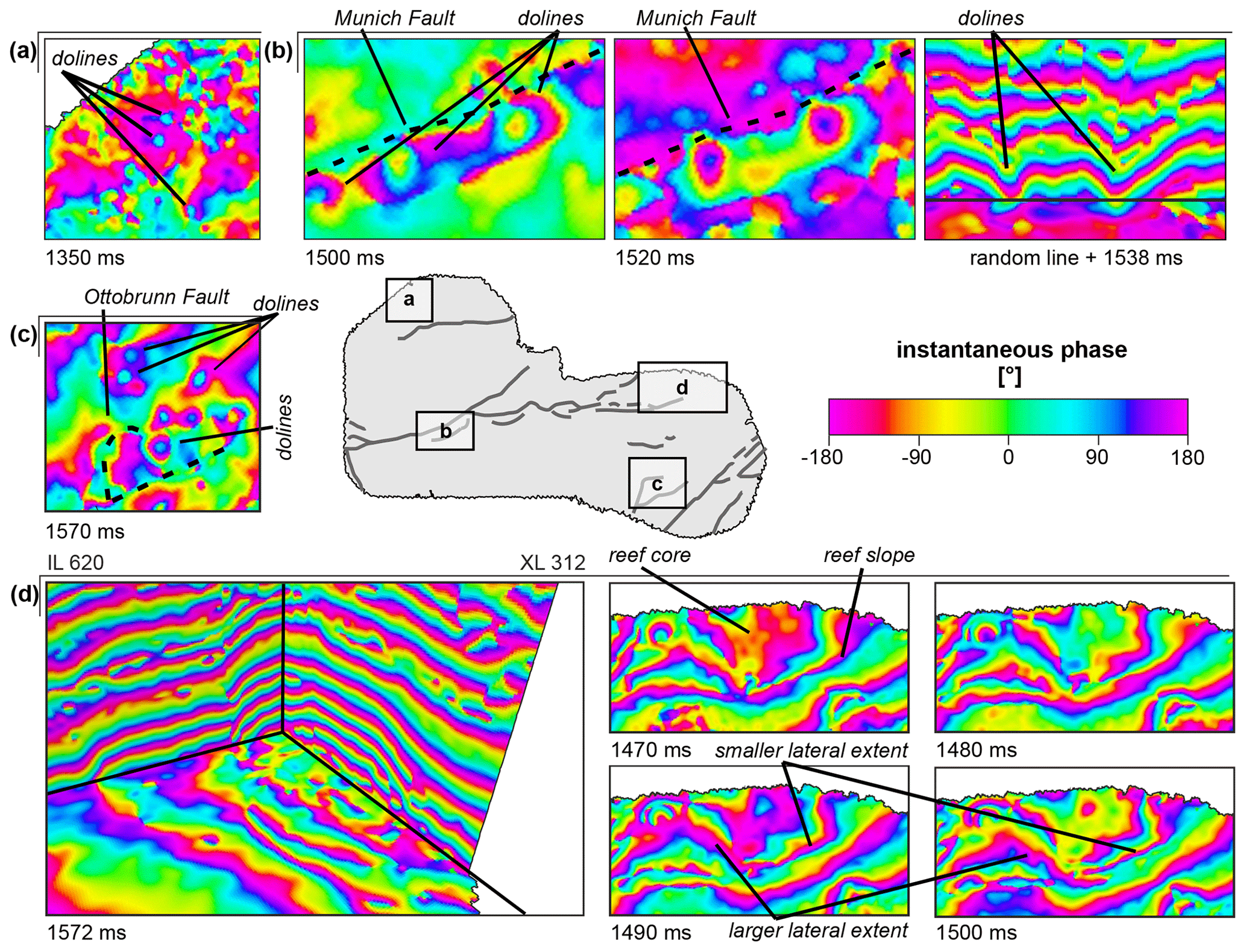
Figure 5Time slices through the instantaneous phase volume, which is used to identify phase shifts in the data. Strong phase changes, independent of amplitude, are observable at structural and interface boundaries, e.g. dolines (a–c) and reefs (d). IL: inline, XL: crossline.
With regard to the investigation of the dominant frequencies in our study area, it has been shown that the frequencies are mostly below 40 Hz, indicating strong frequency attenuation. Nevertheless, the degree of frequency attenuation differs, even for the same type of structural feature. For example, a reef buildup in the west of the hanging wall (Fig. 6a) shows much lower dominant frequencies of mostly less than 20 Hz compared to the reef in the east of the intermediate block (Fig. 6b) with frequencies of mostly around 20 to 40 Hz. For the latter, only the reef slopes and the cap have frequencies below 20 Hz. This correlates with the results of the impedance analysis, which show that these zones are characterized by lower impedance values and therefore higher porosities (Fig. 4a and b). This might result from mass redistribution at the slopes and more intense karstification leading to stronger attenuation of higher frequencies. For the reef in the west of the hanging wall, this means that it might be more karstified. The correlation of karstification and low frequencies is also observable for the large dolines at the Munich Fault (Fig. 6c) and the Ottobrunn Fault (Fig. 6d). The doline margins are characterized by very low frequencies of mostly below 20 Hz, while the doline centre shows slightly higher frequencies of around 25 to 30 Hz. As shown by other doline studies, their margins are often strongly fractured (e.g. Waltham et al., 2005; Al-Halbouni et al., 2018; Wadas et al., 2018), leading to a loss of high frequencies. Besides reefs and karst, the filling of the narrow channel, identified in the impedance volume, is also characterized by lower frequencies compared to the surrounding material (Fig. 6e), although the frequencies differ along the channel, indicating variation of the channel fill.
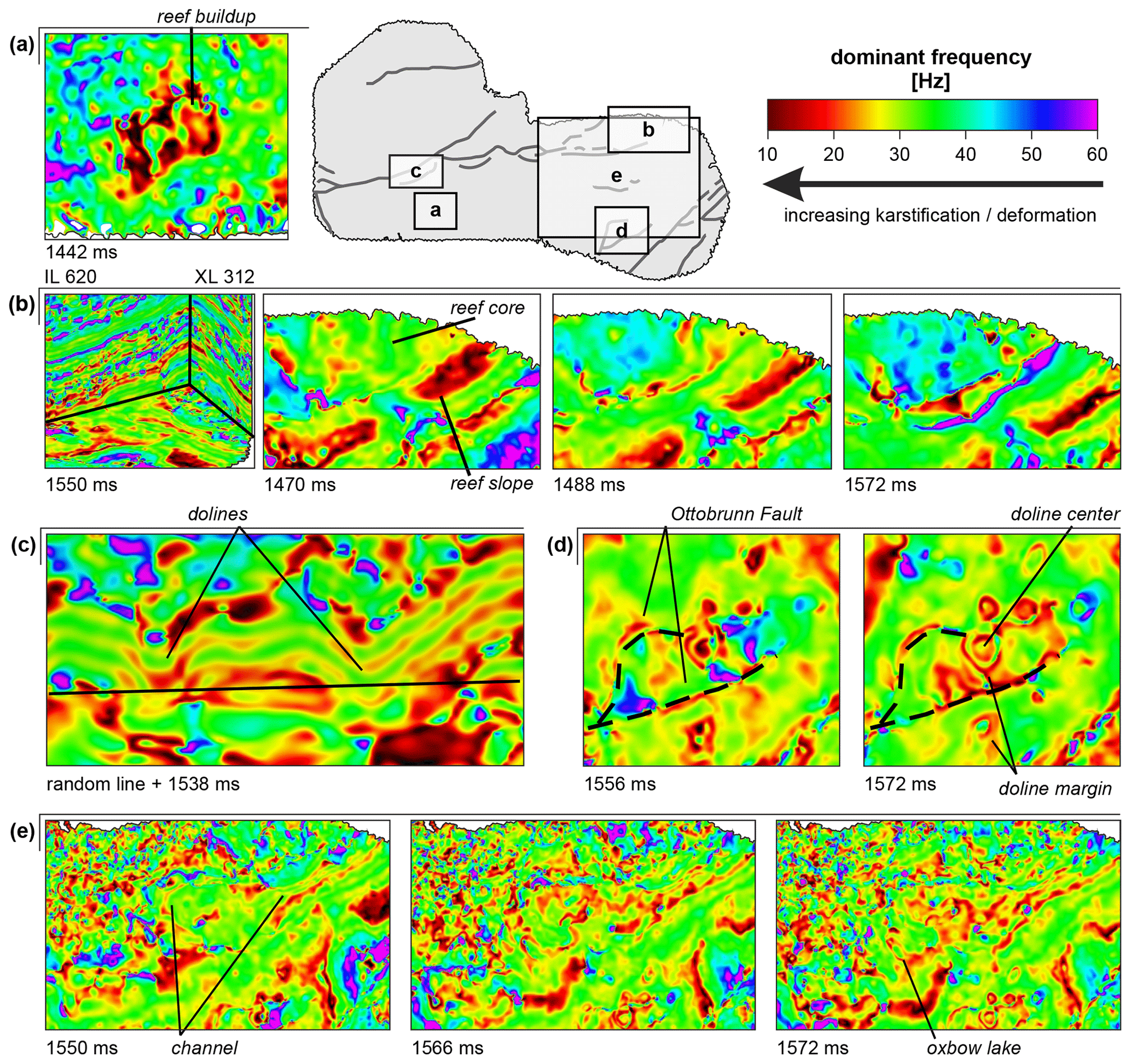
Figure 6Time slices through the dominant frequency volume showing the varying frequency attenuation across the study area, e.g. (a–b) within reefs, (c–d) dolines, and (e) channels. Lower dominant frequencies indicate increased karstification and/or fault-related deformation. IL: inline, XL: crossline.
Another way to analyse the frequency content of a seismic dataset is by spectral decomposition because the examination of individual frequency components enables better spatial differentiation and correlation. The reef buildups, the karst features (dolines and widespread dissolution along bedding planes), and also the meandering channel are all characterized by mainly low frequencies of 18 Hz and partly high frequencies of 50 Hz, represented by red, pink, and to a lesser degree purple (Fig. 7). This frequency attenuation due to scattering at e.g. fractures and reef edges could be caused by intensive karstification and mass redistribution. In addition, lithological variations can also lead to frequency differences. Regarding regional trends, the footwall of the Munich Fault (Fig. 7a) shows a north–south differentiation towards the deeper time slices. The northern part of the footwall is mainly dominated by the 28 Hz frequency component and partly by the 50 Hz frequency component, which is represented by green and green-blue. The southern part of the footwall is characterized by increasingly lower frequencies towards deeper time slices; at 1358 ms all three frequency components are present, at 1380 ms the 28 Hz component dominates together with the 18 Hz component, and at 1396 ms the 18 Hz band dominates. The upper part of the hanging wall of the Munich Fault (Fig. 7b) shows a west–east frequency differentiation. The western part contains mostly the 18 Hz and partly the 50 Hz frequency components, and only at greater depths is the 28 Hz component also present. To the east, a bright-coloured area can be seen, e.g. at 1524 and 1544 ms, indicating that all three frequency components are present and no general loss of high and/or low frequencies occurs. Overall, the hanging wall of the Munich Fault is more dominated by the blue 50 Hz frequency band than the footwall; the only exception for the hanging wall is the easternmost area containing the Ottobrunn Fault, which shows lower frequencies.
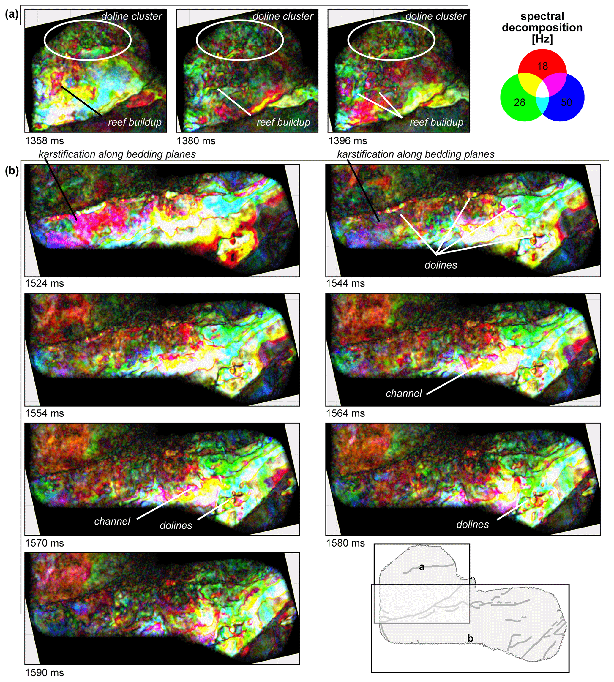
Figure 7Time slices through the spectral decomposition volume with 18 Hz plotted against red, 28 Hz plotted against green, and 50 Hz plotted against blue. It enables the examination of individual frequency components, showing spatial frequency variations (a) on the footwall and (b) on the hanging wall of the Munich Fault.
4.1.2 Internal reef architecture
To investigate the internal reef architecture, the seismic multi-attribute sweetness was analysed. In our study area, the bedded facies is characterized by low sweetness values (brown, dark blue, and grey), indicating a low envelope and high frequencies (Fig. 8). In contrast, the reefs that show a strong variation in sweetness are characterized by a higher sweetness due to increased envelope values compared to the surrounding material. The reef base (Fig. 8a – 1462 ms) and parts of the reef core show very high sweetness values (white, light blue, and yellow). This results from very high envelope values combined with relatively low frequencies. Such a combination of envelop and frequency could indicate a mudstone or a generally compacted and cemented (fine-grained, microcrystalline) limestone (Dunham, 1962; Flügel, 2010). The reef core has medium to high sweetness values resulting from medium envelope values and low to medium frequency values (Fig. 8; light green, pink, orange, medium blue, and red). This indicates a mixed mud- and grain-supported carbonate texture, which is typical of a reef core that consists of different types of biogenic components like sponges, bivalves, corals, and bryozoans surrounded by a matrix (Flügel, 2010; Böhm, 2012; Homuth et al., 2015). The different biogenic components cause variations in rock properties, such as rock density or seismic wave velocity, which result in stronger amplitude differences and lower frequencies due to increased attenuation. The reef slopes have medium sweetness values (dark green and purple), resulting from low frequency and low to medium envelope values. This corresponds to other studies which have shown that reef slopes often consist of a grain-dominated and strongly disturbed debris facies (Flügel, 2010; Playton et al., 2010), which will lead to low internal reflection coefficients and strong frequency attenuation. The sweetness attribute also allows a more detailed interpretation of the reef development.
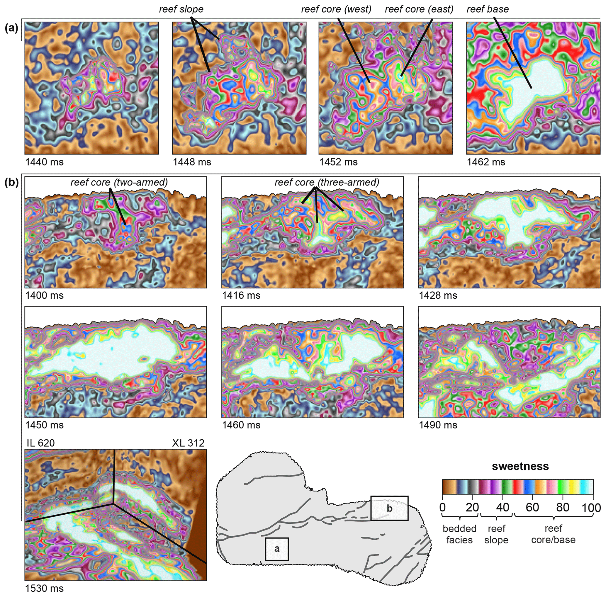
Figure 8Time slices through the sweetness volume, which detects general energy changes in the seismic wave in order to identify changes in lithology and stratigraphy. For the studied reservoir, the internal architecture of two exemplary reefs (a) in the west of the hanging wall and (b) to the east of the intermediate block of the Munich Fault is shown, revealing complex reef development. IL: inline, XL: crossline.
For example, in the case of the reef to the west of the hanging wall (Fig. 8a), we observe that, starting from the reef base at 1462 ms, two closely spaced but separate reef cores developed (1452 and 1448 ms), ultimately forming one large reef (1440 ms). The western reef core shows a bending orientation where the southern part has a SW–NE orientation and the northern part has SE–NW orientation, whereas the eastern reef core shows only a NW–SE orientation. In contrast, the reef to the east of the intermediate block (Fig. 8b) shows a slightly different development. The reef base, which is not shown, is spatially coherent, and also the reef core (from 1490 to 1460 ms) had a spatially mostly uniform development. However, in the upper part, at 1428 and 1416 ms, the reef core starts to develop the shape of a three-armed star with NNW–SSE, N–S, and NE–SW orientations. During further reef growth the NE–SW arm died out and only a NW–SE-oriented reef core remains (1400 ms). This change in reef core shape might result from a change in ocean currents or other local environmental changes.
4.1.3 Structural boundaries and lineaments
Variance and chaos are able to highlight structural boundaries and lineaments. However, both attributes deliver comparable results, so only the results of the variance analysis are shown. High variance values indicate high dissimilarities between neighbouring traces, especially on the footwall (Fig. 9a) and the intermediate block of the Munich Fault (Fig. 9b).
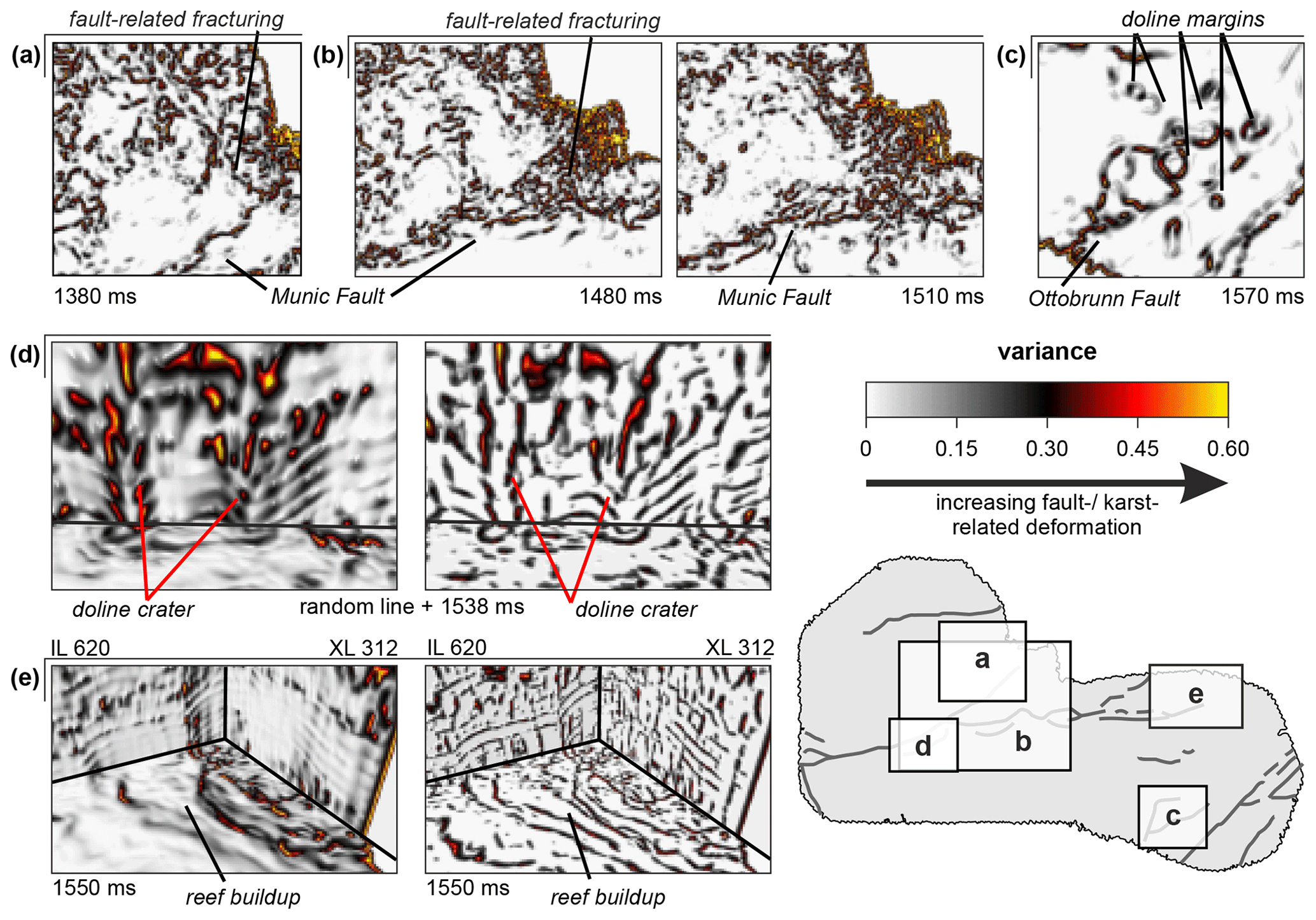
Figure 9Time slices through the variance volume, which is used to detect faults and fracture zones (a–b), karst features (c–d), or other structural features with sharp edges, such as reefs (e). In (d) and (e) the subpanels on the right show variance with an additionally applied edge-enhancement filter to better highlight the vertical discontinuities on an inline (IL), a crossline (XL), and a random line.
Long linear features and chaotic patterns are visible along the fault itself and in the surrounding areas, respectively. The former result from the strong discontinuities due to the fault displacement, and the latter are induced by fault-related deformation. Fault-related deformation can cause an increase in fracture intensity that generates more discontinuities, which is observable by high variance values. But discontinuities can also be caused by karst-related deformation, as can be seen, e.g. for the dolines at the Ottobrunn Fault (Fig. 9c) and the Munich Fault (Fig. 9d). In the top view, the strongly disturbed doline edge is shown by circular high variance values, and in the side view, the collapse crater is clearly visible due to vertical discontinuities. In addition, reef margins are also characterized by high variance values (Fig. 9e). These are presumably caused by mass redistribution due to debris flows at the margins, intensified karstification, and fracturing.
4.1.4 Morphological features
To analyse morphological features within the reservoir, we used the most positive curvature (Fig. 10a) and most negative curvature (Fig. 10b) co-rendered with variance (Fig. 10c). In our study area, the most positive curvature reveals many anticlinal features, and the most negative curvature reveals many synclinal features, as shown by an exemplary time slice at 1510 ms. Along the Munich Fault and its fault branches, long linear features can be seen (Fig. 10c). The positive curvature anomalies are associated with the upthrown side of the normal faults and the negative curvatures with the downthrown side (Roberts, 2001). The distance between the two anomalies gives an impression of the fault heave. Since the distance is quite small, this indicates a short lateral displacement of the fault, which also fits well with the finding that the faults in this study area are steeply dipping (Ziesch, 2019). Besides this, many small-scale lineaments that form a chaotic pattern are visible, especially on the intermediate block and the footwall. These small linear features are interpreted as fractures resulting from intense fault-related deformation along the Munich Fault, in particular within the area where the fault splits into two fault branches forming the intermediate block. Along this fault, but also along the Ottobrunn Fault to the south and within the fault blocks, many circular features can be seen, which are interpreted as karst-related dolines (Fig. 10d and e). The doline margins show a distinct positive anomaly indicating an anticlinal structure, whereas the doline centre shows a negative anomaly typical of a synclinal structure.
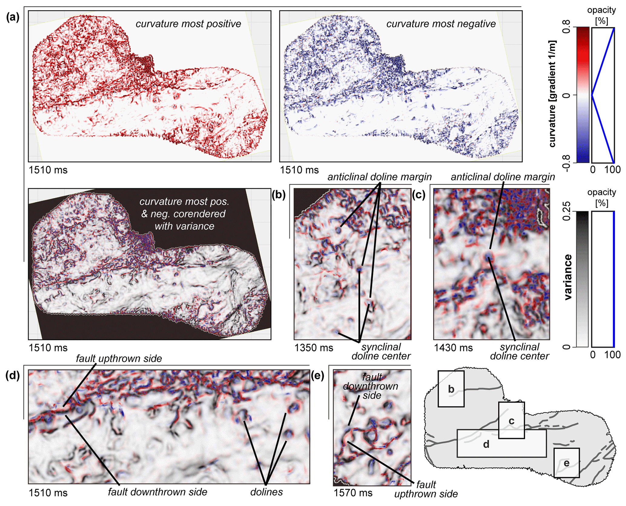
Figure 10Time slices through the curvature volumes that are utilized to detect changes in structural and depositional trends. (a) The most positive curvature reveals anticlinal features and (b) the most negative curvature synclinal features. (c) For a comprehensive interpretation both curvature volumes are superimposed and co-rendered with variance. The joint interpretation allows the detection of faults and the determination of the upthrown and downthrown sides, and it is also a suitable tool for doline detection (d–e).
Curvature distinguishes only between planar, anticlinal, and synclinal structures, but it can be used to calculate new attributes, such as the shape index and the curvedness (Fig. 11) that allow a quantitative definition of the local morphology (Roberts, 2001). Therefore, we co-rendered the shape index with curvedness and variance. In our study area, zones with planar or almost planar features, shown by dark grey, are observable on the hanging wall of the Munich Fault. Zones with highly curved morphologies, visible by bright colours, are seen on the footwall and the intermediate block of the Munich Fault and to the south at the Ottobrunn Fault, e.g. at 1510 ms (Fig. 11a).
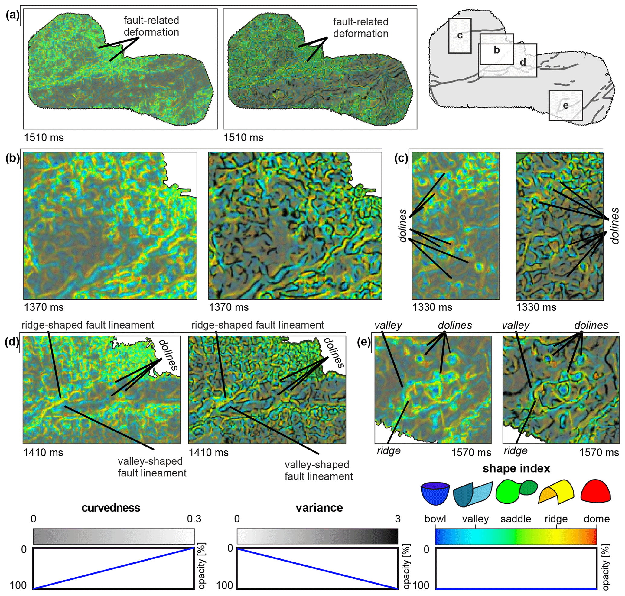
Figure 11Time slices through the co-rendered shape index and curvedness volumes (left panels), also together with the variance volume (right panels). The shape index describes the type of shape of a specific surface, and the curvedness measures the magnitude of curvature. Together with variance they are suited to visualize morphology (Marfurt, 2015), e.g. (b) damage zones, (c, e) karst-related dolines, (d, e), and faults.
The tectonically deformed fractured area in the east of the footwall block is characterized by a chaotic pattern of mainly ridge- and valley-shaped surfaces (Fig. 11b), but we also identified many small-scale bowl-shaped structures that are distributed across the entire area. Larger bowl-shaped dolines are only located in the north of the footwall. They have a ridge-shaped outer margin and a valley-shaped inner margin that changes to a bowl-shaped structure in the centre (Fig. 11c). Along the Munich Fault itself the footwall is characterized by a ridge-shaped lineament, and directly adjacent to the south is a valley-shaped lineament, which defines the transition towards the intermediate block, although this transition zone is less pronounced regarding morphology than the transition zone between the intermediate block and the hanging wall (Fig. 11d). To the south at the Ottobrunn Fault, the shape index shows that the identified horsetail splay (Ziesch, 2019) has a valley shape in the west and a ridge shape in the east, showing that the fault is downthrown to the west (Fig. 11e). The identified large dolines show the same characteristics regarding their shape as the large dolines to the north. The shape index also shows other small bowl-shaped objects, some of which can also be found along the fault, and due to the lack of a valley-shaped margin they have only a low morphological contrast compared to the surrounding area. They are either comparatively small dolines with a shallow collapse crater or small and shallow sagging structures, which do not have a collapse crater and therefore no strong curvature change at the margin.
4.2 Lithology prediction model
The main process influencing the lithology type in carbonates is dolomitization (Machel, 2004; Lucia, 2007). In the study area four types of carbonate with regards to their degree of dolomitization can be found: limestone, dolomitic limestone, dolomite, and calcareous dolomite. For the study area, the 3D lithology model derived from the neural network classification reveals that calcareous rocks (limestone and dolomitic limestone) with a total fraction of 76 % are more common than dolomitic rocks (dolomite and calcareous dolomite) with a fraction of 24 % . The examination of vertical cross-sections (Fig. 12a, b, and c) shows considerable variations in lithology distributions, especially within the reef buildups, e.g. on the intermediate block and the footwall of the Munich Fault. These show that reef cores that are only slightly porous consist mainly of dolomite. However, interbedded sequences with limestone and dolomitic limestone also occur, especially in the upper part of the reef buildups, but sometimes also in areas closer to the reef base.
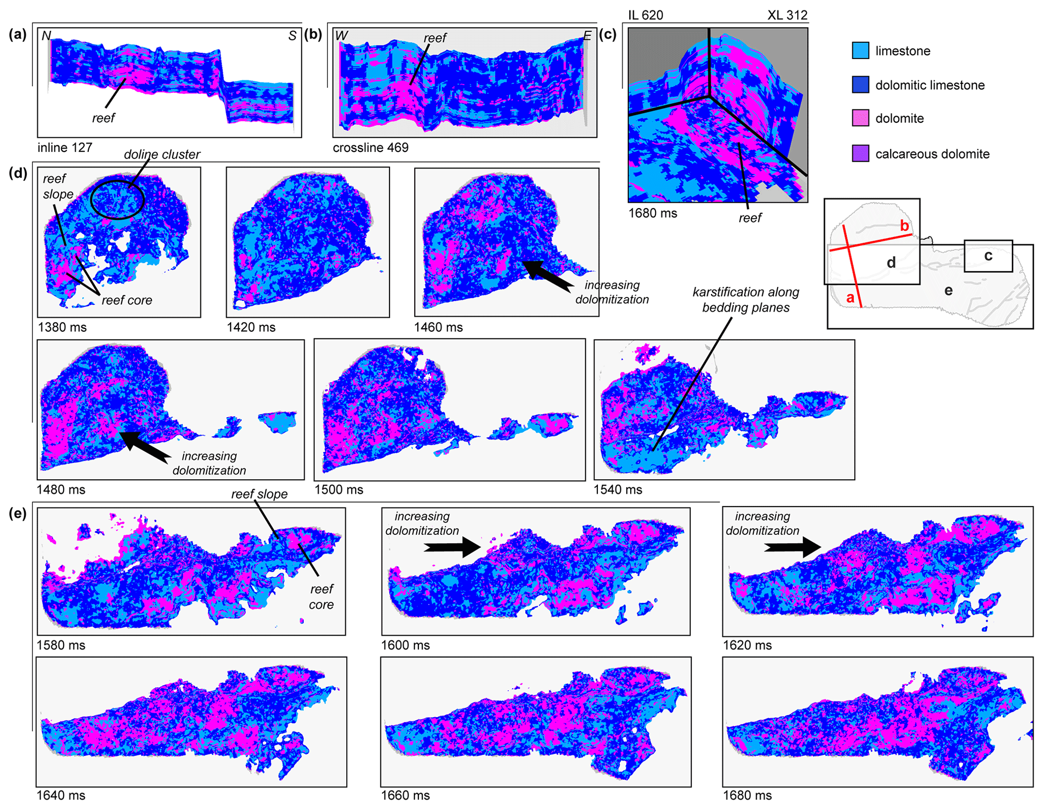
Figure 12Cross-sections and time slices through the 3D lithology model derived from the neural network classification of the seismic attributes. The model enables the interpretation of the vertical and lateral distribution of the different carbonate types and allows the identification of dolomitization trends at local scale within reefs (a–c) and at regional scale on the footwall (d) and on the hanging wall of the Munich Fault (e).
By investigating individual time slices in the top view (Fig. 12d and e), we noticed that areas can be defined in which certain lithology types are dominant. For the entire reservoir of the GRAME study site, the upper part is dominated by limestone and dolomitic limestone for both the footwall block (e.g. at 1380 ms) and the hanging-wall block (e.g. at 1540 and 1580 ms). Apart from that, it is noticeable that the footwall block shows higher degrees of dolomitization in the west and northwest compared to the east and southeast (e.g. at 1460 ms). On the other hand, the hanging wall shows the opposite trend with increased dolomitization to the east and in the central part (e.g. at 1600 and 1620 ms), although this spatial trend diminishes towards greater depths (e.g. at 1660 ms). Overall, dolomitization appears to be slightly more pronounced on the hanging-wall block than on the footwall block. Additionally, the subdivision of the reservoir into a lower part with almost completely dolomitized carbonates and an upper part with more partially dolomitized carbonates could indicate several dolomitization and dedolomitization phases.
With regard to the reefs, the time slices show the same lithology distribution as observed in the cross-sections, with mainly dolomite in the reef cores and dolomitic limestone and limestone at the reef slopes and in the upper parts of the reefs (e.g. at 1380 and 1580 ms). According to the results of Wadas and von Hartmann (2022), who showed that the reef slopes and the reef caps have higher porosities compared to the reef cores due to karstification, it is assumed that limestone and dolomitic limestone in the reefs appear to be more prone to karstification than the areas of pure dolomite. Similar observations can be made in areas comprised mostly of limestone-dominated carbonates and show intense karstification, e.g. the sinkhole cluster in the north of the footwall block (e.g. at 1380 ms) or the western part of the hanging wall (e.g. at 1540 ms) with karstification along bedding planes according to Wadas and von Hartmann (2022).
In addition, we could not find any other correlations between structural characteristics and the spatial distribution of dolomitization. For example, the amount of dolomite is not increased at faults or intensely fractured areas with increased permeability, such as in the east of the footwall block. This indicates that dolomitization in the Munich area is more facies-controlled than fault-controlled.
4.3 Comparison of FOA derived from well and seismic data
An important question that is often raised in reservoir exploration addresses the scalability of fracture properties like the orientation and size. To address this question, we compared fracture orientations (FOs) in the vicinity of the well paths derived from the seismic attribute analysis with the CMI results. Results are grouped in the following according to the tectonic blocks to facilitate comparisons within the three fault blocks of the Munich Fault.
On the footwall the fracture orientations (dip direction/dip angle) and derived fracture clusters for the wells show both good and poor agreement. Regarding Th3, only the seismic results are shown due to data restrictions of the corresponding image interpretations. Overall, the seismic data (Fig. 13) reveal three fracture clusters at 346/01, 290/01, and 233/01. However, we observe a change in the fracture systems with depth. In the depth range between 1730 and 1810 m, we observe two fracture clusters at 338/01 and 67/06. In the depth range between 1810 and 2050 m, we observe three fracture clusters; the main cluster (173/11) is comparable to the upper part, but we observe two new clusters at 72/09 and 310/26. In the deepest part between 2050 and 2190 m, we observe a broad range in fracture orientations and no distinct clusters can be identified. For well Th5, which was drilled mainly in dolomitic limestone, the fracture clusters show a variable match between the seismic and image analyses (Fig. 13). In general, the seismic data with four clusters show a more diverse distribution in fracture orientations than the CMI data with just two clusters. A good match with ±15∘ is accomplished for the 282/01 cluster (from seismic data) and the 284/03 cluster (from CMI data). A moderate match with ±30∘ is observed for the 159/05 fracture cluster (from seismic data) and the 176/06 cluster (from CMI data). Two other fracture orientation clusters that we observe in the seismic data are not present in the CMI data. To analyse whether the variable match holds for the complete well path or not, we also compare fracture orientations within different depth sections separately. We observe that in the upper depth range between 1680 and 2000 m that consist of bedded and massive facies, one of the two clusters shows a good match. A second cluster identified in the seismic is not observable in the well. In the lower part from 2000 to 2130 m, which is mostly of bedded facies, the fracture clusters show a poorer match, whereby in the seismic data the E–W-striking fracture set is split into two (conjugate) sets.
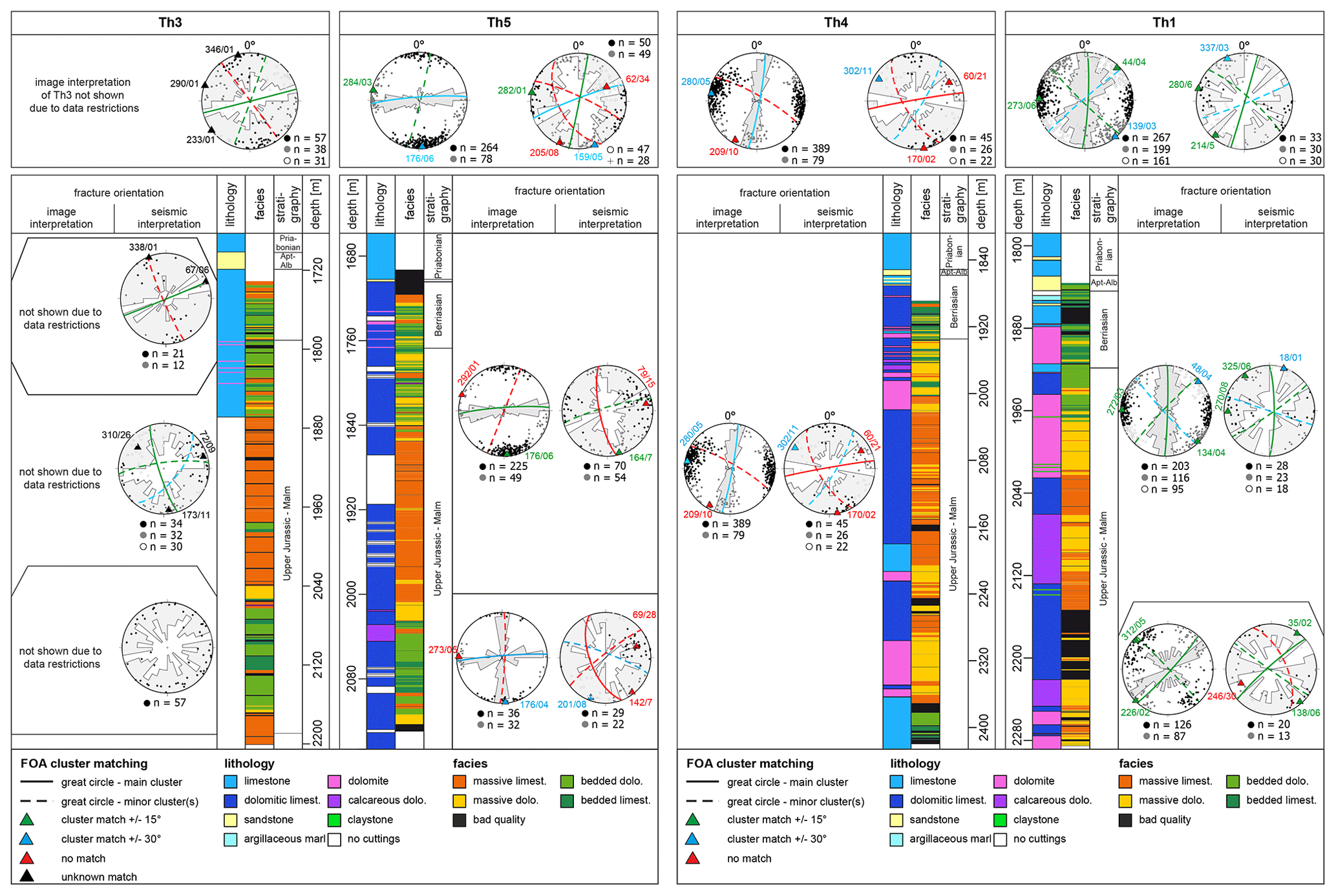
Figure 13Comparison of fracture orientations from seismic and CMI data from the wells on the footwall (Th3 and Th5) and the intermediate block (Th4 and Th1) of the Munich Fault using rose diagrams and stereographic pole plots. Seismic fracture orientations are shown by white rose diagrams, and CMI fracture orientations are shown by grey rose diagrams, together with colour-coded fracture cluster matching. For each well the lithologies, facies types, and stratigraphy are given.
On the intermediate block, a strong well-dependent distinction with respect to matching fracture clusters between seismic and CMI data is evident. For well Th4, which was drilled mostly in dolomitic limestone of the massive facies and to a minor degree of limestone and dolomite, a poor cluster match is found, with the closest match for one cluster within an angle of ±30∘ (Fig. 13). Notably, fracture orientations are stable along the entire well path. In contrast, Th1 (Fig. 13) in the east of the intermediate block, which was drilled in dolomite, dolomitic limestone, and calcareous dolomite, shows a good fit of fracture orientations, with two clusters fitting with ±15∘ (seismic data: 280/06 and 214/05; CMI data: 273/06 and 44/04) and one matching with ±30∘ (seismic data: 337/03; CMI data: 139/03). Similar to Th5, the quality of the cluster match between CMI and seismic data changes with depth; i.e. the fit between the clusters is better in the upper part of the reservoir (1840 to 2180 m) compared to the lower part (2180 to 2290 m). The upper part consists mostly of a bedded and a mixed facies, whereas the lower part consists of massive dolomite.
On the hanging-wall block (Th2a and Th6), when comparing fracture orientations over the entire well paths, we observe that the quality of the match between seismic and CMI data is better for well Th6. Th6 was drilled mostly in massive limestone and in the upper part to a minor extent in bedded limestone. In the seismic data we found three fracture clusters that show either a good (seismic: 240/04; CMI: 233/01) to moderate (seismic: 117/02; CMI: 137/01) fit with ±15 to ±30∘ or no fit (002/16) with the CMI data (Fig. 14). Furthermore, we observe variations of the fit with respect to depth. For example, the upper and lower parts of Th6 both have clusters that are a good match within ±15∘ and clusters that are a moderate match within ±30∘. In the middle part the fit is poor; i.e. only two clusters match within ±30∘. For the entire well Th2a (Fig. 14), drilled mostly in massive dolomite and massive dolomitic limestone, only a poor cluster fit is found. Only one fracture cluster fits within ±30∘ (seismic: 333/12; CMI: 001/04). Additionally, in the seismic as well as in the CMI data one fracture set exists that was not identified by the other method. The depth-dependent fracture fit shows that in the upper part between 2020 and 2400 m depth at least the rough orientation fits. In the lower part a reliable comparison is not possible because of the low number of measurements in the CMI data. However, both methods show a roughly NE–SW- and a NW–SE-striking fracture set.
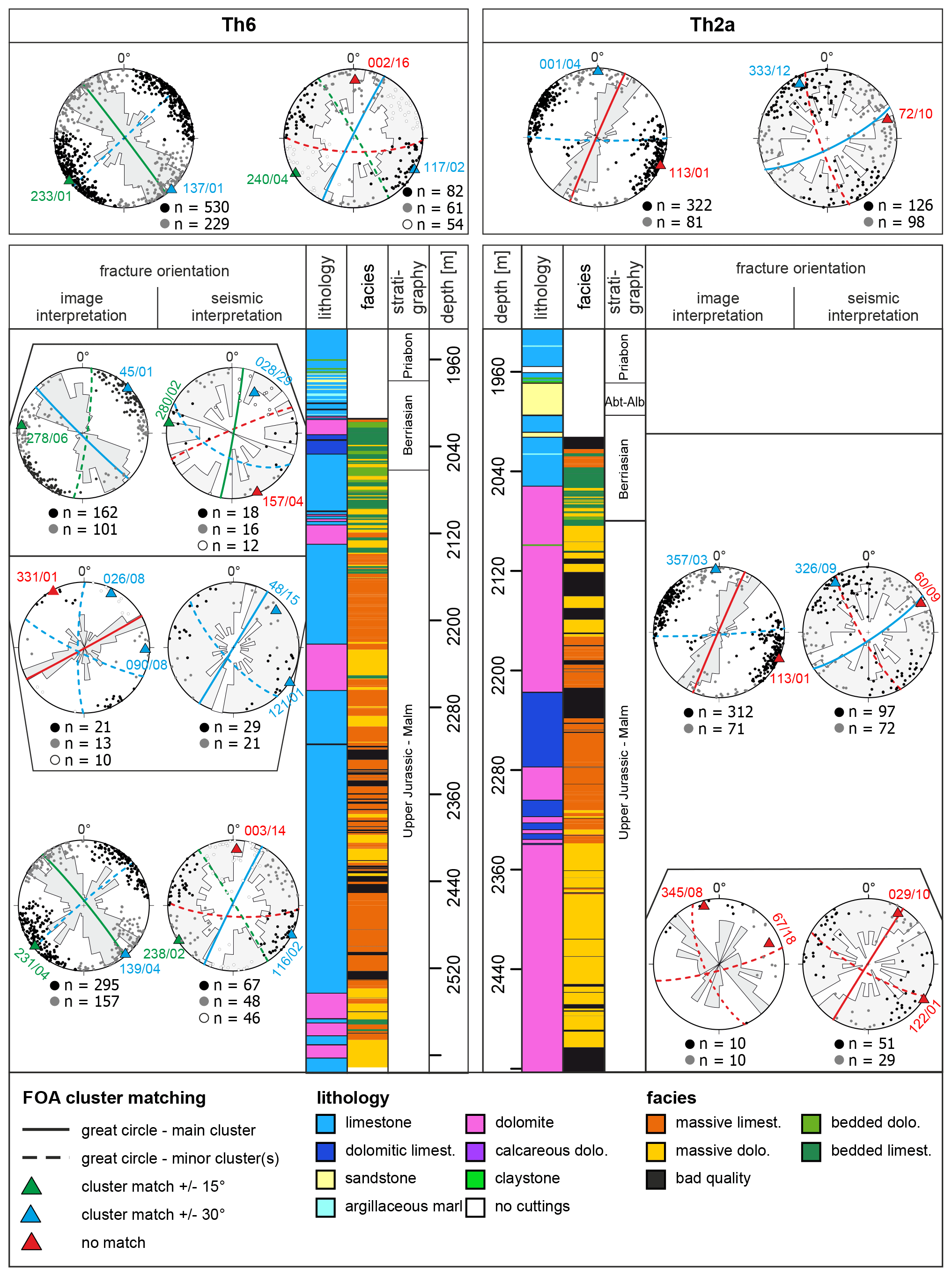
Figure 14Comparison of fracture orientations from seismic and CMI data for the wells on the hanging wall (Th2a and Th6) of the Munich Fault using rose diagrams and stereographic pole plots. Seismic fracture orientations are shown by white rose diagrams, and CMI fracture orientations are shown by grey rose diagrams, together with colour-coded fracture cluster matching. For each well, the lithologies, facies types, and stratigraphy are given.
In summary, correlations between lithology or facies and well location are evident with respect to the matching of fracture clusters. Fracture orientations in massive limestone show a better match than in massive dolomite. Independent of facies, the degree of dolomitization seems to correlate negatively with scalability. With regard to the well locations, differences can be detected within the fault blocks in terms of corresponding fracture orientations. On the footwall, Th3 in the west is located in mostly undisturbed material compared to Th5, which is situated in disturbed rocks according to the discontinuity attribute analysis. Furthermore, the area around Th5 also has slightly higher porosities than the area around Th3 according to the porosity model (Wadas and von Hartmann, 2022), indicating that the area around Th5 is more affected by fault- and probably karst-related deformation. This led to the generation of fractures with more diverse orientations, as observed for Th5. Therefore, Th5 shows a poorer match than other wells. Based on this assumption, we expect a much better FO match for Th3 because the well and its surrounding are situated in mostly undeformed material, and as a result, the preferred fracture orientations should also show up more clearly in the seismic data compared to Th5. On the intermediate block, Th4 shows almost no fitting fracture orientations compared to Th1, which is probably also a result of more intense fault-related deformation because Th4 is located at the branching point of the Munich Fault where it splits into two fault branches. On the hanging wall, Th6 in the west shows a slightly better FO match than Th2a, probably due to slightly enhanced fault-related fracturing more to the eastern part of the fault block. Overall, the seismic analysis is able to distinguish several fracture orientation sets or groups, similar to the CMI analysis, striking NNE–SSW, NE–SW, ENE–WSW, NW–SE, and NNW–SSE.
The benefit of seismic attributes is to highlight contrasts in the data. However, the more complex a reservoir is, the more difficult it is to interpret these contrasts. Due to their strong heterogeneity, the characterization of carbonate reservoirs is therefore a major challenge in exploration (e.g. Ehrenberg and Nadeau, 2005; Lucia, 2007). In the following, first the chosen methodical approach is inspected, and afterwards we discuss the scalability of fracture orientations as well as the structural and diagenetic evolution of the reservoir. Taking all results into account, we provide new exploitation targets in the Munich area for possible future geothermal projects.
5.1 Methodical approach
We have demonstrated the benefits and a number of applications of seismic attribute analysis for the characterization of a geothermal carbonate reservoir in the GMB. In the following, we discuss aspects regarding the calculation and the usage of seismic attributes that need to be considered.
Seismic attributes are a quantitative measure of the seismic data. They are sensitive to geology and thus allow drawing conclusions about the structural interpretation or characterization of the depositional environment, e.g. faults, stratigraphy, and geomorphology (Chopra and Marfurt, 2007). Since their first application in the 1970s, a large number of seismic attributes were developed, which makes it difficult to select the appropriate ones for a specific analysis (Chopra and Marfurt, 2007). According to Barnes (2006), the following criteria should be considered to avoid the use of unnecessary attributes: discard duplicate seismic attributes (if there are multiple attributes that measure the same property, choose the one that works best for your data) and prefer attributes with geological or geophysical meaning. To avoid duplicate attributes in our study, cross-plot analyses were performed not only between the attributes and the lithology logs, but also between the attributes themselves. In the case of a linear or quadratic relationship, which indicates that the attributes contain nearly the same information, one of the attributes was discarded from further analyses. Furthermore, all chosen attributes have geological and/or geophysical meaning linked to the reservoir characterization.
The effectiveness of seismic attribute analysis is also controlled by the type of reservoir. The great advantage of seismic attributes is to highlight contrasts in the data. However, the more complex a reservoir is, e.g. regarding control factors (reef development, karstification, and dolomitization), the more difficult it is to interpret these contrasts. Therefore, prior knowledge of possible reservoir control factors that might affect the physical rock characteristics, e.g. density, is important when performing the seismic attribute analysis itself. This is because the properties of a seismic wave, e.g. velocity, amplitude, frequency, phase, and attenuation, change while the wave propagates through the subsurface, and these changes are caused by the physical differences of the various rocks and geological structures (Taner, 2001; Chopra and Marfurt, 2007; Veeken, 2007). In addition, it should be kept in mind that the quality of a seismic attribute analysis can be negatively influenced, e.g. by acquisition footprints, processing artefacts, and noise (Marfurt and Alves, 2015). Therefore, a quality check of the seismic data prior to analysis is a necessity.
Almost all attribute analyses can be adapted to the object under investigation to obtain viable results by changing parameters such as the inline and crossline radii or the number of samples or traces (Chopra and Marfurt, 2007; Schlumberger, 2020). If the goal is e.g. the interpretation of large-scale faults, rather large spatial parameters should be chosen; e.g. in the variance analysis a lateral range of eight inlines and crosslines should be used. However, for the investigation of fractures, the analysis should be carried out on a smaller scale, which is why we chose a range of three inlines and crosslines in our study. The same holds for the identification of karst structures, such as dolines, that are characterized by small-scale lateral and vertical variations, which is why small investigation windows were chosen. The investigation scale also played an important role for the ant-tracking algorithm because the presented workflow can also be used for the identification of large-scale faults and the extraction of corresponding fault patches. The parameters should be adjusted accordingly, for example, by changing the ant-tracking mode from aggressive to passive and e.g. the initial ant boundary from a close distribution (two voxels) to a coarse distribution (six voxels). Therefore, it must be clear beforehand what is to be highlighted with the attribute analysis in order to select the appropriate parameters for the calculation.
Besides single-attribute analyses, the application of multiple seismic attributes in a combined plot is a key element of our study. They are generally usable in various clustering techniques, like self-organized maps (Roden et al., 2015; Zhao et al., 2015), geostatistics (Janson and Madriz, 2012; Ba et al., 2019), and neural networks (Brcković et al., 2017; Gogoi and Chatterjee, 2019; Abdel-Fattah et al., 2020), that have gained a lot of attention in recent years because they enable parameter-based classifications, e.g. to obtain a 3D lithology or facies reservoir model. The quality of the results strongly depends on the input data such as seismic attributes and, in the case of availability, the desired output data (e.g. lithology logs from wells). With regard to the input data, it is important to note that these must show a correlation between the physical parameters derived from the seismic attributes and the desired classes. A correlation coefficient close to 1 indicates a perfect or almost perfect match between the datasets. However, this is usually not the case for geological correlations because rocks are generally heterogeneous, e.g. with regard to their petrophysical parameters or their composition. A correlation coefficient close to zero indicates that there is no relationship between the different datasets, which would make it impossible to achieve a good mathematical model that can be used for lithology prediction. Thus, only attributes with acceptable correlations should be implemented in the classification because incorporation of attributes with low or no correlations would degrade the quality of the classification (Zhao et al., 2015). Therefore, we decided to choose only a small number of attributes that enable an acceptable classification. However, it should be kept in mind that the classification carried out in this study is based solely on different types of carbonates, which show minor physical differences. High correlation coefficients are therefore not to be expected. Besides the correlation analysis, we were also able to use a supervised neural network for the lithology classification, since six wells with corresponding lithology logs were available, which were used as the desired output data. Due to the fact that no large variations of the physical parameters between the different carbonate types were to be expected, a manual classification or an automatic classification with an unsupervised neural network that only looks for data trends would have hardly yielded promising classification results with a geological meaning. When using logs as boundary parameters, however, it should be noted that these should cover the entire range of the classes and therefore the heterogeneity of the reservoir in order to enable a reliable assignment. As a consequence, the more heterogeneous the reservoir, the more wells should be implemented into the classification. With regard to our study, the implementation of only one or two wells might not be sufficient to obtain a representative lithology classification of the heterogeneously distributed carbonate types; e.g. Th5 contains mostly dolomitic limestone, Th2a contains mostly dolomite, and Th6 contains mostly limestone. Therefore, implementation of all six lithology logs delivered a more comprehensive overview of the different carbonate lithology types within the reservoir. Nevertheless, it is important to keep in mind that only a small part of the reservoir is covered by the six wells, which will always lead to a certain degree of uncertainty.
With respect to the identified classes, we chose to differentiate between the four carbonate types limestone, dolomitic limestone, dolomite, and calcareous dolomite, although the latter appears only sporadically. We chose this classification because other studies have shown that, for example, dolomitization can have a major influence on reservoir quality, especially on porosity and permeability (Reinhold, 1998; Koch et al., 2010; Böhm, 2012; Mraz, 2019; Bohnsack et al., 2020). There are other classification options, but a classification, e.g. according to the two hyper-facies types (massive and bedded facies), would not have made geological sense, as many studies have shown that the presence of massive facies alone is no guarantee of good reservoir conditions. For example, massive facies can also have poor porosity and/or permeability conditions due to e.g. cementation, compaction, and overdolomitization (Schmoker and Halley, 1982; Lucia, 2007; Wolfgramm et al., 2011; Homuth, 2014), whereas bedded facies can also be suitable for exploitation e.g. due to karstification along bedding planes and thus increased porosity and/or permeability values (Lucia, 2007; Mraz, 2019; Wadas and von Hartmann, 2022). A further facies differentiation incorporating the lithology types and also the fabric types (e.g. laminated, banded, ordered or unordered clasts, clast size) would be necessary, but since the different facies classes did not show clear correlations with the seismic attributes because the rock-physics-based parameters did not vary strongly enough due to too many subdivisions, a reliable classification was not possible. Therefore, we limited the classification to the lithology types.
It should also be noted that we used only volume attributes in this study but no horizon attributes because surface or horizon attributes require the horizons or surfaces to be accurately picked. Regarding the Jurassic carbonates, this would only be possible for the top of the reservoir. Internally, however, no horizons or surfaces could be picked due to the complex structural conditions (e.g. the presence of faults, fractures, and dolines) and the complex lithology and facies distribution (e.g. bedded and massive facies). Seismic pre-stack attributes based on amplitude versus offset (AVO) analyses, for example, were also not investigated, since an AVO analysis had not been carried out for the GRAME dataset at the time of this study and only the finished stacked datasets were available. AVO attributes enable the offset-dependent investigation of physically relevant parameters of the reservoir and have provided promising results in other reservoir studies (Veeken, 2007; Barclay et al., 2008; Bredesen et al., 2020). For this reason, we recommend that AVO analyses be carried out together with the classical post-stack attribute analysis in the exploration phase of future geothermal projects.
5.2 Scalability of fracture orientations
The comparison of fracture analyses from seismic and CMI data allows drawing conclusions regarding the scalability of fractures in the GRAME area. As shown, the fracture orientations fit only under certain circumstances; thus, a general scalability across the two scales, namely seismic and well scales, is not given.
Possible reasons that fractures cannot be scaled between seismic and drilling scales may be of geological but also of methodological origin. Regarding the geological reasons, von Hartmann et al. (2012), Lüschen et al. (2014), and Ziesch (2019) have proven the existence of fault-related deformation for the Munich region, which according to our study seems to influence scalability. Areas that are more affected by tectonic stress show poorer scalability than areas with less deformation; e.g. the fault damage zones in the intermediate block and between the Munich Fault and the Nymphenburg Fault lead to more intense fracturing, not only on the seismic scale but also on the sub-seismic scale (Lohr, 2008; Ziesch, 2016; Ashton et al., 2018). Therefore, not all fractures in these areas are detectable by the seismic survey, especially if the fractures on the sub-seismic scale have a different orientation than those on the seismic scale, resulting in non-matching fracture clusters. Another control factor is karst-related deformation. Dissolution of rocks can lead to cavities, and over time new, especially small-scale, fractures can form in the surrounding areas due to collapse and local stress redistribution (e.g. Parise and Lollino, 2011; Salmi et al., 2017; Al-Halbouni et al., 2018; Shiau and Hassan, 2021). These fracture orientations do not have to follow the local stress field, but can spread e.g. radially away from the cavity (Schneider-Löbens et al., 2015; Rawal et al., 2016; Al-Halbouni et al., 2018). Thus, differences in the identified fracture orientations and fracture scalability can arise because these locally restricted fractures may not be detected on the seismic scale, but they can be captured on the CMI scale. However, the results of this study indicate that dolomitization is another factor that influences scalability; e.g. scalability decreases with increasing degree of dolomitization. During dolomitization, recrystallization leads to a reduction in rock volume, which can cause further fracturing, and for that reason, dolomite tends to have a higher fracture intensity compared to limestone (Korneva et al., 2018; Liu et al., 2020). To further validate these assumptions, additional analyses at other study sites are necessary. In summary, fracture scalability is possible but highly depends on the complexity of the geological conditions on the sub-seismic scale.
Regarding the methodological reasons for different fracture orientations in seismic and CMI data, the different resolution limits of the two methods have already been mentioned. However, another important point is that a CMI analysis only covers a very small volume, whereas 3D seismic attribute analysis allows a more comprehensive spatial analysis (Fang et al., 2017; Albesher et al., 2020; Boersma et al., 2020; Loza Espejel et al., 2020), and this may result in the detection of differing fracture orientations. In nature, fractures can change their orientation along the fracture path. Therefore, dip directions and dip angles can vary depending on where along the fracture path the orientation is measured. As a result, the values of the fracture orientations from the seismic data always represent an average value over the entire fracture path and not only a small part of the fracture path, as is the case with the CMI data, although the CMI delivers a more accurate result for a specific investigation point. Therefore, the CMI may be less accurate in detecting large-scale structures than the 3D seismic, so the abundance distribution or intensity (n value) of the preferred fracture orientations may be different based on the chosen method since different fracture sets may be captured. Furthermore, it also has to be considered that the n value in the CMI and the seismic data can vary considerably because e.g. several parallel to sub-parallel fractures visible in the CMI data are imaged individually, whereas the seismic data may only image them as a single fracture (with an averaged orientation) due to the seismic resolution. This means that a comparison of the n values between seismic and CMI is not very meaningful. In addition, the different imaging of fracture orientations in the CMI data compared to the seismic data could be influenced by the well orientation, which introduces an orientational bias; e.g. fractures (sub)parallel to the well can become underrepresented. With regard to the reflection seismic data, there are also methodical pitfalls that should be kept in mind. For example, not every discontinuity detected by the seismic attributes has to be a real fracture, since it could be e.g. an imaging artefact. Even if it is a real fracture, the derived geometric properties might be incorrect due to a wrong analysis window for the attribute calculation. For example, according to Marfurt and Alves (2015), coherence anomalies become increasingly more vertical the larger the analysis window is, resulting in a stairstep structure. Therefore, when analysing small features like fractures, small analysis windows must be chosen, as we have tried to do (see also the details on the chosen attribute parameters in the Appendix). Nevertheless, a small percentage of uncertainty in the derived fracture geometries, which cannot directly be quantified, must be expected. Another problem is possible lateral velocity variation of the seismic wave, inducing velocity pull-ups and push-downs that can cause false structures in the seismic image. For example, high-velocity anomalies result in a velocity pull-up and can generate subvertical “fractures” (Marfurt and Alves, 2015). Furthermore, it must be considered that not all fractures, which are theoretically present in the seismic raw data, are captured by the attribute analysis. Processing steps, especially filters or smoothing algorithms that are often used to enhance horizons, might remove real fracture information from the data unintentionally instead of preserving or highlighting them when processing parameters are chosen incorrectly. Another reason for the possible capture of too few fractures is scattering of the seismic wave at objects that are smaller than the wavelength. The resulting energy dispersion can then lead to fracture zones appearing as shadow zones in the seismic image and thus the fractures are not directly visible (e.g. Beilecke et al., 2016).
Overall, we conclude that both methods have their advantages and disadvantages. In our results we show that even with such a high data density in a comparatively small volume both methods produce results that are not generally comparable. However, we recommend using both fracture orientation analysis methods. The seismic-based FOA is a useful addition to the CMI-based FOA, as it allows fracture orientations to be investigated at different scales, and the combination of the two analyses provides a more complete picture of the fracture inventory and local fracture orientation trends. This can also be helpful when implementing fractures in other analysis methods such as hydraulic–mechanical modelling (Dussel et al., 2016; Bauer et al., 2019; Konrad et al., 2019). The seismic-based FOA can also be used to improve the planning of well paths. However, the seismic analysis cannot replace a later detailed CMI analysis, especially in areas with such complex geological conditions as the Munich region.
5.3 Diagenetic and structural evolution of the reservoir below Munich
With the increasing economic use of the subsurface in the GMB, especially in the context of geothermal exploitation and the associated scientific exploration, more has become known about the geological development of the region. A better understanding of the geological evolution of the GMB, especially of the geothermal reservoir, is of great importance in order to identify controlling factors and to better estimate the exploitation potential. As already mentioned, the most important reservoir control factors in our study area are (I) the lithology and thus the diagenetic evolution of the carbonates, (II) the distribution of massive and bedded facies, (III) the tectonic evolution and the influence of faults and fault-related fractures, e.g. on fluid pathways, and (IV) the karstification processes that can also improve permeability through the formation of cavities and additional fractures due to stress redistribution. So far, these control factors have been determined primarily by well log analyses. 3D seismic data are not always available, and even when such data have been measured, they have primarily been used for structural geological interpretations in the past. However, 3D seismic data, particularly seismic attributes, also allow spatial interpretation of lithology, diagenesis, and karstification as shown in this study. Therefore, in the following, existing concepts for reservoir development from spatially constrained drilling studies in the GMB, e.g. cutting analyses and formation micro-imager (FMI) log analyses (Reinhold, 1998; Koch et al., 2010; Koch, 2011; Wolfgramm et al., 2011; Böhm, 2012; Beichel et al., 2014; Mraz, 2019; Bohnsack et al., 2020), are discussed, and an extended conceptual reservoir model for the Munich area is presented that also incorporates spatial variations based on the 3D seismic analyses carried out in this study.
A recent reservoir concept of the Upper Jurassic carbonates in the GMB, presented by Mraz (2019) and based on older works e.g. by Reinhold (1998), separates the diagenetic evolution of the Upper Jurassic carbonates into five phases: sedimentation, early diagenesis and first dolomitization, burial diagenesis and second dolomitization, late burial diagenesis, and the present-day reservoir. Taking into account the spatial analyses based on the seismic results of this study, it is concluded that, in addition to the different dolomitization phases, there were at least two karstification phases and also various events that significantly influenced the fluid pathways, whereby these processes also partially influenced or triggered each other. We have therefore expanded the reservoir development concept accordingly. Our extended reservoir development concept comprises the following steps: (1) sedimentation and reef development, (2) early diagenesis and first dolomitization, (3) burial diagenesis and second dolomitization, (4) subaerial exposure and widespread karstification and erosion, (5) Alpine Orogeny and fault development, (6) late burial diagenesis and third dolomitization, (7) intense karstification along faults, and (8) continued subsidence (Fig. 15).
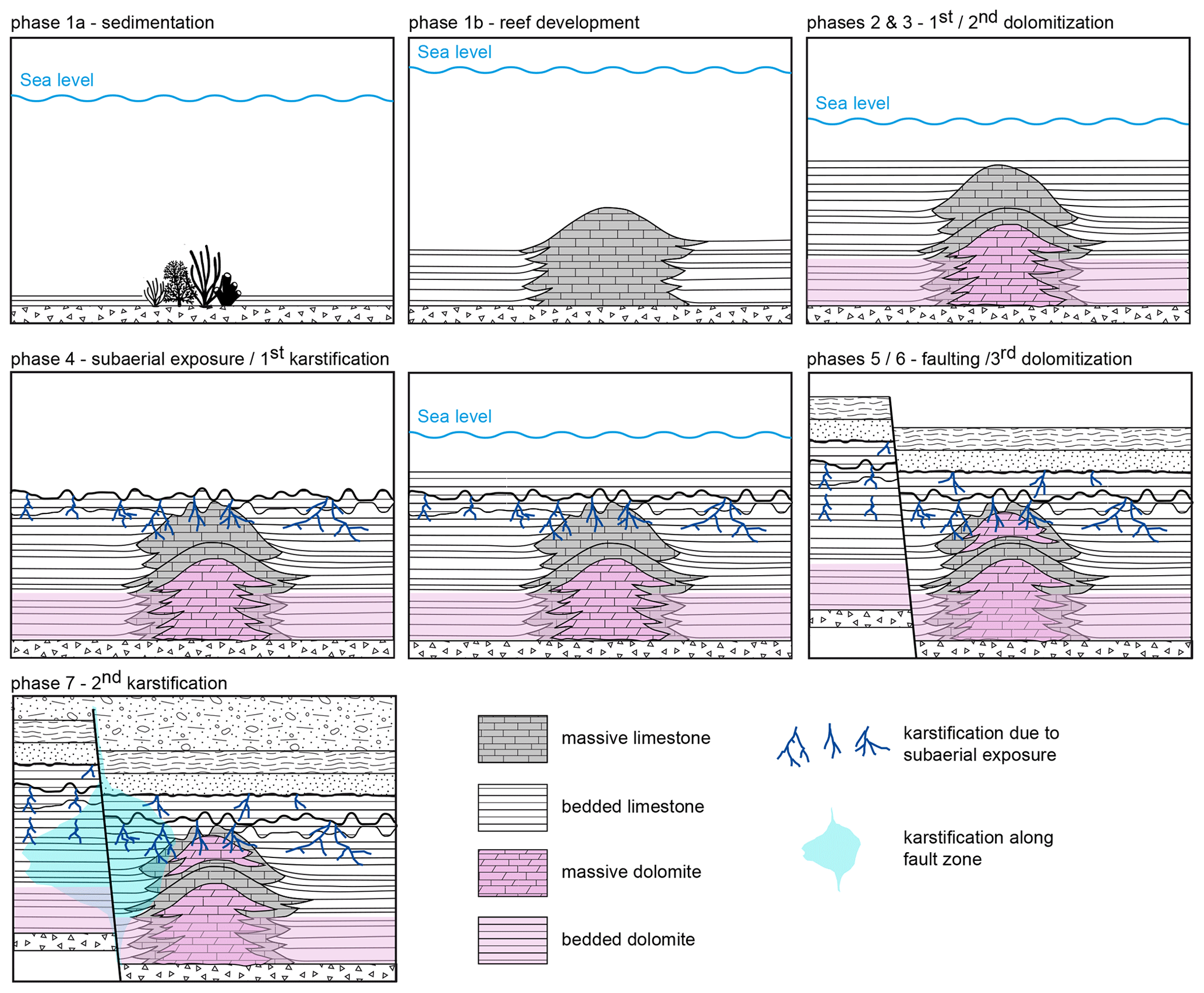
Figure 15Schematic illustration of the reservoir development concept with its different phases: (1) sedimentation and reef development, (2) early diagenesis and first dolomitization, (3) burial diagenesis and second dolomitization, (4) subaerial exposure and widespread karstification and erosion, (5) alpine orogenesis and fault development, (6) late burial diagenesis and third dolomitization, (7) intense karstification along faults, (8) and further subsidence. Phases 8 is not shown.
(1) Sedimentation and reef development. During the Upper Jurassic high amounts of carbonate were deposited in the study area that was covered by the Tethys Sea at that time (Schmid et al., 2005; Pieńkowski, 2008), which was also accompanied by the development of the reef buildups found in the GRAME area. As shown by the high-resolution acoustic impedance model derived from the GRAME 3D seismic data by Wadas and von Hartmann (2022), the massive facies of the reef slopes inter-finger with the surrounding bedded facies, forming rounded “pine-tree”-shaped edges. This was interpreted as an indication of syn-sedimentary reef development with varying growth rates. The reef geometry also seems to narrow towards the top, especially in the upper third of the reef. This narrowing is postulated to result from long-term sea level changes during the Upper Jurassic. According to Haq (2017), the sea level in the Oxfordian (Malm α to Malm β) and Kimmerdigian (Malm γ to Malm ϵ) rose from approximately +50 to approximately +150 m (compared to today's sea level), and it dropped again to about +100 m by the end of the Tithonian (Malm ζ). Since our study area was located in a shallow-marine environment at that time, we assume that these sea level fluctuations had a significant influence on the carbonate production rates and thus also on the reef structure in the Munich area. A sea level rise often enhances carbonate production, while a sea level fall can hamper carbonate production and therefore reef growth, especially in combination with enhanced erosion at the shallow coastline (Kendall and Schlager, 1981; Pomar and Ward, 1995). This is confirmed by the observation that the upper part of the reef buildups, mainly consisting of Malm ζ, shows a decrease in lateral reef growth. Furthermore, the observed varying pine-tree-shaped reef slopes (Wadas and von Hartmann, 2022) might correlate with short-term sea level changes. The fact that sea level fluctuations have had an impact on our study area is important because they can also influence diagenetic processes, especially in shallow-marine environments; e.g. at low sea levels, freshwater diagenesis dominates, whereas at high sea level, seawater diagenesis dominates, and if the area is completely exposed, erosion and karstification may also occur (Kendall and Schlager, 1981; Tucker and Wright, 1990; Bachmann and Müller, 1992). With regard to the further reservoir development, it is therefore important to know that, in general, the sea level fell further at the beginning of the Early Cretaceous down to +50 m and then rose again during the Cretaceous to up to +250 m, only to fall again in the Tertiary and Quaternary until it reached the present sea level (Haq, 2017).
(2) Early diagenesis and first dolomitization as well as (3) burial diagenesis and second dolomitization. The early burial diagenesis directly after deposition of the carbonates caused the first dolomitization phase and therefore the formation of matrix dolomite due to the contact with Mg-rich basinal fluids at 50 to 70 ∘C (Mraz, 2019). This was directly followed by the second dolomitization phase during burial diagenesis. According to several studies which investigated deep wells in the GMB and outcrops in the Franconian and Swabian Alb, the second dolomitization phase occurred at temperatures between 70 and 100 ∘C and involved an enormous fluid flow, e.g. through highly permeable limestone (Lucia, 2007), with high amounts of Mg-rich fluid, causing intense dolomitization (Reinhold, 1998; Machel, 2004; Mraz, 2019). The fluids might have originated from seawater stored within the carbonate formations, which migrated through the permeable formations of the massive and bedded facies during burial diagenesis, e.g. due to compaction-driven fluid flow (Reinhold, 1998; Machel, 2004). Our 3D lithology model (Fig. 12) shows clear spatial trends in the degree of dolomitization that can be assigned to the first two dolomitization phases and the later third dolomitization phase. Overall, the Upper Jurassic carbonates in the lower part of the reservoir are more completely dolomitized than in the upper part, especially on the hanging-wall block to the south, creating a lithological subdivision (Fig. 12). Furthermore, the footwall block shows a west–east to northwest–southeast trend, with higher degrees of dolomitization in the west, and on the hanging wall a rough trend with more intense dolomitization in the central part and the east can be seen. The intense dolomitization in the lower half probably results from the compaction-driven fluid flow of stored Mg-rich seawater during burial diagenesis. The reason for the slightly stronger complete dolomitization in the south of the study area could be that the former coastline of the Tethys was located to the north, and therefore the compaction pressure towards the south, induced by sediment and water load, would have been slightly higher, which may have enhanced mobilization of Mg-rich fluids. On the other hand, the west–east dolomitization trend on the footwall block and the east–west trend on the hanging-wall block seem to be more facies-controlled. According to several studies, e.g. by Reinhold (1998) and Mraz (2019), massive facies (reefs) is more prone to dolomitization than bedded facies. As a result, completely dolomitized areas partly correlate with reef buildups. Reefs are often characterized by grain-supported carbonates with biogenic components which are mostly highly permeable (Flügel, 2010; Böhm, 2012; Homuth et al., 2015), at least during and shortly after deposition and burial, enabling good conditions for enhanced fluid flow. This resulted in strongly dolomitized areas at the reef base and within the reef cores, especially in the lower half of the reservoir.
(4) Subaerial exposure and widespread karstification and erosion. The falling sea level during the Tithonian and especially at the Jurassic–Cretaceous boundary led to subaerial exposure of the study site due to a regression of the Tethys. This enabled widespread dissolution of the near-surface carbonate formations due to the contact with meteoric water (Bachmann et al., 1987; Bachmann and Müller, 1992; Reinhold, 1998; Koch, 2011), which created a strong karst topography with many small-scale dolines or sags, visible as blue-coloured dots in the shape index attribute (Fig. 11), covering the entire carbonate surface. Dissolution and the associated karstification led to the formation of secondary porosity, an enlargement of the already existing pore space, and the formation of cavities. Furthermore, later cavity collapse can result in the formation of new fractures due to local stress redistribution in the surrounding material, which is visible in the seismic attribute analysis by a strong scattering of the seismic waves at the doline edges, e.g. shown by low frequencies (Fig. 6) and high variance values (Fig. 9). Thus, karstification can improve both the porosity and the permeability conditions of a reservoir. However, should the fluid solution become supersaturated at some point or in the case of pressure and temperature changes, precipitation and thus cementation can occur, which in turn can have a negative effect on porosity and permeability. The same applies for dedolomitization, which is often triggered due to contact with Ca-rich meteoric water; this enables the transformation of dolomite back into limestone (Raines and Dewers, 1997; Reinhold, 1998; Koch, 2011), which in turn is usually accompanied by a deterioration in porosity and/or permeability conditions. Since only the upper part of the reservoir was affected by Ca-rich meteoric fluids over a long time, no dedolomitization is expected to have happened in the deeper parts of the reservoir (Mraz, 2019). However, since it is not possible to distinguish between partially dolomitized limestone and partially dedolomitized dolomite in the reflection seismic images, because it is expected that the physical properties of both types would be the same, possible dedolomitization is therefore not further discussed. Besides the karstification, another indication for the subaerial exposure at the Jurassic–Cretaceous boundary is the northeast–southwest-oriented channel cut into the carbonate deposits, which can be seen in the acoustic impedance (Fig. 4) and the spectral decomposition (Fig. 7). All these processes ended with the rise of the sea level during the Cretaceous, which again led to a flooding of the study area.
(5) Alpine Orogeny and fault development. The beginning of the Alpine Orogeny at the Cretaceous–Tertiary boundary led to extensive compressional deformation and therefore to the uplift of southern Germany (Lemcke, 1988). The tectonic deformation also led to faulting and the formation of fault-controlled fracture networks, which serve as fluid pathways for hydrothermal water, even in recent times (Mraz et al., 2018; Moeck et al., 2020). We analysed these fracture networks and their orientations in detail in the reflection seismic data and compared the seismic results with CMI results from the six wells at the Schäftlarnstraße geothermal site. The results reveal W–E-striking fractures parallel to the Alpine front, N–S-striking fractures perpendicular to the Alpine front and therefore parallel to SHmax, and NW–SE and NE–SW-striking conjugate shear fractures. However, the fracture orientations, especially in the seismic data, show a wide range of orientations, and it can be assumed that non-tectonic fractures, such as those caused by karstification and the collapse of cavities, also play a role in the fluid pathways and thus the permeability of the reservoir.
(6) Late burial diagenesis and third dolomitization as well as (7) intense karstification along faults. The fault and fracture-controlled fluid flow also influenced the further development of the reservoir, enabling a third dolomitization phase during late burial diagenesis and a second karstification phase. Diagenesis continued especially in the Eocene and Miocene, when fault-controlled dolomitization occurred due to seawater migrating downward along the faults into convection cells (density-driven circulation of fluids) where it was heated up, and the Mg-rich hydrothermal water then migrated back upward along the fracture networks, enabling dolomitization in the younger carbonate formations (Benjakul et al., 2020). The upper part of the reservoir contains mostly only partly dolomitized limestones, so we assume that either the fluid flow rates or the magnesium contents of the fluids were significantly lower than during the second dolomitization phase or even both together, which is why the dolomitization in the upper part of the reservoir area is less pronounced than in the lower part. Fluid migration of unsaturated water along the fractured fault zones was also the trigger for the second karstification phase. However, the dissolution processes and thus the karstification were concentrated along the fault zones and their immediate surroundings. As a result of the higher fluid flow rates and the resulting intensified dissolution, significantly larger and deeper, and this time fault-related, dolines were formed, e.g. along the Munich Fault and the Ottobrunn Fault. Both the third dolomitization phase and the second karstification phase thus altered the porosity permeability ratios of the reservoir again, creating more secondary pore space, especially in the upper part of the reservoir area, namely Malm ζ.
(8) Further subsidence. The underthrusting of the European plate below the Adriatic–African plate in the Late Eocene caused the Alpine nappes to extend northwards, which led to subsidence-induced development of the GMB (Frisch, 1979; Bachmann et al., 1987; Bachmann and Müller, 1992) and the formation of further faults, e.g. flexure-induced normal faults (Lemcke, 1988; Bachmann and Müller, 1992; Shipilin et al., 2020).
Overall, the Upper Jurassic carbonate reservoir experienced a complex evolution, consisting of at least three dolomitization phases, two karstification phases, and a phase dominated by tectonic deformation. We show that dolomitization in the GRAME area is mainly facies-controlled and that karstification is both facies- and fault-controlled. Karstification and cavity collapse generally lead to improved porosity and permeability conditions for hydrothermal exploitation, while dolomitization can lead to both an increase in secondary porosity and also a possible porosity decrease due to overdolomitization.
5.4 Exploitation targets
Based on the comprehensive 3D seismic characterization of the Upper Jurassic carbonate reservoir, two regions are identified that are likely to have suitable porosity and permeability conditions for future geothermal projects in the greater Munich area. The regions were selected according to the following criteria that are indicative of the important parameters permeability and porosity: lithology type, degree of dolomitization, facies type, karstification intensity, and fracture intensity.
The first recommended region is located in the southeast, at the Ottobrunn Fault. High porosities are expected here, according to the seismic inversion results by Wadas and von Hartmann (2022), due to partly dolomitized limestones and karstification along the fault zones. Furthermore, the area also contains some reefs with good permeability conditions because of high fracture intensities caused by mainly fault-related deformation, but also mass redistribution at the reef slopes, and due to cavity collapse and doline formation. The second region is located north of the Munich Fault in the vicinity of the Nymphenburg Fault. High porosities are caused by partly dolomitized limestone and widespread karstification. In contrast to the first region, this area is located in mostly bedded facies, and the karstification does not seem to be fault-controlled because no significantly large dolines are observed along the Nymphenburg Fault. Instead, mainly widespread karstification with large clusters of very small-scale dolines are observed. The widespread karstification and the influence of the fault zone also resulted in the generation of a presumably highly permeable reservoir.
With our case study from the South German Molasse Basin, we show that a comprehensive seismic attribute analysis can significantly improve the understanding of complex carbonate reservoirs. We address the following points: the physical and structural characterization of the reservoir, the question of the scalability of fracture orientations on seismic and well scale, the creation of a 3D lithology model, the temporal development of the reservoir, and the identification of further suitable exploitation targets in the GRAME area.
For the carbonates in the Munich area, we conclude that acoustic impedance is suitable to identify reefs, and sweetness has proven to be a useful tool to analyse the internal reef architecture, whereas frequency- and phase-related attributes are well suited for the detection of karst. In addition, reef edges, dolines, and fractures are characterized by strong phase changes. Fractures can also be identified using e.g. variance and ant tracking. Morphological characteristics, like bowl-shaped dolines, are captured using the shape index (see also Appendix Table B1).
Regarding fracture scalability across seismic and well scales, we state that a general scalability is not possible, although the fracture orientations are partially in good agreement. Limiting factors are methodological differences between seismic-based FOA and CMI-based FOA, as well as complex structural and lithological conditions, such as fault- and karst-related deformation on the sub-seismic scale and the degree of dolomitization. Nonetheless, we argue that seismic-based FOA can be a useful addition to the CMI-based FOA, since it allows investigating the fracture systems at different scales, and the combination of the two analyses provides a more complete picture of the fracture inventory and local fracture orientation trends.
With our 3D lithology model, based on a neural network, we investigated the reservoir development and exploitation targets. In terms of lithology, the dolomitized limestone should be targeted because of increased secondary porosity. Therefore, only reservoir zones should be exploited which have not been affected by strong diagenetic alteration. This concerns mainly the upper half of the Upper Jurassic carbonates with the Tithonian deposits. With regard to karstification, we conclude that it can lead to good porosity and permeability conditions for geothermal exploitation. As preferred karstification areas, we identify the upper part of the reservoir due to a previous subaerial exposure at the Jurassic–Cretaceous boundary and a later intensive karstification along faults related to the fault evolution during the Alpine Orogeny and the development of the foreland basin. Taking all the results into account, we identified two more locations in the Munich area that are likely to have preferable conditions for future geothermal exploitation projects: the region in the southeast at the Ottobrunn Fault and the region north of the Munich Fault in the vicinity of the Nymphenburg Fault.
Based on the promising results of our study, we recommend that in future geothermal projects much more comprehensive seismic analysis should be carried out. This comprehensive seismic analysis includes methods such as attribute analysis, inversion methods to calculate an impedance model in order to estimate a 3D porosity model, lithology and facies classification, and seismic fracture orientation analysis. The knowledge gained can help to develop a better understanding of the reservoir, its evolution, and the distribution of relevant exploitation parameters. Furthermore, the obtained data can also serve as input parameters for further studies, such as dynamic modelling, which strongly depend on the defined constraints. For example, when modelling stress changes in the uppermost crust during the theoretical operation of a geothermal doublet, it is important to have a comprehensive understanding of the fracture inventory. Information on fracture densities and fracture orientations, but also the spatial distribution of certain lithology and facies types, as well as karstification zones is also important in the context of thermal–hydraulic modelling.
Amplitude-related attributes
Three often used amplitude-related attributes are the root mean square (rms) amplitude, the reflection intensity, and the envelope. The rms amplitude is described as the square root of the sum of squared amplitudes divided by the number of samples within a specified time window (Chopra and Marfurt, 2007). The default window length in Petrel is nine samples (Schlumberger, 2020), but since we expected very small-scale variations of the energy content of the seismic data, e.g. at dolines and reef buildups, a window length of five samples was chosen after testing different windows. Another amplitude-related attribute that can help to distinguish different lithologies, and which was tested in this study, is the reflection intensity (Chopra and Marfurt, 2007; Sarhan, 2017), which is the average amplitude over a specified time window (five samples) multiplied by the sample interval. The envelope, also known as the instantaneous amplitude, is the magnitude of the complex trace described by envelope = , where f and g are the real and imaginary components of the seismic trace. It is independent of the phase and can therefore highlight lithological changes, sequence boundaries, and thin-bed tuning effects (Chopra and Marfurt, 2007). The default window length in Petrel is 33 samples (Schlumberger, 2020), but we chose 15 samples in order to depict small-scale variations.
As shown in the Appendix in Fig. A1, these three attributes can highlight areas with a much higher energy content compared to their surroundings, as can be seen e.g. in the western part of the footwall block (Fig. A1a, d, and g) of the Munich Fault and the eastern part of the intermediate block (Fig. A1b, c, e, f, h, and i). Such a strong difference in the amplitude, intensity, or envelope values can be an indicator for lithological, diagenetic, and/or depositional changes that affect the rock properties. Therefore, the larger but locally restricted high-amplitude anomalies on the footwall and the intermediate block are presumed to result from reef buildups. Such high amplitude values for reefs are also observed by other studies, e.g. Sarhan (2017). However, it has to be noted that since rms amplitude, reflection intensity, and envelope mainly identify strong anomalies, they are unsuitable to depict small variations in energy content, e.g. caused by karst-related dolines, especially on a small area, as it is the case in our study area. In general, this can hamper a sophisticated identification of structures or features and a detailed interpretation e.g. of the internal architecture of the reservoir features.
.
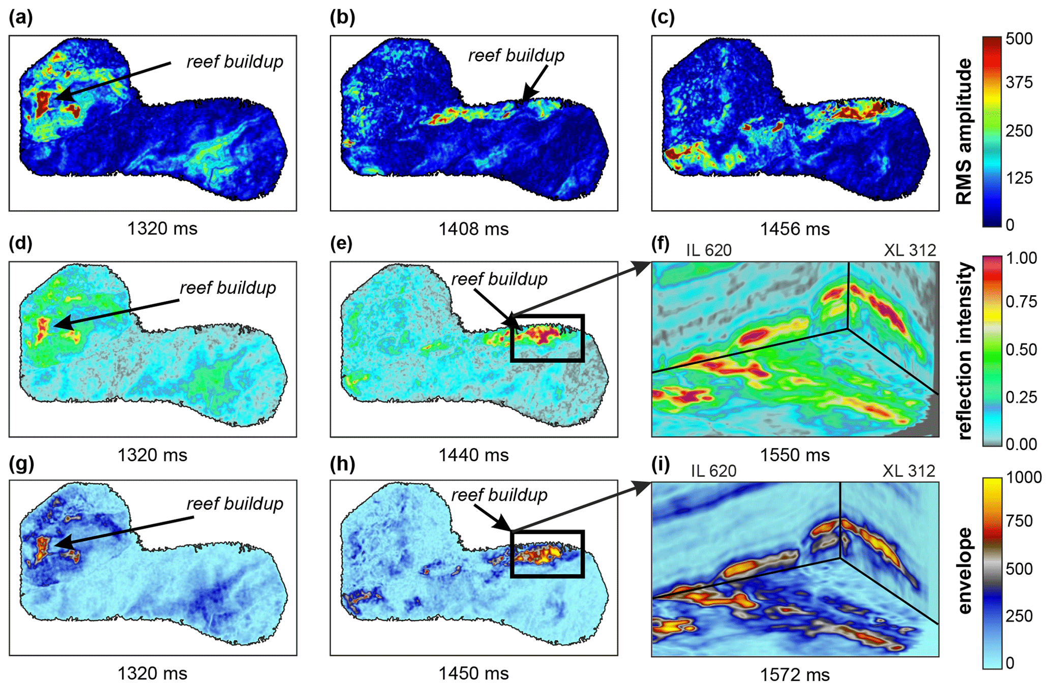
Figure A1Time slices and zoom-ins of the rms amplitude volume (a–c), the reflection intensity volume (d–f), and the envelope volume (g–i). The time slices show locally restricted high-amplitude anomalies interpreted as a possible reef buildups.
One attribute that allows the identification of small variations is the acoustic impedance (Fig. 4). Every reflection changes the amplitude of the returning wave due to a contrast in acoustic impedance, which is the product of the seismic velocity of the wave travelling through the subsurface and the density of the rock (Barclay et al., 2008). Therefore, the reflection amplitudes can be used to invert the data to get impedance values by using e.g. a stochastic seismic amplitude inversion as carried out for our study area by Wadas and von Hartmann (2022). The advantages are that (1) the calculated impedance model delivers a subsurface image with higher resolution due to a reduced tuning effect (Hill, 2005), which allows a more detailed structural and lithological interpretation compared to the classical amplitude attributes; (2) the impedance data can be calibrated with well log data; (3) the data have an increased bandwidth due to implementation of frequencies beyond the seismic bandwidth, e.g. from well logs; (4) it enables the integration of horizons and geological structures; and (5) the derivation of reservoir parameters is based on a strong relationship between acoustic impedance and petrophysical properties (Pendrel and Van Riel, 1997; Hill, 2005; Sarhan, 2017; Gogoi and Chatterjee, 2019).
Phase- and frequency-related attributes
The instantaneous phase (Fig. 5) of the seismic data is calculated by phase = , where f and g are the real and imaginary components of the seismic trace. It measures the phase shift of a specific reflection event, e.g. resulting from a polarity reversal of the reflection coefficient or due to a curved interface (Chopra and Marfurt, 2007). It is calculated sample by sample without regard for the waveform over a specified window. The default window length in Petrel is 33 samples (Schlumberger, 2020), but we chose 15 samples in order to better depict small-scale variations.
The instantaneous frequency is the rate of change of the instantaneous phase from one time sample to the next (inst. frequency = ) over a specified window. The dominant frequency (Fig. 6) is the square of the instantaneous frequency summed with the square of the instantaneous bandwidth, and then the square root of the sum is calculated (Schlumberger, 2020). The dominant frequency thus indicates where the energy of the seismic signal is concentrated in the frequency domain. The chosen window length for both attributes was 15 samples in order to depict small-scale variations. Both frequency attributes are good indicators of bed thickness and changes caused e.g. by fault and fracture zones or differing lithology (Van Tuyl et al., 2018) by distinguishing low- and high-frequency areas (Sarhan, 2017).
Discontinuity-related attributes
For the variance (Fig. 9) a trace-by-trace analysis was performed in order to quantify the dissimilarity of the seismic waveform of neighbouring traces within a specified time window (Bahorich and Farmer, 1995; Marfurt et al., 1998; Wang et al., 2016). The default inline and crossline ranges in Petrel are 3, and we chose a range of 2 in order to enhance small-scale dissimilarities. For vertical smoothing only a mild smoother with 12 samples was applied to prevent smearing of the detected edges. Furthermore, since we wanted to enhance not only faults but also stratigraphic and karstic features, no dip correction or guidance was applied. The attribute chaos is used to map the “chaoticness” of the seismic signal from statistical analysis of dip and azimuth estimates. With directional sigma values the user can define the window radius for calculating the chaoticness of the seismic data, and the larger the sigma, the smoother the result. Therefore, in order to depict small-scale discontinuities a value of 1.0 was chosen for sigma X, sigma Y, and sigma Z (Schlumberger, 2020). Both variance and chaos are commonly utilized to visualize geological features that are characterized by lateral discontinuities, such as stratigraphic terminations or structural lineaments like faults, fractures, dolines, and reef edges (Chopra and Marfurt, 2007). Since both attributes deliver similar results, only variance is shown (Fig. 9).
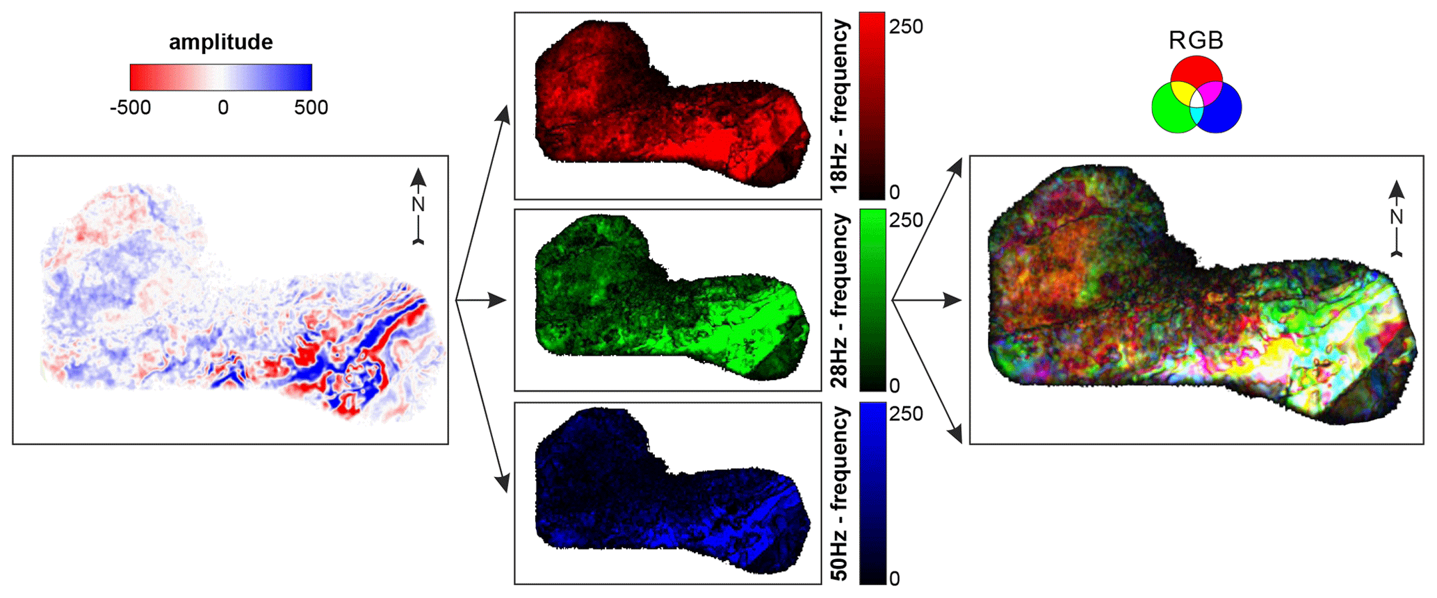
Figure A2Spectral decomposition of the GRAME data with 18 Hz plotted as red, 28 Hz plotted as green, and 50 Hz plotted as blue.
Sweetness
Sweetness (Fig. 8) is the combination of instantaneous frequency and envelope and is described by sweetness = (Radovich and Oliveros, 1998). High sweetness values are correlated with both high envelope and low instantaneous frequencies, whereas low sweetness values result from low envelope and high instantaneous frequencies.
Spectral decomposition
Spectral decomposition (Fig. A2) separates the seismic signal into its frequency components. Three different frequencies are then co-rendered and displayed by RGB colour blending, where frequency 1 is plotted against red, frequency 2 is plotted against green, and frequency 3 is plotted against blue. Since this is an additive colour model, three equally strong signals of the frequency components will result in a white response (Chopra and Marfurt, 2007; Al-Maghlouth et al., 2017). In Petrel a hybrid method, combining a short-time Fourier transform (STFT) and a continuous wavelet transform (CWT), is applied that allows controlling both the vertical and the frequency resolution (Schlumberger, 2020). After iteratively testing different frequency components and their combinations, 18, 28, and 50 Hz were chosen as the best-suited frequencies using three cycles (a small number of oscillations will deliver a better vertical resolution due to the short wavelet).
Curvature
Curvature (Fig. 10) measures how much a seismic reflector is bent. In the case of a planar reflector, the corresponding vectors are parallel, and as a consequence the reflector has zero curvature at this location. In contrast, anticlinal features result in diverging vectors, and the curvature is defined as positive; synclinal features result in converging vectors, and the curvature is defined as negative (Roberts, 2001; Al-Dossary and Marfurt, 2006; Wang et al., 2016). Different curvature types that can be calculated are e.g. Gaussian curvature, mean curvature, minimum and maximum curvature, and most positive and most negative curvature. According to Chopra and Marfurt (2007), the latter are the most suitable to visually correlate with geological features. The most positive curvature is described as the most positive value of all possible normal curvatures at a point, and the most negative curvature is defined as the most negative value of all possible normal curvatures at a given point. The search radius of the algorithm must be selected depending on the research question or the object to be investigated (Roberts, 2001); e.g. a large search radius is needed for detection of regional trends (long wavelength structures) and a small search radius is necessary for small local features (short wavelength structures). Since in our study especially small-scale structures, like buildups and dolines, were investigated, a small search radius was chosen with a vertical radius of 10 samples (the window size is 2 times the vertical radius plus 1) and an inline to crossline radius of 2 (Schlumberger, 2020).
Shape index and curvedness
The formula to calculate the shape index is → S = (Al-Dossary and Marfurt, 2006).
The formula to calculate the curvedness is → C = (Al-Dossary and Marfurt, 2006).
Ant tracking
In the following Schlumberger's patented ant-tracking algorithm and the chosen parameters are described in detail: the initial ant boundary that defines the initial search radius of the agents by a number of voxels (a voxel is defined as the volume around one sample, which in our case relates to the sample rate of the variance cube), in which the agent tries to find a local maximum, was set to two voxels. So if the agent is unable to find a local maximum within this radius, the agent is removed. This close distribution enabled the mapping of small fractures. With the ant-track deviation parameter the maximum allowed deviation while tracking can be determined. For example, a value of 2, as chosen in our study, enables the agent to deviate by two voxels in every direction in order to find the next local maximum (values between zero and three voxels are possible, default is two). If none is found this would be considered an illegal step. With the ant step size the user can define the number of voxels the ant agent can advance during each searching step. As a result, large values allow the agent to search further away for a local maximum, although this will reduce the resolution of the resulting ant-tracking volume. Since our aim was to get a high-resolution volume, the step size was set to two voxels (values between 2 and 10 voxels are possible, default is 3). The user can also specify the number of allowed legal and illegal steps. The legal step parameter describes the number of steps that must contain a valid edge value for the agent to continue. For example, when the agent encounters a valid edge (local maximum), this would represent the first legal step. When the agent continues the search and finds another valid edge, this would be the second legal step. In the case that the user has set this parameter to two legal steps (values between zero and three steps are possible, default is three for passive mode and two for aggressive mode), as was done in this study, this ant track would be considered legitimate and the agent could continue further. If the parameter had been set to three legal steps and no edge had been found after the second legal step, the track would not have been forwarded to the final ant-track volume. The illegal step parameter, which was set to two, defines how far the ant track can continue without finding a local maximum (values between zero and three steps possible, default is one for passive mode and two for aggressive mode). An agent can accumulate illegal steps over time until they represent a significant portion of the entire ant track, leading to uncertainties. To prevent this, a stop criterion given in percent can be defined, which automatically terminates the ant track when the illegal steps exceed the given percentage. In our study we chose a stop criterion of 10 % (values between 0 % and 50 % possible, default is 5 % for passive mode and 10 % for aggressive mode). For the second ant track the same parameters were chosen as for the first ant tracking, except for the initial ant boundary, which was set to four voxels. Afterwards, automatic fault and fracture extraction (Schlumberger, 2020) was used to extract 3D fracture patches from the ant-track volume. The extraction sampling threshold, which sets the minimum signal level from which extraction points were created, was set to the top 30 % of the data, meaning that only the highest ant-track values, representing the sharpest edges, were used for the patch extraction process. Furthermore, the minimum patch size was set to 100 connected voxels.
Table B1Recommended seismic attributes for the detection and parametrization of controlling factors in a deep geothermal carbonate reservoir, such as reefs, karst, faults, and fractures.
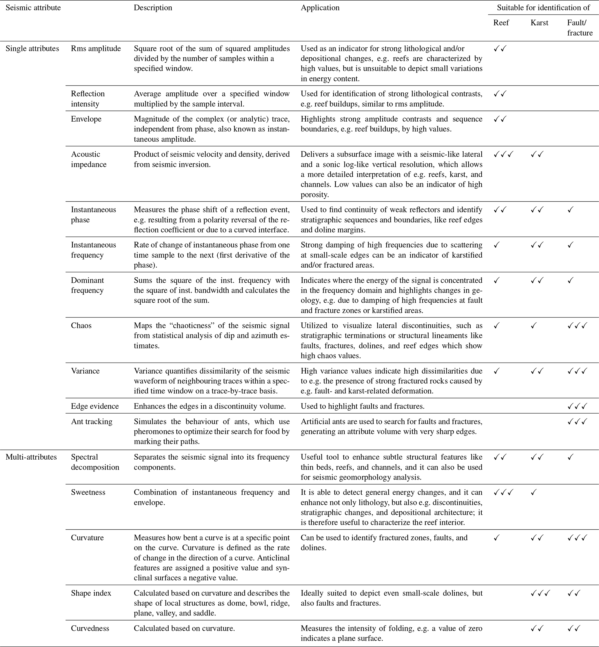
The data that support the findings of this study are available from the Stadtwerke München (SWM) and the Leibniz Institute of Applied Geophysics (LIAG), but restrictions apply to the availability of these data, which were used under license and are therefore not publicly available. Data are, however, available from the authors upon request and with permission of SWM and LIAG.
The data that support the findings of this study were provided by the Stadtwerke München (SWM). Seismic data analysis was carried out by SHW, and image log analysis was carried out by JFK. Interpretation of the seismic analysis results was jointly carried out by all authors. The interpretation and comparison of the fracture orientation results on seismic and well scale were done by SHW, JFK, and MK. SHW prepared and discussed the results with all co-authors. All authors have contributed to the writing of the paper, and SHW, JFK, and MK created the figures.
The contact author has declared that none of the authors has any competing interests.
Publisher's note: Copernicus Publications remains neutral with regard to jurisdictional claims in published maps and institutional affiliations.
We thank Munich City Utilities (Stadtwerke München – SWM) for cooperation and for the seismic and borehole data. Without these data, our study could not have been carried out. We also thank two anonymous referees and the topical editor, Ulrike Werban, for their useful comments that helped to improve the paper.
This research has been supported by the Bundesministerium für Wirtschaft und Energie within the scope of the project REgine, which is part of the joint project GeoMaRe (grant no. 0324332B).
This paper was edited by Ulrike Werban and reviewed by two anonymous referees.
Abdel-Fattah, M. I., Pigott, J. D., and El-Sadek, M. S.: Integrated seismic attributes and stochastic inversion for reservoir characterization: Insights from Wadi field (NE Abu-Gharadig Basin, Egypt), J. Afr. Earth Sci., 161, 1–14, https://doi.org/10.1016/j.jafrearsci.2019.103661, 2020. a, b
Agemar, T., Weber, J., and Schulz, R.: Deep Geothermal Energy Production in Germany, Energies, 7, 4397–4416, https://doi.org/10.3390/en7074397, 2014. a, b
Albesher, Z., Kellogg, J., Hafiza, I., and Saeid, E.: Multi-Attribute Analysis Using Coherency and Ant-Tracking Techniques for Fault and Fracture Detection in La Florida Anticline, Llanos Foothills, Colombia, Geosci., 10, 1–21, https://doi.org/10.3390/geosciences10040154, 2020. a, b, c, d, e, f
Al-Dossary, S. and Marfurt, K.J.: 3D volumetric multispectral estimates of reflector curvature and rotation, Geophysics, 71, P41–P51, https://doi.org/10.1190/1.2242449, 2006. a, b, c, d, e
Al-Halbouni, D., Holohan, E. P., Taheri, A., Schöpfer, M. P. J., Emam, S., and Dahm, T.: Geomechanical modelling of sinkhole development using distinct elements: model verification for a single void space and application to the Dead Sea area, Solid Earth, 9, 1341–1373, https://doi.org/10.5194/se-9-1341-2018, 2018. a, b, c
Al-Maghlouth, M., Szafian, P., and Bell, R.: Characterizing carbonate facies using high-definition frequency decomposition: Case study from North West Australia, Interpretation, 5, SJ49–SJ59, https://doi.org/10.1190/INT-2016-0173.1, 2017. a, b, c
ALT: Advanced Logic Technology, WellCAD – The Universal Borehole Data Toolbox, https://www.alt.lu/wp-content/uploads/WellCAD.pdf (last access: 17 January 2023), 2021. a
Andres, G.: Fränkische Alb und Malmkarst des Molassebeckens – Grundwassergleichenkarte von Bayern 1:500 000 mit Erläuterungen, Schriftenreihe Bayerisches Landesamt für Wasserwirtschaft, 20, 23–25, 1985. a, b
Ashraf, U., Zhu, P., Yasin, Q., Anees, A., Imraz, M., Mangi, H. N., and Shakeel, S.: Classification of reservoir facies using well log and 3D seismic attributes for prospect evaluation and field development: a case study of Sawan gas field, Pakistan, J. Petrol. Sci. Eng., 175, 338–351, https://doi.org/10.1016/j.petrol.2018.12.060, 2019. a
Ashton, M., Dee, S. J., and Wennberg, O. P.: Subseismic-Scale Reservoir Deformation, Geol. Soc. Spec. Publ., https://doi.org/10.1144/SP459, 2018. a
Ba, N. T., Quang, T. P. H., Bao, M. L., and Thang, L. P.: Applying multi-point statistical methods to build the facies model for Oligocene formation, X oil field, Cuu Long basin, J. Pet. Explor. Prod. Technol., 9, 1633–1650, https://doi.org/10.1007/s13202-018-0604-7, 2019. a
Baaske, U. P., Mutti, M., Baioni, F., Bertozzi, G., and Naini, M. A.: Using multi-attribute neural networks classification for seismic carbonate facies mapping: A workflow example from mid-Cretaceous Persian Gulf deposits, Geol. Soc. Spec. Publ., 277, 105–120, https://doi.org/10.1144/GSL.SP.2007.277.01.06, 2007. a
Bachmann, G. H. and Müller, M.: Sedimentary and structural evoluion of the German Molasse Basin, Eclogae Geol. Helv., 85, 519–530, https://doi.org/10.5169/seals-167019, 1992. a, b, c, d, e, f
Bachmann, G. H., Müller, M., and Weggen, K.: Evolution of the Molasse Basin (Germany, Switzerland), Tectonophysics, 137, 77–92, https://doi.org/10.1016/0040-1951(87)90315-5, 1987. a, b, c, d
Backers, T., Kahnt, R., and Stockinger, G.: Structural dominated geothermal reservoir reaction during proppant emplacement in Geretsried, Bavaria, Geomechanics and Tunneling, 15, 58–64, https://doi.org/10.1002/geot.202100091, 2022. a
Bagheri, M. and Riahi, M. A.: Seismic facies analysis from well logs based on supervised classification scheme with different machine learning techniques, Arab. J. Geosci., 8, 7153–7161, https://doi.org/10.1007/s12517-014-1691-5, 2015. a
Bahorich, M. and Farmer, S.: 3-D seismic discontinuity for faults and stratigraphic features: The coherence cube, Lead. Edge, 14, 1053–1058, https://doi.org/10.1190/1.1437077, 1995. a, b
Banerjee, A. and Ahmed Salim, A. M.: Seismic attribute analysis of deep-water Dangerous Grounds in the South China Sea, NW Sabah Platform region, Malaysia, J. Nat. Gas Sci. Eng., 83, 1–15, https://doi.org/10.1016/j.jngse.2020.103534, 2020. a
Barclay, F., Bruun, A., Rasmussen, K. B., Alfaro, J. C., Cooke, A., Cooke, D., Salter, D., Godfrey, R., Lowden, D., McHugo, S., Özdemir, H., Pickering, S., Pineda, F. G., Herwanger, J., Volterrani, S., Murineddu, A., Rasmussen, A., and Roberts, R.: Seismic Inversion: Reading Between the Lines, Oilfield Rev., 20, 42–63, 2008. a, b, c
Barnes, A. E.: Too many seismic attributes?, CSEG Recorder, 31, 1–11, 2006. a
Bauer, J. F., Krumbholz, M., Meier, S., and Tanner, D. C.: Predictability of properties of a fractured geothermal reservoir: the opportunities and limitations of an outcrop analogue study, Geotherm. Energy, 5, 24, https://doi.org/10.1186/s40517-017-0081-0, 2017. a
Bauer, J. F., Krumbholz, M., Luijendijk, E., and Tanner, D. C.: A numerical sensitivity study of how permeability, porosity, geological structure, and hydraulic gradient control the lifetime of a geothermal reservoir, Solid Earth, 10, 2115–2135, https://doi.org/10.5194/se-10-2115-2019, 2019. a, b, c
Beichel, K., Koch, R., and Wolfgramm, M.: Die Analyse von Spülproben zur Lokalisierung von Zuflusszonen in Geothermiebohrungen. Beispiel der Bohrungen Gt Unterhaching 1/1a und 2 (Söddeutschland, Molassebecken, Malm), Geolog. Blätter NO-Bayern, 64, 43–65, 2014. a
Beilecke, T., Krawczyk, C. M., Tanner, D. C., and Ziesch, J.: Near-surface fault detection using high-resolution shear wave reflection seismics at the CO2CRC Otway Project site, Australia, J. Geophys. Res.-Sol. Ea., 121, 1–23, https://doi.org/10.1002/2015JB012668, 2016. a
Benjakul, R., Hollis, C., Robertson, H. A., Sonnenthal, E. L., and Whitaker, F. F.: Understanding controls on hydrothermal dolomitisation: insights from 3D reactive transport modelling of geothermal convection, Solid Earth, 11, 2439–2461, https://doi.org/10.5194/se-11-2439-2020, 2020. a
Birner, J., Fritzer, T., Jodocy, M., Savvatis, A., Schneider, M., and Stober, I.: Hydraulische Eigenschaften des Malmaquifers im Süddeutschen Molassebecken und ihre Bedeutung für die geothermische Erschließung, Z. Geol. Wissenschaft, 40, 133–156, 2012. a, b, c, d
Böhm, F.: Die Lithofazies des Oberjura (Malm) im Großraum München und deren Einfluss auf die tiefengeothermische Nutzung, PhD thesis, Freie Universität Berlin, https://doi.org/10.17169/refubium-6252, 2012. a, b, c, d, e, f, g
Boersma, Q., Athmer, W., Haege, M., Etchebes, M., Haukås, J., and Bertotti, G.: Natural fault and fracture network characterization for the southern Ekofisk field: A case study integrating seismic attribute analysis with image log interpretation, J. Struct. Geol., 141, 1–14, https://doi.org/10.1016/j.jsg.2020.104197, 2020. a, b, c, d, e, f, g, h
Bohnsack, D., Potten, M., Pfrang, D., Wolpert, P., and Zosseder, K.: Porosity–permeability relationship derived from Upper Jurassic carbonate rock cores to assess the regional hydraulic matrix properties of the Malm reservoir in the South German Molasse Basin, Geotherm. Energy, 8, 1–47, https://doi.org/10.1186/s40517-020-00166-9, 2020. a, b, c, d, e
Brcković, A., Kovac̆ević, M., Cvetković, M., Kolenković Moc̆ilac, I., Rukavina, D., and Saftić, B.: Application of artificial neural networks for lithofacies determination based on limited well data, Cent. Eur. Geol., 60, 299–315, https://doi.org/10.1556/24.60.2017.012, 2017. a, b
Bredesen, K., Dalgaard, E., Mathiesen, A., Rasmussen, R., and Balling, N.: Seismic characterization of geothermal sedimentary reservoirs: A field example from the Copenhagen area, Denmark, Interpretation, 8, T275–T291, https://doi.org/10.1190/int-2019-0184.1, 2020. a, b
Cacace, M., Blöcher, G., Watanabe, N., Moeck, I., Börsing, N., Scheck-Wenderoth, M., Kolditz, O., and Huenges, E.: Modelling of fractured carbonate reservoirs: outline of a novel technique via a case study from the Molasse Basin, southern Bavaria, Germany, Environ. Earth Sci., 70, 3585–3602, https://doi.org/10.1007/s12665-013-2402-3, 2013. a, b
Chen, Q. and Sidney, S.: Seismic attribute technology for reservoir forecasting and monitoring, Lead. Edge, 16, 445–456, https://doi.org/10.1190/1.1437657, 1997. a
Chopra, S. and Marfurt, K. J.: Seismic Attributes for Prospect Identification and Reservoir Characterization, Society of Exploration Geophysicists, Tulsa, USA, ISBN 978-1-56080-141-2, 2007. a, b, c, d, e, f, g, h, i, j, k, l, m, n, o, p, q, r, s, t, u, v, w, x, y
Closson, D. and Abou Karaki, N.: Salt karst and tectonics: sinkholes development along tension cracks between parallel strike-slip faults, Dead Sea, Jordan, Earth Surf. Proc. Land., 34, 1408–1421, https://doi.org/10.1002/esp.1829, 2009. a
Da Silva, I. N., Spatti, D. N., Flauzino, R. A., Bartocci Liboni, L. H., and Dos Reis Alves, S. F.: Artificial Neural Networks: A Practical Course, Springer International Publishing, Switzerland, https://doi.org/10.1007/978-3-319-43162-8, 2017. a, b
Del Prete, S., Iovine, G., Parise, M., and Santo, A.: Origin and distribution of different types of sinkholes in the plain areas of Southern Italy, Geodin. Acta, 23, 113–127, https://doi.org/10.3166/ga.23.113-127, 2010. a
Dewett, D. T., Pigott, J. D., and Marfurt, K. J.: A review of seismic attribute taxonomies, discussion of their historical use, and presentation of a seismic attribute communication framework using data analysis concepts, Interpretation, 9, B39–B64, https://doi.org/10.1190/INT-2020-0222.1, 2021. a
Doyen, P. M.: Seismic Reservoir Characterization – An Earth Modelling Perspective, EAGE Publications, ISBN 9073781779, 2007. a
Dunham, R. J.: Classification of carbonate rocks according to depositional textures, in: Classification of Carbonate Rocks – A Symposium, edited by: Ham, W. E., AAPG, Tulsa, USA, ISBN 9781629812366, 1962. a
Dussel, M., Lüschen, E., Thomas, R., Agemar, T., Fritzer, T., Sieblitz, S., Huber, B., Birner, J., and Schulz, R.: Forecast for thermal water use from Upper Jurassic carbonates in theMunich region (South German Molasse Basin), Geothermics, 60, 13–30, https://doi.org/10.1016/j.geothermics.2015.10.010, 2016. a
Ehrenberg, S. N.: Porosity destruction in carbonate platforms, J. Petrol. Geol., 29, 41–52, https://doi.org/10.1111/j.1747-5457.2006.00041.x, 2006. a
Ehrenberg, S. N. and Nadeau, P. H.: Sandstone vs. carbonate petroleum reservoirs: a global perspective on porosity-depth and porosity permeability relationships, AAPG Bull., 89, 435–445, https://doi.org/10.1306/11230404071, 2005. a, b
Eisbacher, G. H.: Molasse – Alpine and Columbian, Geosci. Can., 1, 47–50, 1974. a
Fadel, M., Reinecker, J., Bruss, D., and Moeck, I.: Causes of a premature thermal breakthrough of a hydrothermal project in Germany, Geothermics, 105, 1–18, https://doi.org/10.1016/j.geothermics.2022.102523, 2022. a, b, c
Fang, J., Zhou, F., and Tang, Z.: Discrete Fracture Network Modelling in a Naturally Fractured Carbonate Reservoir in the Jingbei Oilfield, China, Energies, 10, 1–19, https://doi.org/10.3390/en10020183, 2017. a, b, c
Filippova, K., Kozhenkov, A., and Alabushin, A.: Seismic inversion techniques: choice and benefits, First Break, 29, 103–114, 2011. a
Flügel, E.: Microfacies of Carbonate Rocks – Analysis, Interpretation and Application, Springer, Heidelberg, Germany, https://doi.org/10.1007/978-3-642-03796-2, 2010. a, b, c, d
Frisch, W.: Tectonic progradation and plate tectonic evolution of the Alps, Tectonophysics, 60, 121–139, https://doi.org/10.1016/0040-1951(79)90155-0, 1979. a, b
Glassley, W. E.: Geothermal Energy: Renewable Energy and the Environment – 2nd edn., CRC Press, Boca Raton, USA, https://doi.org/10.1201/b17521, 2014. a
Gogoi, T. and Chatterjee, R.: Estimation of petrophysical parameters using seismic inversion and neural network modeling in Upper Assam basin, India, Geosci. Front., 10, 1113–1124, https://doi.org/10.1016/j.gsf.2018.07.002, 2019. a, b
Haq, B. U.: Jurassic Sea-Level Variations: A Reappraisal, GSA Today, 28, 4–10, https://doi.org/10.1130/GSATG359A.1, 2017. a, b
Henderson, J., Purves, S. J., Fisher, G., and Leppard, C.: Delineation of geological elements from RGB color blending of seismic attribute volumes, Lead. Edge, 27, 342–350, https://doi.org/10.1190/1.2896625, 2008. a
Hill, S. J.: Inversion-based thickness determination, Lead. Edge, 25, 477–480, https://doi.org/10.1190/1.1926799, 2005. a, b
Homuth, S.: Aufschlussanalogstudie zur Charakterisierung oberjurassischer geothermischer Karbonatreservoire im Molassebecken, PhD thesis, Technical University Darmstadt, Germany, https://tuprints.ulb.tu-darmstadt.de/4209/ (last access: 7 December 2022), 2014. a
Homuth, S., Göth, A. E., and Sass, I.: Reservoir characterization of the Upper Jurassic geothermal target formations (Molasse Basin, Germany): role of thermofacies as exploration tool, Geotherm. Energy Sci., 3, 41–49, https://doi.org/10.5194/gtes-3-41-2015, 2015. a, b, c, d, e
Huenges, E.: Geothermal Energy Systems: Exploration, Development, and Utilization, Wiley, Weinheim, Germany, ISBN 978-3-527-64461-2, 2010. a
Jaglan, H., Quayyum, F., and Huck, H.: Unconventional seismic attributes for fracture characterization, First Break, 33, 101–109, https://doi.org/10.3997/1365-2397.33.3.79520, 2015. a, b
Janson, X. and Madriz, D. D.: Geomodelling of carbonate mounds using two-point and multipoint statistics, Geol. Soc. of London, Spec. Publ., 370, 229–246, https://doi.org/10.1144/SP370.5, 2012. a
Jolley, S. J., Barr, D., Walsh, J. J., and Knipe, R. J.: Structurally complex reservoirs: an introduction. Geol. Soc. Spec. Publ., 292, 1–24, https://doi.org/10.1144/SP292.1, 2007. a
Kendall, C. and Schlager, W.: Caronates and relative changes in sea level, Mar. Geol., 44, 181–212, https://doi.org/10.1016/0025-3227(81)90118-3, 1981. a, b, c
Koch, R.: Dolomit und Dolomit-Zerfall im Malm Süddeutschlands – Verbreitung, Bildungsmodelle, Dolomit-Karst, Laichinger Höhlenfreund, 46, 75–92, 2011. a, b, c
Koch, R., Bachmann, G. H. B., and Müller, M.: Fazies des Oberen Jura (Malm) der Bohrungen Scherstetten 1 und 2 (Molasse-Becken, Süddeutschland) und ihre Bedeutung für die geothermische Exploration, Z. Geol. Wissenschaft, 38, 327–351, 2010. a, b
Konrad, F., Savvatis, A., Wellmann, F., and Zosseder, K.: Hydraulic behavior of fault zones in pump tests of geothermal wells: a parametric analysis using numerical simulations for the Upper Jurassic aquifer of the North Alpine Foreland Basin, Geotherm. Energy, 7, 1–28, https://doi.org/10.1186/s40517-019-0137-4, 2019. a, b
Korneva, I., Bastesen, E., Corlett, H., Eker, A., Hirani, J., Hollis, C., Gawthorpe, R. L., Roteveatn, A., and Taylor, R.: The effects of dolomitization on petrophysical properties and fracture distribution within rift-related carbonates (Hammam Faraun Fault Block, Suez Rift, Egypt), J. Struct. Geol., 108, 108–120, https://doi.org/10.1016/j.jsg.2017.06.005, 2018. a
Lai, J., Wang, G., Wang, S., Cao, J., Li, M., Pang, X., Han, C., Fan, X., Yang, L., He, Z., and Qin, Z.: A review on the applications of image logs in structural analysis and sedimentary characterization, Mar. Petrol. Geol., 95, 139–166, https://doi.org/10.1016/j.marpetgeo.2018.04.020, 2018. a
Lake, L. W. and Srinivasan, S.: Statistical scale-up of reservoir properties: concepts and applications, J. Petrol. Sci. Eng., 44, 27–39, https://doi.org/10.1016/j.petrol.2004.02.003, 2004. a
Lemcke, K.: Das bayerische Alpenvorland vor der Eiszeit: Erdgeschichte-Bau-Bodenschätze, Stuttgart: Schweizerbart, ISBN 978-3-510-65135-1, 1988. a, b, c, d
Li, S., Wang, D., and Zhang, M.: Influence of upscaling on identification of reservoir fluid properties using seismic-scale elastic constants, Sci. Rep., 9, 1–11, https://doi.org/10.1038/s41598-019-49559-2, 2019. a
Liu, G., Zeng, L., Han, C., Ostadhassan, M., Lyu, W., Wang, Q., Zhu, J., and Hou, F.: Natural Fractures in Carbonate Basement Reservoirs of the Jizhong Sub-Basin, Bohai Bay Basin, China: Key Aspects Favoring Oil Production, Energies, 13, 1–23, https://doi.org/10.3390/en13184635, 2020. a
Lohr, T.: Seismic and sub-seismic deformation on different scales in the NW German Basin, PhD Thesis, Technical University Berlin, Berlin, Germany, https://doi.org/10.17169/refubium-16413, 2008. a
Loza Espejel, R., Alves, T. M., and Blenkinsop T. G.: Multi-scale fracture network characterisation on carbonate platforms, J. Struct. Geol., 140, 1–23, https://doi.org/10.1016/j.jsg.2020.104160, 2020. a, b, c
Lucia, F. J.: Carbonate reservoir characterization: an integrated approach, Berlin: Springer, https://doi.org/10.1007/978-3-540-72742-2, 2007. a, b, c, d, e, f, g, h
Lüschen, E., Wolfgramm, M., Fritzer, T., Dussel, M., Thomas, R., and Schulz, R.: 3D seismic survey explores geothermal targets for reservoir characterization at Unterhaching, Munich, Germany, Geothermics, 50, 167–179, https://doi.org/10.1016/j.geothermics.2013.09.007, 2014. a
Machel, H. G.: Concepts and models of dolomitization: a critical reappraisal, Geol. Soc. Spec. Publ., 235, 7–63, 2004. a, b, c, d, e
Marfurt, K. J.: Techniques and best practices in multiattribute display, Interpretation, 3, B1–B23, https://doi.org/10.1190/INT-2014-0133.1, 2015. a, b, c, d, e, f
Marfurt, K. J. and Kirlin, R. L.: Narrow‐band spectral analysis and thin‐bed tuning, Geophysics, 66, 1274–1283, https://doi.org/10.1190/1.1487075, 2001. a, b
Marfurt, K. J. and Alves, T. M.: Pitfalls and limitations in seismic attribute interpretation of tectonic features, Interpretation, 3, SB5–SB15, https://doi.org/10.1190/INT-2014-0122.1, 2015. a, b, c
Marfurt, K. J., Kirlin, R. J., Farmer, S. L., and Bahorich, M. S.: 3-D seismic attributes using a semblance‐based coherency algorithm, Geophysics, 63, 1150–1165, https://doi.org/10.1190/1.1444415, 1998. a, b, c
Méndez, J. N., Jin, Q., González, M., Zhang, X., Lobo, C., Boateng C. D., and Zambrano, M.: Fracture characterization and modeling of karsted carbonate reservoirs: A case study in Tahe oilfield, Tarim Basin (western China), Mar. Petrol. Geol., 112, 1–17, https://doi.org/10.1016/j.marpetgeo.2019.104104, 2020. a, b
Moeck, I. S.: Catalog of geothermal play types based on geologic controls, Renew. Sust. Energ. Rev., 37, 867–882, https://doi.org/10.1016/j.rser.2014.05.032, 2014. a
Moeck, I., Dussel, M., Weber, J., Schintgen, T., and Wolfgramm, M.: Geothermal play typing in Germany, case study Molasse Basin: a modern concept to categorise geothermal resources related to crustal permeability, Neth. J. Geosci., 98, 1–10, https://doi.org/10.1017/njg.2019.12, 2020. a, b, c
Mountjoy, E. W. and Marquez, X. M.: Predicting Reservoir Properties in Dolomites: Upper Devonian Leduc Buildups, Deep Alberta Basin, in: Reservoir quality prediction in sandstones and carbonates, edited by: Kupecz, J. A., Gluyas, J., and Bloch, S., AAPG Memoir, 69, 267–306, 1997. a
Mraz, E.: Reservoir characterization to improve exploration concepts of the Upper Jurassic in the Southern Bavarian Molasse Basin, PhD thesis, Technische Universität München, http://nbn-resolving.de/urn/resolver.pl?urn:nbn:de:bvb:91-diss-20190430-1464081-1-6 (last access: 15 November 2022), 2019. a, b, c, d, e, f, g, h, i
Mraz, E., Moeck, I., Bissmann, S., and Hild, S.: Multiphase fossil normal faults as geothermal exploration targets in the Western Bavarian Molasse Basin: Case study Mauerstetten, Z. Deut. Ges. Geowiss., 169, 389–411, 2018. a
Parise, M. and Lollino P.: A preliminary analysis of failure mechanisms in karst and man-made underground caves in Southern Italy, Geomorphology, 134, 132–143, https://doi.org/10.1016/j.geomorph.2011.06.008, 2011. a
Pendrel, J. and Van Riel, P.: Methodology for Seismic Inversion, A Western Canadian Reef Example, CSEG Recorder, 22, 1–16, 1997. a
Pendrel, J.: Seismic Inversion – The Best Tool for Reservoir Characterization, CSEG Recorder, 26, 1–12, 2001. a, b
Pieńkowski, G., Schudack, M. E., Bosák, P., Enay, R., Feldman-Olszewska, A., Golonka, J., Gutowski, J., Herngreen, G. F. W., Jordan, P., Krobicki, M., Lathuiliere, B., Leinfelder, R. R., Michalik, J., Mönnig, E., Noe-Nygaard, N., Pálfy, J., Pint, A., Rasser, M. W., Reisdorf, A. G., Schmid, D. U., Schweigert, G., Surlyk, F., Wetzel, A., and Wong, T. E.: Jurassic, in: The Geology of Central Europe Volume 2: Mesozoic and Cenozoic, edited by: McCann, T., The Geological Society, London, 823–922, https://doi.org/10.1144/CEV2P, 2008. a, b, c
Playton, T. E., Janson, X., and Kerans, C.: Carbonate slopes, in: Facies Models 4, edited by: James, N. P. and Dalrymple, R. W., Geological Association of Canada, ISBN 9781897095508, 2010. a
Pomar, L. and Ward, W. C.: Sea-Level Changes, Carbonate Production and Platform Architecture: The Llucmajor Platform, Mallorca, Spain, in: Sequence Stratigraphy and Depositional Response to Eustatic, Tectonic and Climatic Forcing. Coastal Systems and Continental Margins, edited by: Haq, B. U., Vol. 1, Springer, Dordrecht, Netherlands, https://doi.org/10.1007/978-94-015-8583-5, 1995. a
Pussak, M., Bauer, K., Stiller, M., and Bujakowski, W.: Improved 3D seismic attribute mapping by CRS stacking instead of NMO stacking: Application to a geothermal reservoir in the Polish Basin, J. Appl. Geophys., 103, 186–198, https://doi.org/10.1016/j.jappgeo.2014.01.020, 2014. a
Radovich, B. J. and Oliveros, R. B.: 3-D sequence interpretation of seismic instantaneous attributes from the Gorgon Field, Lead. Edge, 17, 1286–1293, https://doi.org/10.1190/1.1438125, 1998. a, b
Raines, M. A. and Dewers, T. A.: Dedolomitization as a driving mechanism for karst generation in Permian Blaine Formation, southwestern Oklahoma, USA, Carbonate. Evaporite., 12, 24–31, https://doi.org/10.1007/BF03175799, 1997. a
Rawal, K., Wang, Z.-M., and Hu, L.: Exploring the Geomechanics of Sinkholes: A Numerical Simulation Approach, Geo-Chicago 14–16 August, Chicago, Illinois, USA, 1–11, https://doi.org/10.1061/9780784480120.039, 2016. a
Reinhold, C.: Multiple episodes of dolomitization and dolomiterecrystallization during shallow burial in Upper Jurassic shelf carbonates: eastern Swabian Alb, southern Germany, Sediment. Geol., 121, 71–95, 1998. a, b, c, d, e, f, g, h, i, j
Roberts, A.: Curvature attributes and their application to 3D interpreted horizons, First Break, 19, 85–100, https://doi.org/10.1046/j.0263-5046.2001.00142.x, 2001. a, b, c, d, e, f, g
Roden, R., Smith, T., and Sacrey, D.: Geologic pattern recognition from seismic attributes: Principal component analysis and self-organizing maps, Interpretation, 3, SAE59–SAE83, https://doi.org/10.1190/INT-2015-0037.1, 2015. a, b
Saggaf, M. M., Toksöz, N. M., and Marhoon, M. I.: Seismic facies classification and identification by competitive neural networks, Geophysics, 68, 1984–1999, https://doi.org/10.1190/1.1635052, 2003. a
Sajed, O. K. M. and Glover, P. W. J.: Dolomitisation, cementation and reservoir quality in three Jurassic and Cretaceous carbonate reservoirs in north-western Iraq, Mar. Petrol. Geol., 115, 1–20, https://doi.org/10.1016/j.marpetgeo.2020.104256, 2020. a
Salmi, E. F., Nazem, M., and Giacomini, A.: A Numerical Investigation of Sinkhole Subsidence Development over Shallow Excavations in Tectonised Weak Rocks: The Dolaei Tunnel's Excavation Case, Geotech. Geol. Eng., 35, 1685–1716, https://doi.org/10.1007/s10706-017-0202-3, 2017. a
Sammut, C. and Webb, G. I.: Encyclopedia of Machine Learning and Data Mining, Springer, New York, USA, https://doi.org/10.1007/978-1-4899-7687-1, 2017. a
Sarhan, M. A.: The efficiency of seismic attributes to differentiate between massive and non-massive carbonate successions for hydrocarbon exploration activity, NRIAG J. Astron. Geophys., 6, 311–325, https://doi.org/10.1016/j.nrjag.2017.06.003, 2017. a, b, c, d, e, f, g
Schlumberger: FMI Fullbore Formation MicroImage, Schlumberger Educational Services, Houston, Texas, USA, 2004. a, b
Schlumberger: Petrel Guru – Software Manual, 2020. a, b, c, d, e, f, g, h, i, j, k, l, m, n, o, p
Schmid, D. U., Leinfelder, R. R., and Schweigert, G.: Stratigraphy and palaeoenvironments of the Upper Jurassic of Southern Germany – a review, Proceedings of the 4th International Symposium on Lithographic Limestone and Plattenkalk, Eichstätt, Germany 12–18 September 2005, 31–41, 2005. a, b, c
Schmoker, J. W. and Halley, R. B.: Carbonate porosity versus depth: a predictable relation for south Florida, Am. Assoc. Petr. Geol. B., 66, 2561–2570, 1982. a
Schneider-Löbens, C., Wuttke, M., Backers, T., and Krawczyk, C. M.: Numerical modeling approach of sinkhole propagation using the eXtended FEM code roxol, EGU General Assembly 2015, Vienna, http://meetingorganizer.copernicus.org/EGU2015/EGU2015-12230-2.pdf (last access: 13 September 2017), 2015. a
Sell, A., Buness, H., Tanner, D., Ziesch, J., and Weller, A.: FD modelling of deeply-buried paleo-dolines underneath the city of Munich, EAGE Near Surface Geoscience Conference and Exhibition, 1st Conference on Geophysics for Geothermal and Renewable Energy Storage, The Hague, Netherlands, 8–12 September 2019, 2019. a
Shiau, J. and Hassan, M. M.: Numerical modelling of three-dimensional sinkhole stability using finite different method, Innov. Infr. Solutions, 6, 1–9, https://doi.org/10.1007/s41062-021-00559-0, 2021. a
Shipilin, V., Tanner, D. C., von Hartmann, H., and Moeck, I.: Multiphase, decoupled faulting in the southern German Molasse Basin – evidence from 3-D seismic data, Solid Earth, 11, 2097–2117, https://doi.org/10.5194/se-11-2097-2020, 2020. a
Skirius, C., Nissen, S., Haskell, N., Marfurt, K., Hadley, S., Ternes, D., Michel, K., Reglar, I., D'Amico, D., Deliencourt, F., Romero, T., D'Angelo, R., and Brown, B.: 3-D seismic attributes applied to carbonates, Lead. Edge, 18, 384–393, https://doi.org/10.1190/1.1438303, 1999. a
Steidtmann, E.: The Evolution of Limestone and Dolomite, J. Geol., 19, 323–345, https://www.jstor.org/stable/pdf/30060008.pdf (last access: 14 January 2023), 1911. a
Stier, P. and Prestel, R.: Der Malmkarst im süddeutschen Molassebecken – Ein hydrogeologischer Überblick in: Hydrogeothermische Energiebilanz und Grundwasserhaushalt des Malmkarstes im süddeutschen Molassebecken, Bayerisches Landesamt für Wasserwirtschaft (Bay. LFW), München, Geologisches Landesamt Baden-Württemberg (LGRB), Freiburg, Schlussbericht zum BMFT-FE-Vorhaben, 1991. a
Taner, M. T.: Seismic attributes, CSEG Recorder, 26, 49–56, 2001. a, b, c
Toublanc, A., Renaud, S., Sylte, J. E., Clausen, C .K., Eiben, T., and Nådland, G.: Ekofisk Field: fracture permeability evaluation and implementation in the flow model, Petrol. Geosci., 11, 321–330, https://doi.org/10.1144/1354-079304-622, 2005. a, b
Tucker, M. E. and Wright, V. P.: Carbonate Sedimentology, Blackwell Publishing, Oxford, UK, https://doi.org/10.1002/9781444314175, 1990. a
Van Tuyl, J., Alves, T. M., and Cherns, L.: Geometric and depositional responses of carbonate buildups to Miocene sea level and regional tectonics offshore northwest Australia, Mar. Petrol. Geol., 94, 144–165, https://doi.org/10.1016/j.marpetgeo.2018.02.034, 2018. a, b
Veeken, P. C. H.: Seismic Exploration Vol. 37 – Seismic Stratigraphy, Basin Analysis and Reservoir Characterization, Elsevier, Oxford, UK, ISBN 978-0-08-045311-8, 2007. a, b, c, d, e
von Hartmann, H., Buness, H., Krawczyk, C. M., and Schulz, R.: 3-D seismic analysis of a carbonate platform in the Molasse Basin – reef distribution and internal separation with seismic attributes, Tectonophysics, 572–573, 16–25, https://doi.org/10.1016/j.tecto.2012.06.033, 2012. a
Wadas, S. H., Tanner, D. C., Polom, U., and Krawczyk, C. M.: Structural analysis of S-wave seismics around an urban sinkhole: evidence of enhanced dissolution in a strike-slip fault zone, Nat. Hazards Earth Syst. Sci., 17, 2335–2350, https://doi.org/10.5194/nhess-17-2335-2017, 2017. a
Wadas, S. H., Tschache, S., Polom, U., and Krawczyk. C. M.: Sinkhole imaging and identification of fractures with SH-wave reflection seismic, Proceedings of the 15th Multidisciplinary Conference on Sinkholes and the Engineering and Environmental Impacts of Karst, Shepherdstown, West Virginia, USA, 2–6 April 2018, 307–314, https://doi.org/10.5038/9780991000982.1003, 2018. a
Wadas, S. H. and von Hartmann, H.: Porosity estimation of a geothermal carbonate reservoir in the German Molasse Basin based on seismic amplitude inversion, Geotherm. Energy, 10, 1–40, https://doi.org/10.1186/s40517-022-00223-5, 2022. a, b, c, d, e, f, g, h, i, j, k, l, m, n, o, p, q
Waltham, T., Bell, F. G., and Culshaw, M.: Sinkholes and Subsidence – Karst and Cavernous Rocks in Engineering and Construction, Springer-Verlag, Berlin, Germany, ISBN 3642058515, 2005. a
Wang, Y., Eichkitz, C. G., Schrelechner, M. G., Heinemann, G., Davis, J. C., and Gharsalla, M.: Seismic attributes for description of reef growth and channel system evolution – Case study of Intisar E, Libya, Interpretation, 4, SB1–SB11, https://doi.org/10.1190/INT-2015-0017.1, 2016. a, b, c, d, e, f, g
Williams, R. M., Pascual-Cebrian, E., Gutmanis, J. C., and Paton, G. S.: Closing the seismic resolution gap of fractures through seismic and image-log analysis, a North Sea case study, Interpretation, 5, SJ21–SJ30, https://doi.org/10.1190/INT-2016-0163.1, 2017. a
Wolfgramm, M., Dussel, M., Koch, R., Lüschen, E., Schulz, R., and Thomas, R.: Identifikation und Charakterisierung der Zuflusszonen im Malm des Molassebeckens nach petrographisch-faziellen und geophysikalischen Daten, Proceedings – Der Geothermiekongress, Bochum, Germany, 15–17 November 2011, 1–14, 2011. a, b
Xu, X., Chen, Q., Chu, C., Li, G., Liu, C., and Shi, Z.: Tectonic evolution and paleokarstification of carbonate rocks in the Paleozoic Tarim Basin, Carbonate. Evaporite., 32, 487–496, https://doi.org/10.1007/s13146-016-0307-4, 2017. a
Zahmatkesh, I., Kadkhodaie, A., Soleimani, B., and Azarpour, M.: Integration of well log-derived facies and 3D seismic attributes for seismic facies mapping: A case study from mansuri oil field, SW Iran, J. Petrol. Sci. Eng., 202, 1–20, https://doi.org/10.1016/j.petrol.2021.108563, 2021. a, b
Zhao, T., Jayaram, V., Roy, A., and Marfurt, K. J.: A comparison of classification techniques for seismic facies recognition, Interpretation, 3, SAE29–SAE58, https://doi.org/10.1190/INT-2015-0044.1, 2015. a, b
Ziegler, P. A.: Late Cretaceous and Cenozoic intraplate compressional deformations in the Alpine foreland – a geodynamic model, Tectonophysics, 137, 399–420, https://doi.org/10.1016/0040-1951(87)90330-1, 1987. a
Ziesch, J.: Prediction of seismic and sub-seismic deformation to ensure carbon traps in the Otway Basin, PhD Thesis, Australia, Technical University Berlin, Berlin, Germany, https://doi.org/10.14279/depositonce-5386, 2016. a
Ziesch, J.: 3D-Strukturanalyse und Retrodeformation, in: Endbericht GeoParaMol – Bestimmung von relevanten Parametern zur faziellen Interpretation des Malm und Modellierung des thermisch-hydraulischen Langzeitverhaltens, Project report for the German Ministry of Economic Affairs, Chap. 4.3, 51–63, https://doi.org/10.2314/KXP:1678714100, 2019. a, b, c, d, e, f, g