Unbiased statistical length analysis of linear features: adapting survival analysis to geological applications

A proper quantitative statistical characterization of fracture length or height is of paramount importance when analysing outcrops of fractured rocks. Past literature suggests adopting a non-parametric approach, such as circular scanlines, for the unbiased estimation of the fracture-length mean value. This is due to the fact that, in the past, estimating any type of statistical distribution was difficult and there was no real interest in defining precise parametrical models. However, due to the recent rise in popularity of digital outcrop models (DOMs) and of stochastic discrete fracture networks (DFNs), there is an increasing demand for distribution-based solutions that output a correct estimation of parameters for a given proposed model (e.g. mean and standard deviation). This change in demand highlights in the geological literature the absence of properly structured theoretical works on this topic. Our methodology, presented for the first time in this contribution, represents a powerful alternative to non-parametrical methods, aimed at specifically treating censoring bias and obtaining an unbiased trace-length statistical model. As our first objective, we propose to tackle the censoring bias by applying survival analysis techniques: a branch of statistics focused on modelling time-to-event data and correctly estimating model parameters with data affected by censoring. As a second objective, we propose a novel approach for selecting the most representative parametric model. We combine a direct visual approach and the calculation of four statistics to quantify how well proposed models reflect the data. We apply survival analysis to correctly estimate statistical parameters of a censored length dataset in three different case studies and show the effects of the censoring percentage on parametrical estimations that do not use this paradigm. The presented analyses are carried out using an open-source Python package called FracAbility, which we purposefully created to carry out the described workflow (https://github.com/gecos-lab/FracAbility, last access: 8 September 2024).

1 Introduction

Fractured rock masses are complex systems composed of intact rock and discontinuities (Hoek, 1983). Characterizing the statistical distribution of three-dimensional (3D) geometrical properties of such discontinuities (e.g. aperture, roughness, area, orientation, height $/$ length ratio) is fundamental for understanding and modelling mechanical and hydraulic properties of rock masses and fluid–rock interaction. The recent increase in computing power and the emergence of new approaches based on digital outcrop models (DOMs) allow the extraction of large datasets and facilitate the sampling of properties instead of just their estimation (Bistacchi et al., 2015; Tavani et al., 2016; Healy et al., 2017; Thiele et al., 2017; Marrett et al., 2018; Nyberg et al., 2018; Bistacchi et al., 2020; Martinelli et al., 2020; Bistacchi et al., 2022; Mittempergher and Bistacchi, 2022; Storti et al., 2022). The need for a more rigorous statistical approach to structural data analysis is also motivated by the popularization of stochastic discrete fracture networks (DFNs) as a modelling approach for rock masses. In DFNs, discontinuities are represented, in a simplified way, as finite planar surfaces, generally rectangular, polygonal, or elliptical (Cacas et al., 1990; Dershowitz et al., 1992; Tavakkoli et al., 2009; Hyman et al., 2015). In fact, stochastic algorithms used to generate these surfaces are guided by statistical distributions obtained from field or well data or are assumed based on some prior knowledge (Andersson et al., 1984; Cacas et al., 1990; Davy et al., 2018). For example, DFNs where fractures are represented as rectangular surfaces (the most common implementation) require the definition of fracture size via parametric distributions of length (measured along strike) and height (measured along dip) or, alternatively, length and length $/$ height ratio (Hyman et al., 2015). However, it is worth noting that DFNs are not the only viable approach to modelling fractured rock volumes. Other methods, such as tensorial approximations (Brown and Bruhn, 1998; Suzuki et al., 1998) based on the crack tensor measure (Oda, 1983), are also used (Healy et al., 2017) and, with details depending on the implementation, require similar parameters in input.

The main obstacle that geologists encounter while trying to characterize a fractured rock volume is the impossibility of directly measuring the 3D properties of discontinuities, since only indirect geophysical methods may provide complete 3D datasets. However, imaging discontinuities with geophysical methods are strongly limited by spatial resolution and/or by the absence of contrast in the physical properties investigated by a particular technique (Martinelli et al., 2020). Therefore, a vast body of research focuses on the characterization of properties of discontinuity traces or lineaments, i.e. the two-dimensional (2D) intersections of 3D discontinuity surfaces with the outcrop surface or with topography (Dershowitz and Herda, 1992; Bonnet et al., 2001; Manzocchi, 2002; Bistacchi et al., 2011; Sanderson and Nixon, 2015; Bistacchi et al., 2020; Martinelli et al., 2020; Storti et al., 2022). In this contribution, we focus on the problem of defining accurate and unbiased length (or height) distributions based on data collected on DOMs. In any given outcrop, lineament length measurements will always be affected by four main biases: length (i.e. size), censoring, truncation, and orientation (Baecher, 1983). The correction of these biases has been thoroughly researched, and the standard solution currently adopted by many authors is based on circular scanlines (Mauldon, 1998; Zhang and Einstein, 1998; Mauldon et al., 2001; Rohrbaugh et al., 2002). The method consists of drawing a circle directly on the outcrop or on an image and counting the intersections of the circle with lineaments. With a chain of assumptions, defining an indirect relationship between mean length and the intersections of lineaments with the scanline, an unbiased non-parametric estimation of mean length, fracture density, and intensity can be obtained (Mauldon et al., 2001). Thanks to its simple implementation in the field, this technique is widely used; however, it has an important limitation: lineament lengths are never directly measured. For this reason, analysis carried out with the circular scanline method yields estimates of mean length values but is unable to provide a complete characterization of the lineament length distribution and therefore lacks any real statistical significance. Despite this problem, the popularity of this method was motivated by the fact that, in the past, without modern digital imaging techniques, length data acquisition was slow and tedious; thus datasets were usually small. Moreover, calculating the length and estimating any distribution other than the exponential was difficult and computationally intensive (Baecher and Lanney, 1978; Baecher, 1980), and, due to limitations in early algorithms used to generate stochastic fracture networks, there was no real interest in using precise distribution parameters in input. These limitations have mostly been overcome by modern characterization methods; thus new tools and techniques based on the maximum likelihood estimator (MLE), such as FracPaQ (Healy et al., 2017; Rizzo et al., 2017), have been developed, enabling researchers to apply quantitative statistical inference on dense digital datasets.

Our methodology, presented for the first time in this contribution, represents a powerful alternative to circular scanline methods to treat specifically the censoring bias and to obtain unbiased trace length statistical models. This specific bias is defined when, for some traces, one or both ends cannot be seen due to the limited size of the outcrop (Baecher and Lanney, 1978). This effect is present from thin section to satellite image scale, and it is caused by the inability to see beyond the study area (i.e. thin-section limits, outcrop extension; Mauldon et al., 2001). From a statistical point of view, this problem is analogous to the censoring bias affecting some medical, biological, and engineering datasets, and the techniques used in these disciplines to solve or limit the effects of this bias go under the names of survival analysis, life testing, or reliability analysis (Kaplan and Meier, 1958; Leung et al., 1997; Lawless, 2003; Cox, 2017; Karim and Islam, 2019). Even though, in these disciplines, the recorded random variables are time spans (e.g. lifetime of a patient, time to failure of a mechanical part), we demonstrate that this statistical technique can also be adapted to length measurements. Measuring length is straightforward with dedicated code or with a simple GIS software; however, applying survival analysis and fitting robust unbiased parametric statistical distributions needs a more detailed treatment. As the main topic of this contribution, we propose to adapt survival/reliability analysis techniques to correctly account for censored lengths and estimate robust trace length distributions derived from DOMs. Furthermore, we define a quantitative methodology to select the most representative estimated statistical model (i.e. parametric distribution) from a list of proposed models. The theory and techniques presented in this paper are available as an open-source Python package called FracAbility that accepts shapefiles as input and allows one to carry out a complete and unbiased statistical analysis workflow for fracture-length data (https://github.com/gecos-lab/FracAbility. last access: 8 September 2024).

2 Fracture surveys and terminology

A discontinuity in a rock mass can be defined as a surface across which a material has lost its cohesion or was originally discontinuous. This definition thus includes faults, fractures, foliations, stylolites, compaction or deformation bands, and bedding interfaces. Fractures are classified as shear or tensional fractures. Tensional fractures, when possible, can be further divided into joints when empty or veins when filled by minerals (Twiss and Moores, 2007; Davis et al., 2012). This distinction, however, is often difficult to make without an in-depth field and sample validation, since some fractures may have hybrid fill attributes and may be only partly filled with inconspicuous mineral deposits and thus resemble joints. Moreover, the degree of fill may depend on fracture width so that small fractures resemble veins (Laubach et al., 2019). Although three-dimensional by nature, most of the times discontinuities are mapped as 2D lineaments or traces over a surface. These lineaments are the intersections of such discontinuities with an exposed surface, such as the topography, an outcrop, a borehole, or a sample. In this work, following a common usage in outcrop studies, the term fracture is used as a generic term to indicate any type of discontinuity trace. Fractures with the same formation age, kinematics, and orientation can be grouped into families or sets. Multiple fracture sets present within an area form a fracture network or system (Davis et al., 2012).

Additionally, fracture networks present two other fundamental components: boundaries and nodes (Fig. 1a). Boundaries are the limits of the sampling area, at scales from thin sections to satellite images, within which the sampled fracture traces are assumed to be complete. Ideally, boundaries are strictly convex; however, this is often not the case. Boundaries often show tight bends, coves, and holes, and the final shapes are mostly controlled by localized alteration, anthropogenic activity, vegetation, etc. (Fig. 1b).

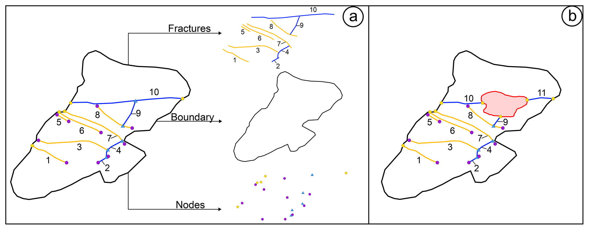
Figure 1 Panel (a) shows an example of a simple fracture network and its components. Panel (b) shows a modified version of the boundary with a “hole” (in red) in which no interpretation can be carried out. The presence of these holes can increase the number of censored fractures and introduce uncertainty into the interpretation, splitting fractures into multiple pieces (i.e. fracture 10 is split in two).

Nodes are points in the network that define how fractures interact or do not interact with other elements of the network (other fractures, boundary, holes). Nodes can be classified by the number and type of segments (branches) that insist on the given point (Sanderson and Nixon, 2015) (Fig. 2):

• Isolated I nodes are connected to only one branch belonging to a fracture.

• Y/T and X nodes are respectively connected to three and four branches belonging to two fractures.

• “Boundary” B nodes are connected to one branch belonging to a fracture and two branches belonging to the boundary.

Node elements describe useful hydraulic properties of a fractured rock mass (Gueguen et al., 1991; Manzocchi, 2002; Sanderson and Nixon, 2015).
In a non-porous rock with all open fractures, a network with a prevalence of I nodes is less connected; thus fluid flow is usually more restrained. Conversely, both Y/T and X nodes increase the connectivity of the network and thus increase both fluid flow and the permeability. However, sometimes this is indeed not the case, e.g. sealed faults and opening-mode fractures (Forstner and Laubach, 2022). Moreover, if a rock is porous, then length becomes the key parameter for controlling fluid flow; thus, even in a network with only I nodes, length can markedly augment fluid flow (Philip et al., 2005). Additionally, nodes give important chronological information about the network. I nodes indicate that fractures terminate within the observational boundary and that they do not end or cross with other fractures. Y/T nodes can be evidence of either abutting or cross-cutting relationships of non-coeval discontinuities; the former is relevant for discontinuities with no displacement, while the latter applies to discontinuities with visible displacement. X nodes represent a mutual cross-cutting relationship, and the chronological interpretation depends also on other observations. Finally, B nodes identify whether a fracture is complete or censored and, as such, define if measured properties along a trace are also complete or incomplete. These nodes could be regarded as a sort of equivalent of the U (undefined) nodes in Nyberg et al. (2018), however, with a slightly different meaning and more precise definition.

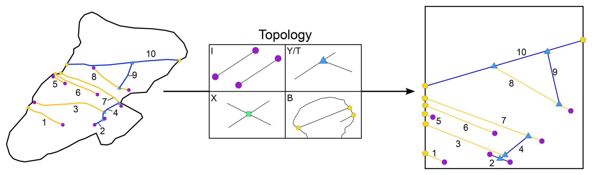
Figure 2 Topological abstraction of the simple fracture network in Fig. 1 following the described node classification.

3 Statistical modelling of censored length data

Having a length dataset, there is usually the necessity of estimating the parameters of one or multiple statistical distributions. When doing so, censoring is inevitable, as the area within which measures are carried out will always be limited. Then, how can we carry out an unbiased estimation of such parameters? On the one hand, common and simplistic approaches, such as ignoring censoring (i.e. regarding censored lengths as if they were complete) or excluding censored measurements (i.e. cherry-picking only non-censored data), should be avoided, as they will always lead to an underestimation of the model parameters (see Discussion for a more in-depth analysis). On the other hand, circular scanline methods offer an unbiased estimate of the mean length; however, being non-parametric, they yield neither the distribution type (e.g. normal, exponential) nor distribution shape parameters (e.g. standard deviation, variance). This in turn makes the estimate's use quite limited and not apt for downstream statistical modelling applications (such as DFNs). To solve these problems, we propose using survival analysis, a specialized field of statistics, developed to deal with censored data. Survival analysis focuses on the analysis of time of occurrence until an event of interest (Kalbfleisch and Prentice, 2002). Although, in literature, the terms survival times, time to failure, and (more generally) lifetimes (Lawless, 2003) seem to imply that time is the only valid variable, any non-negative continuous variable, such as length, can be valid (Kalbfleisch and Prentice, 2002; Lawless, 2003). The advantage of survival analysis over the other methods discussed above is that it regards censored data as a valid data point and as a carrier of the information that the event did not occur up to the censoring time. This is a necessary shift in perspective that allows an unbiased estimation of statistical models that will be described in this paper. We will start by describing the theory of survival analysis in function of time, then we will show how the same theory can be applied in space to sets of length or distance measurements.

3.1 Survival analysis theory and standard terminology

Since this technique is rooted in medical and biological applications, the nomenclature from this type of literature is carried along. The event of interest (for which we measure the time to event) is often defined as death, while a loss indicates that the observation has been lost because it was hindered by a secondary event, called a censoring event (Kaplan and Meier, 1958). Censoring events can be classified as three main types depending on when censoring happens in respect of the observation period (Karim and Islam, 2019) (Fig. 3):

1. Right censoring. The event happens after the end of the study period; thus the partial lifetime of the event is observed.

2. Left censoring. The event happens before the start of the study; thus it is not observed.

3. Interval censoring. The event happens somewhere between observation intervals within the study period because it was not possible to continuously monitor the occurrence of the event.

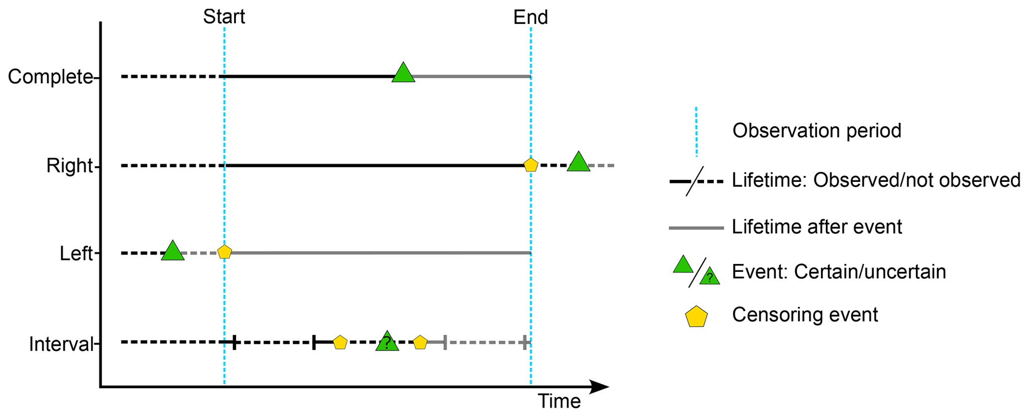
Figure 3 Different censoring types in a fixed observation period. Right censoring is defined when the event happens after the end of the study. Left censoring occurs when the event happens before the start of the study. Interval censoring happens somewhere between observation intervals within the study period.

The most treated and common type is right censoring, which can be further divided into the following (Fig. 4):

1. Single censoring. When there is an imposed end time equal for all events (i.e. controlled loss).

2. Random censoring. When each measured event is characterized by a random censoring event (i.e. accidental loss).

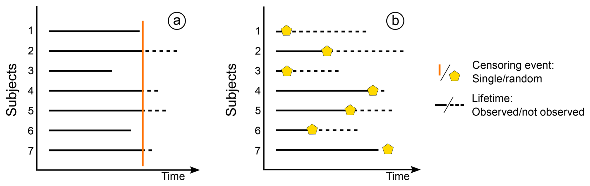
Figure 4 Different right-censoring types for the same seven subject experiments. Panel (a) represents single censoring, where events 1, 3, and 6 are complete measurements, while the remaining events are censored at time C. In panel (b), only event 7 is complete, while the others are all censored at different times.

3.2 The survival curve and the Kaplan–Meier estimator

A fundamental assumption in survival analysis is the independence of the right-censoring mechanisms, i.e. the assumption that the probability of occurrence of the event does not depend on the censoring mechanism (Kalbfleisch and Prentice, 2002; Lawless, 2003; Kleinbaum and Klein, 2012). Independent censoring is also called non-informative censoring, as it does not affect inference and only indicates that the lifetime exceeds the censoring time (Kalbfleisch and Prentice, 2002). This assumption is the basis of the non-parametric Kaplan–Meier estimator of the survival function (SF), i.e. the population probability that X_i exceeds a given value x (Kaplan and Meier, 1958; Kalbfleisch and Prentice, 2002):

$$\begin{array}{}\text{(1)}& \text{SF}\left(x\right)=P(X_i>x).\end{array}$$

The survival function is often called the complementary cumulative function, since it adds to 1 with the cumulative distribution function (CDF):

$$\begin{array}{}\text{(2)}& \text{CDF}\left(x\right)=P(X_i\le x)=\mathrm{1}-P(X_i>x)=\mathrm{1}-\text{SF}\left(x\right).\end{array}$$

The non-parametric Kaplan–Meier estimator $\widehat{P}\left(x\right)$ is defined by ordering N values of complete x_co and censored x_ce data by increasing magnitude, with $x_{\mathrm{1}}\le x_{\mathrm{2}}\le \mathrm{\dots }\le x_N$, such that (Kaplan and Meier, 1958; Kalbfleisch and Prentice, 2002)

$$\begin{array}{}\text{(3)}& \widehat{P}\left(x\right)=\prod _r{\displaystyle \frac{N-r}{N-r+\mathrm{1}}},\end{array}$$

where r is the indexes in which the complete values are smaller than a value x (i.e. x_co≤x).

Therefore, $\widehat{P}\left(x\right)$ is a step function that (Fig. 5)

1. remains constant in any given time interval where no new events are recorded or where censoring occurs;

2. decreases by a degree (step) depending on the number of events that occur in a time interval.

Empirical survival curves are fundamental for representing, comparing, and understanding the survival rates of different censored datasets. The curve's steepness is directly proportional to the survival rate, and the median of the (random) survival time (i.e. time value corresponding to a 50 % chance of survival) can be used as a simple indicator to compare different survival curves.

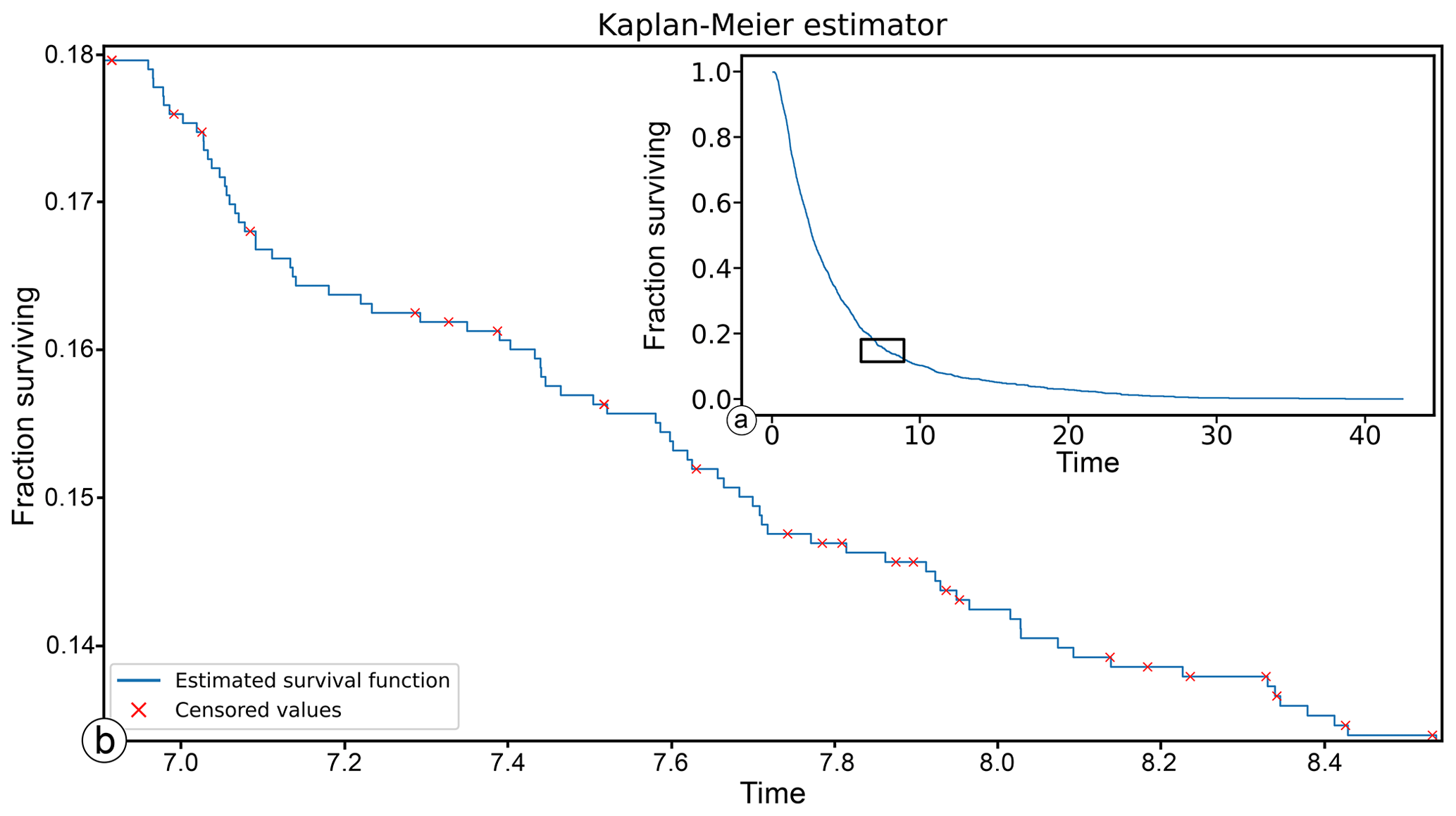
Figure 5 An example of the Kaplan–Meier estimated survival curve. In panel (a), the estimated curve seems continuous; however, when zooming in (red rectangle in panel a), one can see it is a step function (b). The red crosses indicate the censoring events and show how the function never jumps at these values.

3.3 The time–length dimensional shift

Since length is, as time, a non-negative continuous variable, it is theoretically possible to apply survival analysis techniques to length datasets by considering (Fig. 6)

1. the complete fracture trace length analogous to the lifetime;

2. the event as the end (death) of a trace, marked by a node (I and/or Y/T nodes in the case of complete traces);

3. the study area, defined by its boundary, analogous to the study period;

4. the censored event to be the intersection between the fracture trace and the boundary (marked by a B node).

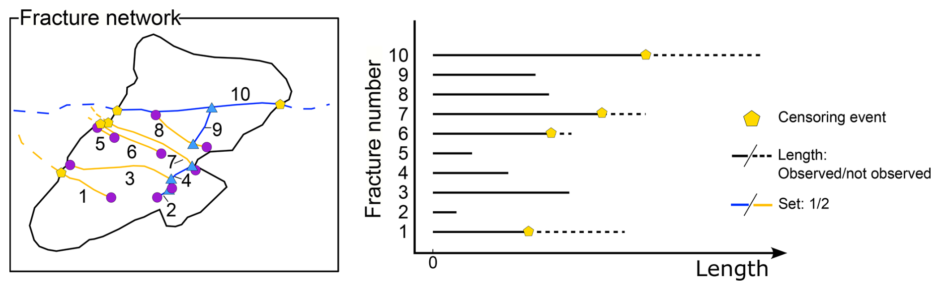
Figure 6 Censoring effect on an example of a simple fracture network and corresponding survival diagram. The survival diagram is a 1D representation of the fracture length. On the y axis the fracture number is indicated, and on the x axis the length is represented. Solid lines indicate the actual measured length, while dashed lines indicate the possible continuation of the fracture. Yellow pentagons represent the censoring event given by the intersection of the fracture with the boundary.

By applying the definitions of the different types of censoring (described in Sect. 3.1) to our specific application, it is reasonable to assume that only random censoring occurs in trace length analysis. Moreover, censoring is non-informative, since the boundary is the product of secondary events (i.e. alteration, erosion, debris covering parts of the outcrop, vegetation, human activity) that occur after fracture genesis and thus do not inform the occurrence of the event (see Discussion for a more in-depth analysis).

3.4 Unbiased MLE model estimation for censored data

Considering that the censored event does not modify the probability of occurrence of the measured event, survival analysts try to solve the problem of estimating a parametric statistical model (i.e. distribution) by using optimization algorithms such as linear regression or the maximum likelihood estimator (MLE). Both methods are valid; however, in these types of applications, MLE is most used; thus we will discuss this technique in more detail.

Given a statistical parametric model with density g(x,θ) (i.e. an assumed theoretical distribution) and a sample x of size n, the main objective of MLE is to estimate the parameters $\widehat{\mathit{\theta }}$ such that the observations x are the most likely under $\mathit{g}(\mathit{x},\widehat{\mathit{\theta }})$ (Burnham and Anderson, 2002, 2004; Karim and Islam, 2019).

In the simplest one-dimensional (1D) case (estimation of the parameter of a one-parameter distribution), the likelihood can be described as a chain product of probabilities carried out on all n individuals in the following sample:

$$\begin{array}{}\text{(4)}& L\left(\mathit{\theta }\right|x,g)=\prod _{i=\mathrm{1}}^{n}g(x_i,\widehat{\mathit{\theta }}).\end{array}$$

Given the fixed (assumed) distribution type g with parameter θ and a sample x, the likelihood will be the product of all the probabilities $\mathit{g}({\mathit{x}}_i,\widehat{\mathit{\theta }})$, i.e. the distribution's probability density function (PDF) calculated at value x_i (P(θ|x_i)). In practice, since g and x are fixed, the likelihood is a function only of the distribution parameter θ. The maximum of this function will be $\widehat{\mathit{\theta }}$, i.e. the parameter that maximizes the likelihood for that model type and data combination. This process can be extended to estimate multiple parameters, increasing the complexity, but the core concept remains unaltered. However, Eq. (4) is valid only for complete datasets because the probabilities associated with right-censored data cannot be calculated using the PDF. To solve this problem, it is possible to calculate the MLE for censored datasets, under the assumption of random censoring, using the model's survival function (SF) S(θ|x_i) instead of the PDF for the censored data (Karim and Islam, 2019):

$$\begin{array}{}\text{(5)}& L\left(\mathit{\theta }\right|x,g)=\prod _{i=\mathrm{1}}^{n}P(\mathit{\theta }|x_i{)}^{{\mathit{\delta }}_i}\times S(\mathit{\theta }|x_i{)}^{\mathrm{1}-{\mathit{\delta }}_i},\end{array}$$

where δ is an on–off switch for complete (δ=1) or censored (δ=0) values. In other words, when data are censored, we use the probability information that the individual survived up to the censoring event, given by the survival function.

MLE is a consistent (i.e. estimation approaches the population parameter as sample size increases) and efficient (i.e. lowest variance) estimator (Enders, 2005); however, it has its limitations. For example, if the model has more than one parameter, the weight of influence of each parameter is not known; thus it is difficult to know which parameter controls the fit. Moreover, simplistic MLE algorithms output a single likelihood value, with a possibility that the optimization gets trapped in a local minimum. This ultimately leads to questioning whether the estimated parameter or combination of parameters is the absolute best or if there are other more optimal solutions. These (and other) problems culminate to an even greater uncertainty related to the choice of the distribution, as an infinite variety of functions can be used for the same dataset. These uncertainties tie nicely to the following subsection discussing model selection comparison criteria and how we propose to solve this problem.

3.5 Model selection

With a series of fitted models, it is important to understand which model better represents the data. In the geological literature, this is usually achieved using a specific type of null hypothesis test defined as a goodness-of-fit (GOF) test (i.e. Storti et al., 2022). These types of tests, in general, do not identify the best-fitting distribution among a set of possible distributions. A GOF test takes a distribution L and the sample data and tells if the model L is not plausible; that is, if the probability of drawing such a set of data, from a population of distribution L, is too small. This means that more than one distribution may be deemed plausible and that the conclusion is strong only when a distribution is an unlikely model for the data. Moreover, GOF tests usually have underlying assumptions that, if ignored, undermine the test's accuracy (Storti et al., 2022). For example, the Kolmogorov–Smirnov test (Kolmogorov, 1933) is biased if the parameters of the tested distribution are estimated from the data (Bistacchi et al., 2020). As an alternative to GOF tests, we propose a combined visual and quantitative approach that guides the researcher in an informed choice of the most representative model out of a list of sensible candidates. By sensible candidates, we mean those models that make physical sense for the case study. For example, for fracture lengths, a power law can be considered a sensible candidate, since it describes an observed pattern of fracture self-similarity. A lognormal is also an equally sensible candidate because of the effect of truncation. Conversely, a normal distribution is not very sensible, since values in the left tail can be negative. Thus, for a normal model, either the average length is very high and the standard deviation is very low or a truncated normal should be tested. In the Case studies section, we will cover different models, purposefully adding non-sensible models (such as a standard normal) to showcase the model selection workflow.

3.5.1 A visual approach using the probability integral transform (PIT)

The probability integral transform (PIT) is a well-known transformation of continuous distributions which converts random variables with continuous distribution to standard uniform distributed random variables (Fisher, 1990), given

1. a random variable Y,

2. F_Y as the CDF of Y,

3. Z=F_Y(Y) as the PIT of Y and a standard uniform random variable.

This means that, given a random sample X, sampled from a population with distribution Y, the transformed sample Z=F_Y(X) has, with large probability, an empirical distribution which is close to the standard uniform distribution. Clearly, if we transform X with another distribution W, which is not the true distribution of the population, then F_W(X) is not uniformly distributed. This observation provides a visual tool to compare different fits: indeed, suppose that sample X might have been sampled from a population of distribution Y or W. We may compute the two transformed samples Z₁=F_Y(X) and Z₂=F_W(X): if X was drawn from distribution Y, then the empirical distribution of Z₁ is likely to be close to the standard uniform, while, if the true distribution was W, then we expect that Z₂, instead of Z₁, would be close to the standard uniform. A synthetic example of PIT is presented in Fig. 7. A random sample X of 10 000 (non-censored) measures is extracted from a standard normal distribution Y (Fig. 7a). The exponential Y_E model (hypothesis) has been fit with an MLE to the random sample. Figure 7b and c represent the empirical frequency histogram and the empirical CDF (ECDF) of Z for both models (Z_N=F_n(X) and Z_E=F_e(X)). Both figures show that the normal estimated model follows a standard uniform, while the exponential model does not. The ECDF visualization of Fig. 7c is preferred over the simple frequency binning of Fig. 7b, since multiple models can be tidily represented with the reference uniform distribution appearing as the diagonal of the plot. The closer the ECDF of Z is to the diagonal of the plot, the closer the fit is to the true underlying model. Values in the PIT plot that are below the diagonal indicate an overestimation of the model's CDF in respect to the empirical cumulative. Conversely, values that are above the diagonal will result in an underestimation of the model's CDF. Hence, the PIT provides a simple visual, yet powerful, method to estimate which parametric model better fits the empirical data.

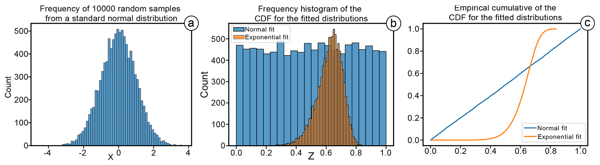
Figure 7 Synthetic example of the probability integral transform. Panel (a) shows 10 000 random samples X drawn from a standard normal distribution Y. Panel (b) shows the frequency distribution of Z from two different models (hypotheses): normal (Y_N) and exponential (Y_E). Panel (c) shows the empirical cumulative of Z for both models. In panels (b) and (c), it is possible to observe the effect of the probability integral transform. In panel (b), the empirical frequency histogram of the normal model is remarkably close to a uniform distribution, while the exponential model is not. This is visualized much more clearly in panel (c), where the normal model is the closest to the diagonal line y=x (i.e. the standard uniform).

3.5.2 A quantitative approach using distances

While the PIT visual approach is very intuitive, we propose also using a quantitative approach, calculating four different statistics. The first is the Akaike information criterion (AIC) (Akaike, 1974), which, by using the result of the MLE, quantifies the distance between the true natural phenomena and the estimated model as

$$\begin{array}{}\text{(6)}& \text{AIC}=\mathrm{2}k-\mathrm{2}\ln \mathcal{L}\left(\widehat{\mathit{\theta }}\right),\end{array}$$

where k is the number of parameters used by the model (i.e. the dimension of the parameter vector) and $\widehat{\mathit{\theta }}$ is the k-dimensional parameter vector that maximizes the likelihood of the model (ℒ).
This formulation outputs a real number (either positive or negative) which should be small as the distance between the true population and the model decreases. If multiple models are tested, then it is possible and advised to calculate the Δ_i parameter, i.e. the distances between the different models to the best-scoring one (AIC_min):

$$\begin{array}{}\text{(7)}& {\mathrm{\Delta }}_i={\text{AIC}}_i-{\mathrm{AIC}}_{\min },\end{array}$$

where i is the index of the proposed model.

From Δ_i it is possible to obtain the weight of evidence (w_i) of the given model with the following formula:

$$\begin{array}{}\text{(8)}& w_i={\displaystyle \frac{e^{-{\mathrm{\Delta }}_i/\mathrm{2}}}{{\sum }_{r=\mathrm{1}}^R{e}^{-{\mathrm{\Delta }}_R/\mathrm{2}}}},\end{array}$$

where R is the total number of tested models (i.e. models deemed reasonable by the researcher).

The weight of evidence outputs a value between [0;1] that represents, in a set of proposed hypotheses, how likely it is that the model comes close to the true underlying process. The closer to 1, the more likely it is that, in the pool of candidates, the model represents the true underlying process (Burnham and Anderson, 2004). Since AIC and the derived formulas are directly based on the MLE, they are affected by the same limitations discussed in Sect. 3.4 (Akaike, 1974). We thus propose calculating three different distances between the model and the data (Kim, 2019). Usually, distances are calculated by comparing the empirical cumulative frequency with the cumulative frequency of the model; however, the data are censored; thus we use the empirical cumulative frequency estimated from Kaplan–Meier. Moreover, Kim (2019) proposes to calculate the distances using the data transformed with PIT (i.e. Z=F_y(X)). We would like to highlight that, purely from the point of view of the calculation, the distances are the same with or without using the transform; however, with PIT, the data are “normalized”; thus the different models are compared over the same scale (0, 1). Equation (3) then can be rewritten as

$$\begin{array}{}\text{(9)}& {\widehat{G}}_n\left(z\right)=\left\{\begin{array}{ll}\mathrm{0},& z<Z_{\mathrm{1}}\\ \mathrm{1}-{\prod }_{Z_r\le z}(\frac{N-r}{N-r+\mathrm{1}}{)}^{{\mathit{\delta }}_r},& z\le Z_N\\ \mathrm{1},& z>Z_N\end{array}\right.,\end{array}$$

where r is the indexes of each data point and δ_r is the same on–off switch of Eq. (5).

Kim (2019) then proposes to calculate

• the Kolmogorov–Smirnov statistic (DC_n), representing the maximum distance between the two cumulative curves (Kolmogorov, 1933; Smirnov, 1939);

• The Koziol and Green statistic (Ψ²), representing the sum of squared distances between the two cumulative curves (Koziol and Green, 1976);

• the Anderson–Darling statistic (${\text{AC}}_n^{\mathrm{2}}$), representing the weighted sum of squared distances between the two cumulative curves, imparting more weight than the Kolmogorov–Smirnov on tail observation (the closer to 0 or 1, the higher the weight; Anderson and Darling, 1954).

The three sets of statistics can be modified to accommodate the presence of censored data by using the Kaplan–Meier estimator.

The Kolmogorov–Smirnov statistic is generally calculated as

$$\begin{array}{}\text{(10)}& {\text{DC}}_n=max({\text{DC}}_n^{+},{\text{DC}}_n^{-}),\end{array}$$

where, with censored data,

$$\begin{array}{}\text{(10a)}& {\displaystyle }{\text{DC}}_n^{+}& {\displaystyle }=max\left({\widehat{\mathit{G}}}_n\right({\mathit{Z}}_r)-{\mathit{Z}}_r),\text{(10b)}& {\displaystyle }{\text{DC}}_n^{-}& {\displaystyle }=max({\mathit{Z}}_{r+\mathrm{1}}-{\widehat{\mathit{G}}}_n({\mathit{Z}}_r\left)\right).\end{array}$$

The Koziol–Green statistic is a generalization of the Cramér–von Mises statistic (Koziol and Green, 1976):

$$\begin{array}{}\text{(11)}& {\mathrm{\Psi }}^{\mathrm{2}}=N\underset{\mathrm{0}}{\overset{\mathrm{1}}{\int }}\left({\widehat{G}}_n\right(z)-z{)}^{\mathrm{2}}\mathrm{d}z,\end{array}$$

which, considering censored data, can be written as (Appendix 2 in Koziol and Green, 1976)

$$\begin{array}{}\text{(11a)}& \begin{array}{rl}{\mathrm{\Psi }}^{\mathrm{2}}& ={\displaystyle \frac{\mathrm{1}}{\mathrm{3}}}N+N\sum _{r=\mathrm{1}}^N{\widehat{G}}_n\left(Z_r\right)\times \left(Z_{r+\mathrm{1}}\right)-Z_r\\ & \times \left[{\widehat{G}}_n\right(Z_r)-(Z_{r+\mathrm{1}}-Z_r\left)\right].\end{array}\end{array}$$

Finally, the Anderson–Darling distance (Anderson and Darling, 1954), generally defined as

$$\begin{array}{}\text{(12)}& {\text{AC}}_n^{\mathrm{2}}=N\underset{\mathrm{0}}{\overset{\mathrm{1}}{\int }}{\displaystyle \frac{\left({\widehat{G}}_n\right(z)-z{)}^{\mathrm{2}}}{z(\mathrm{1}-z)}}\mathrm{d}z,\end{array}$$

where $\frac{\mathrm{1}}{z(\mathrm{1}-z)}$ is the weight, can be calculated accounting for censoring as a finite sum (Kim, 2019):

$$\begin{array}{}\text{(12a)}& \begin{array}{rl}{\text{AC}}_n^{\mathrm{2}}=& N\sum _{r=\mathrm{1}}^{N-\mathrm{1}}\left({\widehat{G}}_n\right(Z_r){)}^{\mathrm{2}}\times (-\ln (\mathrm{1}-Z_{r+\mathrm{1}})+\ln \left(Z_{r+\mathrm{1}}\right)\\ & +N\times (\mathrm{1}-Z_r)-\ln \left(Z_r\right))+\\ -\mathrm{2}& N\sum _{r=\mathrm{1}}^{N-\mathrm{1}}\left({\widehat{G}}_n\right(Z_r\left)\right)\times (-\ln (\mathrm{1}-Z_{r+\mathrm{1}})+\ln (\mathrm{1}-Z_r\left)\right)+\\ -& N\times \ln (\mathrm{1}-Z_N)+N\times \ln \left(Z_N\right)+N.\end{array}\end{array}$$

Once these distances are calculated for each model, we propose to rank the models independently for each distance (from minimum to maximum). If all distances converge (i.e. for the same model, the same rank is assigned), then we regard this as sufficient proof for the overall ranking of the model in the list. By comparing multiple rankings, even if the calculated distances are ranked differently, it is still possible to make a sensible guided choice, for example, by using the PIT representation together with the mean ranking position or by following a specific type of distance.

4 Case studies

We demonstrate the applicability of the discussed theory by using the FracAbility package in three different case studies. The first case study focuses on the characterization of a very regular and densely fractured fracture network with a simple boundary geometry. The second focuses on analysing a typical average-quality outcrop, with multiple fracture sets and complex boundary geometry. Finally, the third case study presents an application with spacing analysis to demonstrate that any type of length can (and must) be corrected from right-censoring bias. We propose to test six statistical models of length, frequently adopted in the literature (Bonnet et al., 2001) or used in stochastic DFNs:

• Lognormal

• Truncated power law (power law in the following)

• Normal

• Weibull

• Exponential

• Two-parameter gamma (gamma in the following).

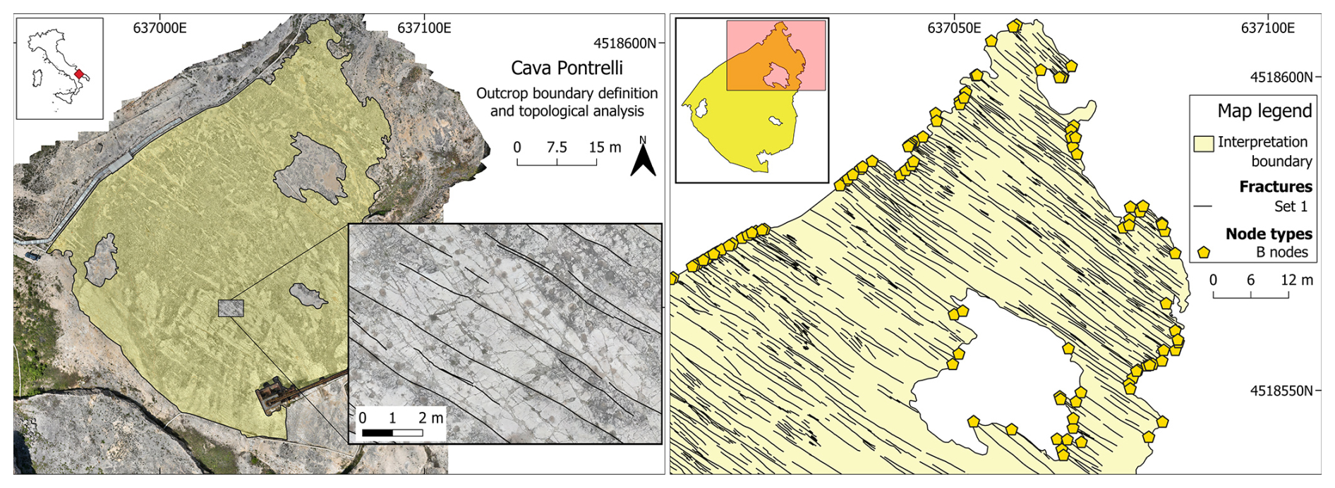
Figure 8 Overview maps of the first case study area. Pictured on the left is a general overview of the area with the boundary geometry overlaid on the orthophoto and a small sample of the digitized fracture set. Pictured on the right is a subarea of the quarry with the boundary, fracture traces, and boundary nodes (yellow pentagons).

4.1 First case study: Cava Pontrelli, Puglia (IT)

This first case study focuses on the analysis of a single NW–SE-striking fracture set present in an abandoned quarry near the town of Altamura in Puglia (Italy). The study area is located on the Apulian Platform, representing the forebulge of the southern part of the fold and thrust belt of the Apennines (Vai and Martini, 2001; Patacca and Scandone, 2007). The outcrop is characterized by an extensive horizontal pavement of about 18.000 m², showing densely fractured Cretaceous platform limestone of the Altamura Limestone Formation (Ricchetti and Luperto Sinni, 1979). The continuous maintenance that followed the discovery of thousands of dinosaur footprints on the quarry pavement (Nicosia et al., 1999) made it possible to obtain an exceptionally clean outcrop surface. This in turn resulted in the definition of a simple boundary geometry (with a couple of interpretational holes) and the digitalization of a very regular and dense fracture network (1941 fractures). The combination of these factors led to a very low percentage of censoring, with only 8.9 % of the total fractures being censored (Fig. 8).

We applied survival analysis as implemented in FracAbility, and, in Fig. 9, the resulting PIT plot is shown. The most representative model appears to be the lognormal, confirmed by all the distances calculated in Table 1 (ordered by ascending Akaike scores; see Fig. 10 for a summary of the fit). Figure 9 shows that the PIT of the lognormal model is quite linear, with gentle undulations indicating a slight underestimation for lengths between 1 and 2 m (accounting for 20 % of the measures) and a slight overestimation for lengths between 3.5 and 6.5 m (accounting for another 20 % of the measures). For the calculated distance scores, the lognormal is followed by the gamma and Weibull models; however, the rank scores of these last two models are not uniform. While the Koziol and Green distance favours the gamma model, the Anderson–Darling distance favours the Weibull model. Finally, the power-law and normal models rank lowest in comparison to the other models, indicating that they are less able to represent the dataset.

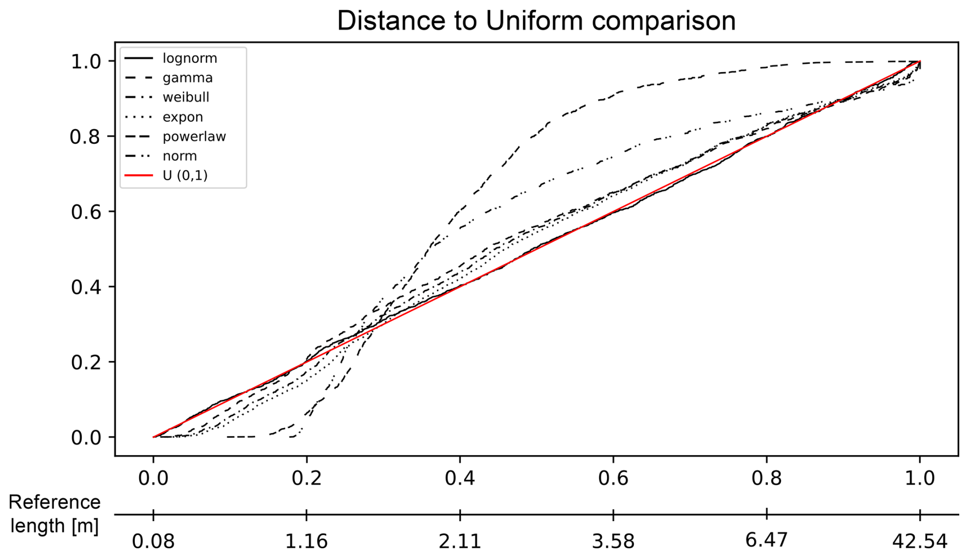
Figure 9 PIT visualization for the proposed length models in the Pontrelli quarry. The red line represents the reference U(0,1): the closer the model line is to this reference line, the more representative the model. For this dataset, the lognormal model is the most representative, following the reference line almost perfectly, with some minor underestimation between 1.16 and 2.11 m and overestimation between 3.58 and 6.47 m.

Table 1 Models' distance tables and ranking score tables for the Pontrelli quarry. The closer to 0, the better. For this dataset, the lognormal is the most representative of the data in all the different distances, while the power-law and normal models are the least representative. The positions of the other models in between are less certain (especially the gamma and exponential).

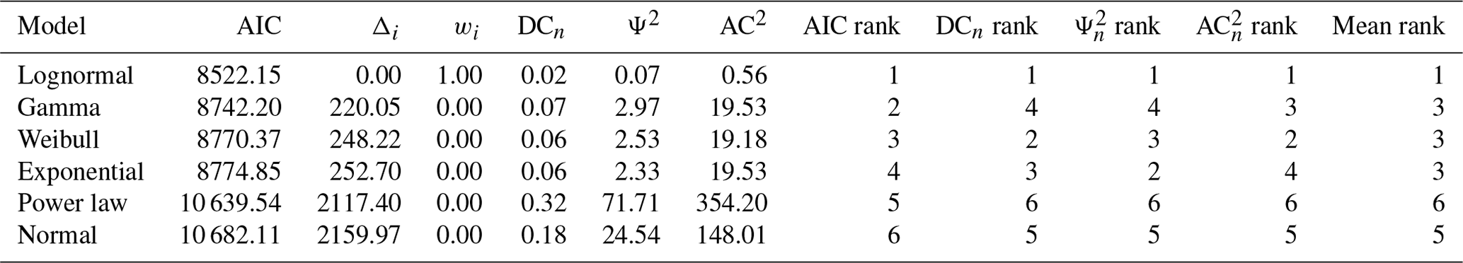
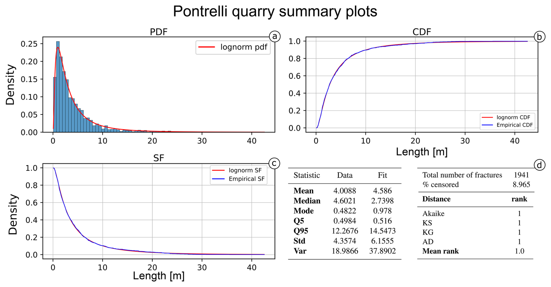
Figure 10 Summary of the best-fitting model (lognormal) for the Pontrelli quarry dataset. (a) The probability density function against the histogram of the dataset. (b) The cumulative distribution function and (c) the survival function against the empirical counterparts calculated with the Kaplan–Meier estimator. (d) The summary table of the main statistics for the data (e.g. sample mean, sample variance) compared with the estimated model.

4.2 Second case study: Colle Salza, Valle d'Aosta (IT)

The second case study focuses on the analysis of a less ideal, albeit more realistic, outcrop. The study area is located in the basement of the Western Alps (Dal Piaz et al., 2003), on paragneiss of the Monte Rosa Nappe (Dal Piaz and Lombardo, 1986). The outcrop is cross-cut by several brittle fractures, Tertiary in age (Bistacchi and Massironi, 2000), and is characterized by a main central area of 1234 m² and two secondary smaller satellite areas of 9 and 3 m². The boundary geometry is highly concave, thus leading to a high censoring fraction of fracture traces. Moreover, the outcrop is exposed on top of a small topographical height with a slightly ellipsoidal shape due to glacial erosion (i.e. a roche moutonnée), with the main axis directed NW–SE. This leads to an inevitable deformation of the orthophoto (and thus of the measured lengths) along the extremities of the analysed area. The analysed fractures are subdivided in two main sets, striking NE–SW (Set 1) and NW–SE (Set 2), conforming to the general trend of the area for brittle deformation (Bistacchi et al., 2000; Bistacchi and Massironi, 2000; Bistacchi et al., 2001). The total number of fractures is 1718 (24.7 % censored), while, set-wise, the number of fractures is 692 (24.3 % censored) for Set 1 and 1026 (24.9 % censored) for Set 2 (Fig. 11).

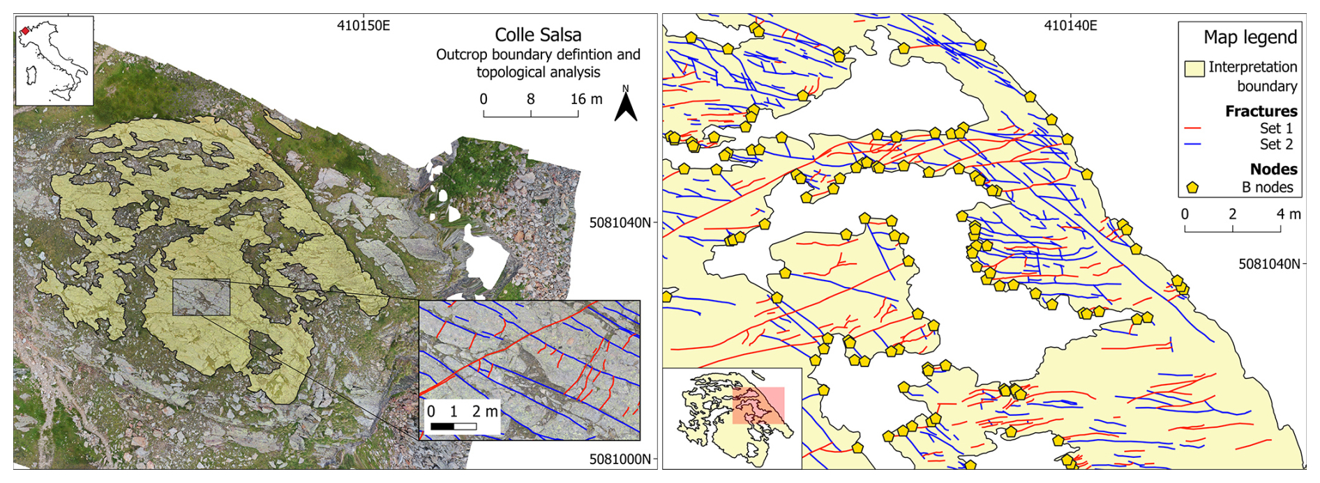
Figure 11 Overview maps of the second case study area. Pictured on the left is a general overview of the area with the boundary geometry overlaid on the orthophoto and a small sample of the digitized fracture sets. On the right is a subarea of the quarry with the boundary, fracture traces, and intersection nodes between the two (yellow pentagons).

The different estimated models are represented for both sets in Fig. 12. In both cases, the lognormal model better fits the data overall. Nonetheless, the fit of estimated models is visibly worse than in the first case study, particularly for Set 1 (Fig. 12a). The lognormal fit of Set 1 underestimates lengths between 0.34 and 1.5 m (about 50 % of the measures), while lengths above this value are generally overestimated. For the lognormal fit of Set 2 (Fig. 12b), there is a less relevant underestimation of the length values between 0.44 and 2.57 m (about 60 % of the measures) and a slight overestimation for longer length values. The distance values in Table 2 (ordered by ascending values of Akaike) confirm the lognormal as the most representative for both sets (see Fig. 13 for the summary plots of the best fit). For the other models, the mean rank value can be used to assign a final ranking. The mean ranks show that the gamma distribution is less representative than both the exponential and the Weibull (respectively the second- and third-most representative models).

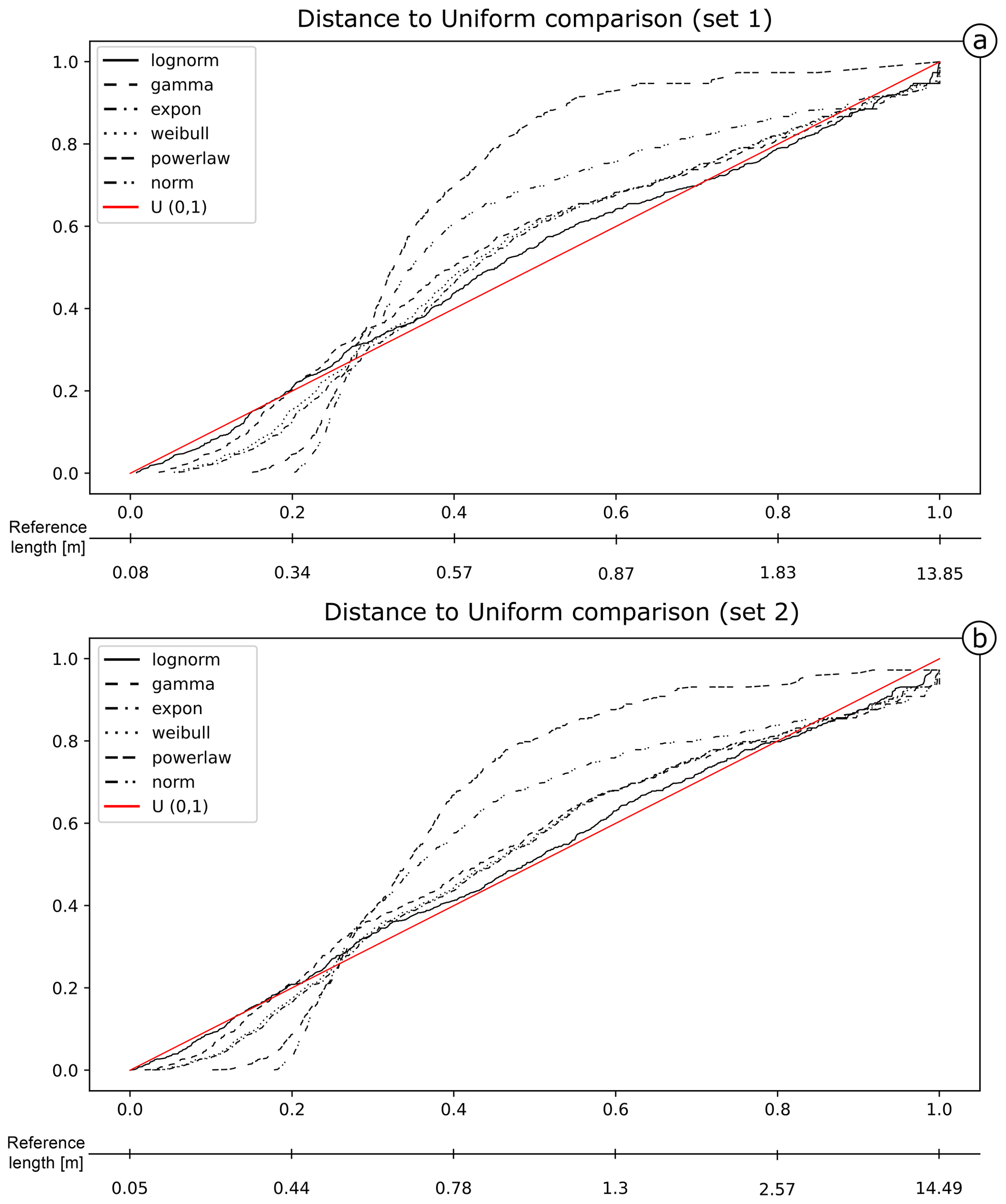
Figure 12 PIT visualization for the proposed length models is shown for Set 1 (a) and Set 2 (b) of the Colle Salza dataset. The red line represents the reference U(0,1); the closer a model's line is to this reference, the more representative the model. Among the models, the lognormal distribution demonstrates the closest fit to the reference line in both sets, although showing a worse fit to that observed in the first case study. Across both sets, all estimated models exhibit less linearity, with notable underestimation between 0.34 and 1.5 m in Set 1 (a) and between 0.44 and 2.57 m in Set 2 (b).

Table 2 Models' distance and rank tables for both Colle Salza sets. The closer to 0, the better. For this length dataset, the lognormal is the most representative of the data for all the different distances. Using the mean rank, the lognormal is followed by the exponential, Weibull, and gamma distributions. As with the first case study, the power-law and normal distributions are the least representative.

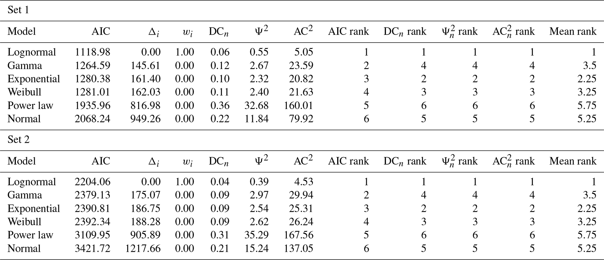
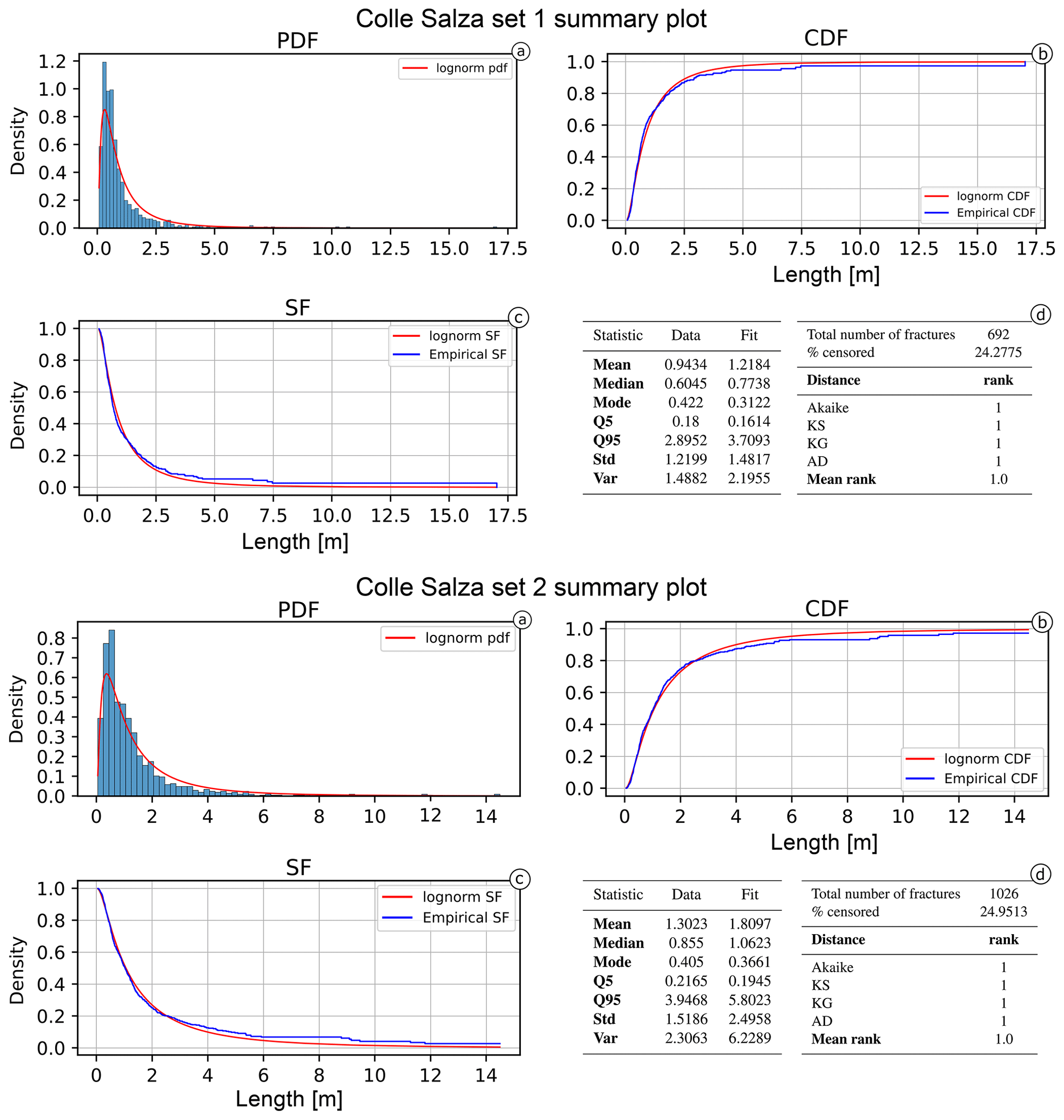
Figure 13 Summary of the best-fitting model for the Colle Salza dataset (Set 1 and 2). (a) The probability density function against the histogram of the dataset. (b) The cumulative distribution function and (c) the survival function against the empirical counterparts calculated with the Kaplan–Meier estimator. (d) The summary table of the main statistics for the data (e.g. sample mean, sample variance) and estimated model.

4.3 Third case study: spacing analysis

Survival analysis can also be used to analyse the spacing length distribution for each fracture set. Thus, the same workflow was applied to spacing measurements of both Set 1 and Set 2 of the Colle Salza dataset. It is worth noting that the censoring analysis is a secondary part of the analysis for spacing. Analysing the spatial arrangement of the fractures in the network (such as Marrett et al., 2018; Bistacchi et al., 2020) is of fundamental importance; however, we decided not to include this analysis and focus mainly on censoring to avoid increasing the length of an already dense text. Spacing is defined as the distance between two fractures of the same set, measured perpendicular to the average fracture plane attitude (Bistacchi et al., 2020, and references therein). Traditionally, this type of statistic is obtained in the field with scanline surveys, with properly oriented scanlines, or by applying the Terzaghi correction (Terzaghi, 1965). With DOMs, this procedure can easily be sped up with custom scripts, programmatically tracing a large number of parallel scanlines and thus increasing the number of spacing measurements (De Toffoli et al., 2021; Storti et al., 2022). However, this leads to a higher number of censored spacing measurements occurring at the outcrop boundary and where “holes” are present. As with standard lengths, the introduction of a boundary affects the actual estimation of the spacing by a degree depending on the outcrop's convexity (Fig. 14). Perfectly convex boundaries (Fig. 14b) will lead to minor censoring, affecting only the ends of the scanlines, while more realistic non-convex boundaries will increase the censoring percentage because the boundary will cross the same scanline at multiple points (Fig. 14c).

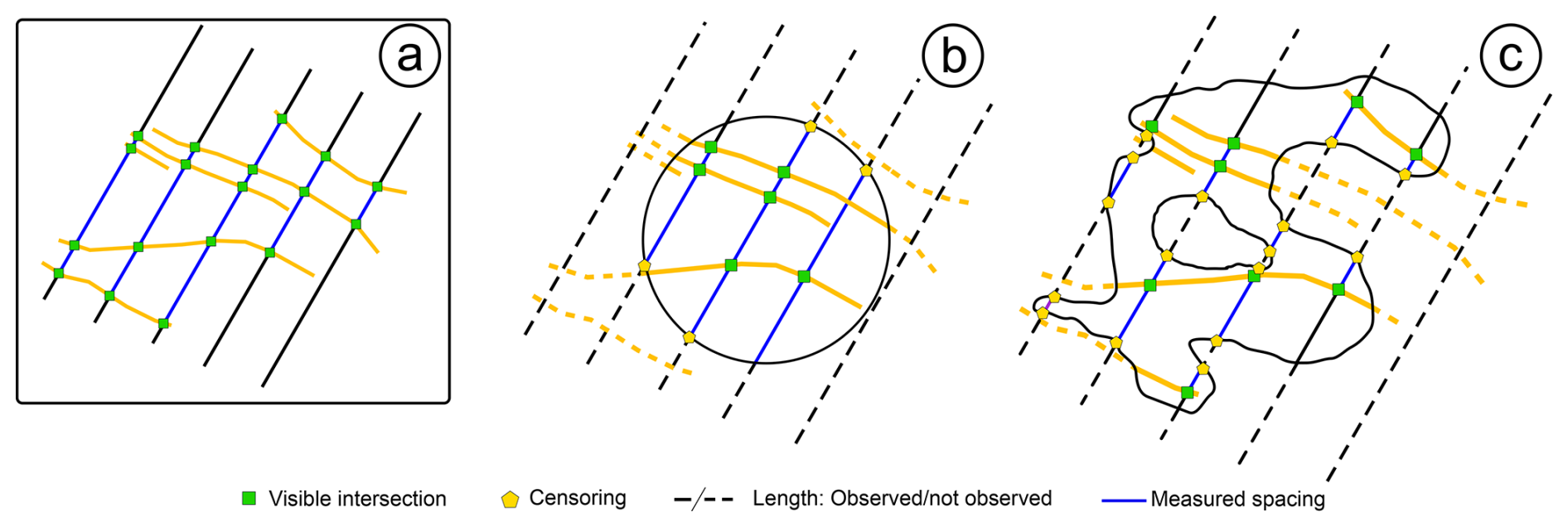
Figure 14 The effect of boundary geometry on censoring for spacing distribution modelling. (a) The ideal situation where no censoring occurs. The visible intersections between the scanline and the fracture are green, while the measured spacing segments are blue. (b) The effect of a perfectly convex boundary (i.e. a circle) on the estimation of censoring. For the “visible” scanlines, only the final segments are censored. (c) The effect of a complex boundary geometry. Here, the number of censoring measurements increases drastically, showing that censoring is no longer limited to the ends of the scanlines.

For the Colle Salza dataset, 1282 and 1119 spacing measurements were obtained for fracture sets 1 and 2 respectively (with 52.5 % and 36.5 % censoring). Figure 15 shows the distances of the different models for the obtained spacing values. In this case, for Set 1, an extreme underestimation of the lognormal model is present for values longer than 4 m (Fig. 15a), while, for the other proposed models, particularly the Weibull, the distances at the same values are smaller. This is also visible in the distance tables (Table 3). Although the Akaike distance for the lognormal model is the smallest, the difference from the other models (Δ_i) is not as big as in the other examples. Thus, the weight of evidence (w_i) is also not completely in favour of the lognormal model. The poor fit of the lognormal model is also confirmed by the other distances that rank the lognormal lower than the Weibull and gamma models (ranking first and second respectively). All these factors point to the fact that, in this case, the Weibull is the most representative model (see Fig. 16 for a summary representation of the best fit). Conversely, the lognormal model is clearly the most representative for Set 2 (Fig. 15b). The PIT plot shows a quite linear behaviour and all the calculated distances ranking first.

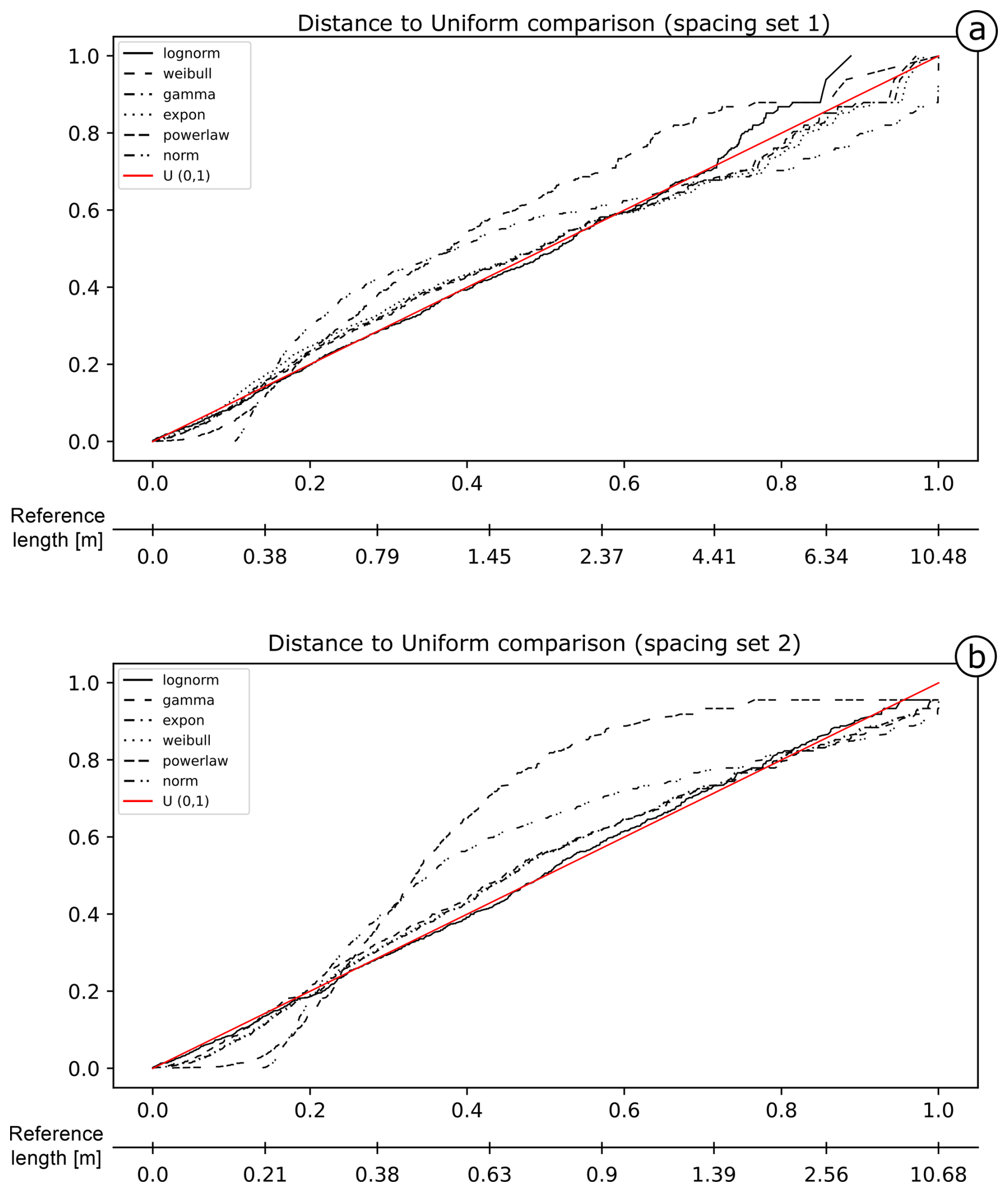
Figure 15 PIT visualization for the proposed length models is shown for Set 1 (a) and Set 2 (b) of the Colle Salza dataset. The red line represents the reference U(0,1); the closer a model's line is to this reference, the more representative the model. In contrast with the other case studies, the lognormal distribution demonstrates a marked underestimation for values longer than 4.4 m for the spacing of Set 1 (a). In this case, the closest fit is the Weibull. Conversely, for the spacing of Set 2 (b), the lognormal model is again the model closest to the reference line, performing similarly to the first case study.

Table 3 Models' distance and rank tables for the spacing calculated on both Colle Salza sets. The closer to 0, the better. For Set 1, the low performance of the lognormal in the estimation of longer values (Fig. 15a) is visible at all distances. Even if the Akaike distance calculated for the lognormal is the smallest, the difference from the other calculated values is not enough to completely justify the selection of this model. This is also shown in the other distances where the lognormal clearly underperforms. On the other hand, for Set 2, the lognormal model is the most representative for the spacing values for all the different distances.

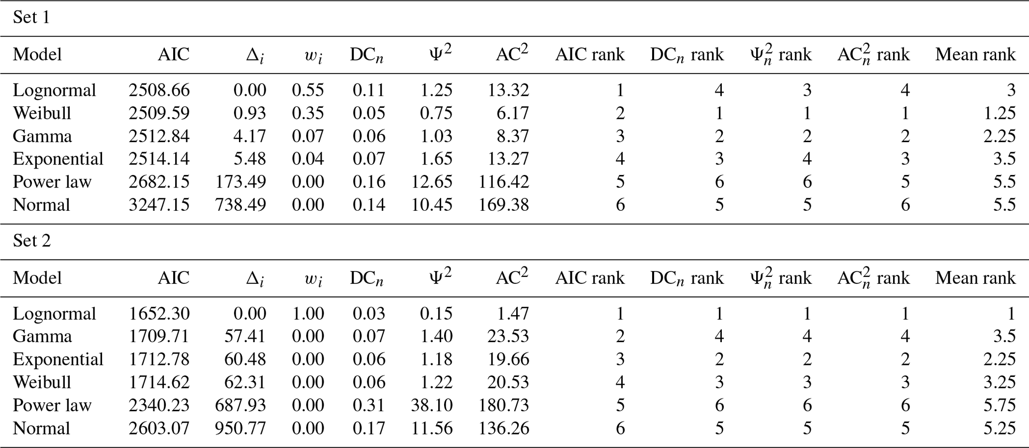
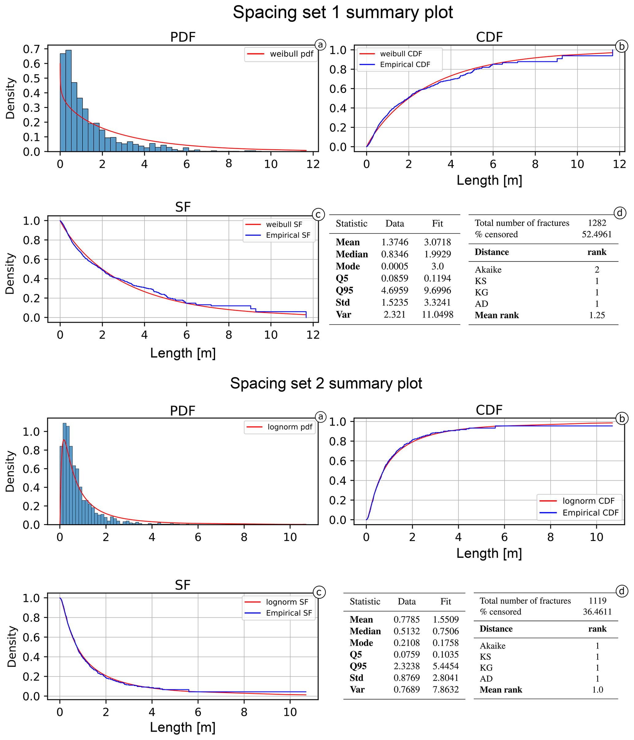
Figure 16 Summary of the best-fitting model for the spacing dataset (Set 1 and 2). (a) The probability density function against the histogram of the dataset. (b) The cumulative distribution function and (c) the survival function against the empirical counterparts calculated with the Kaplan–Meier estimator. (d) A summary table of the main statistics for the data (e.g. sample mean, sample variance) and estimated model. The spacing of Set 1 is the only case where the data are not lognormally distributed, and the frequency histogram reflects such a conclusion.

5 Discussion

With this work, we delineate a robust statistical framework to quantitatively analyse and statistically model fracture trace length and spacing. The statistical distributions are estimated using the entire length of fracture traces, following the original works of Baecher and Lanney (1978) and Baecher (1980) and not the length of branches as defined in Sanderson and Nixon (2015). Branches offer a useful topological abstraction of the network (making it possible to classify node intersections); however, they do not carry a real geological or physical meaning; thus a distribution obtained by fitting branch length will have a different meaning compared to one obtained from complete lengths. Furthermore, length can sometimes be affected by a subjective bias leading to an uncertainty as to which structure should be measured. For example, with segmented or en echelon fractures, do we measure the single segments or consider their cumulative sum? By approaching this problem with branches, a clear objective answer cannot be reached, while, by regarding a 2D lineament as a representation of the 3D geological structure, contextualized in the geological history of the outcrop, a more rational and informed decision can be made (i.e. Forstner and Laubach, 2022).

The first and crucial point of discussion is the objective of having a representative unbiased statistical model that is sufficiently likely to reproduce the observed length data. In particular, we want to stress that there is no real interest or practical reason and no theoretical possibility to find the real underlying distribution, while there is a strong necessity to fit specific simplified parametric models, useful for stochastic modelling applications (such as DFNs). Due to this, non-parametrical methods, such as those proposed by Mauldon et al. (2001), are unfit, since they are not linked to any model. Furthermore, having an unbiased statical model can also be extremely important for engineering applications. For example, at the end of the paper by Pahl (1981) it is stated that, in geomechanical application, it could be useful to know the longest trace likely to occur in a group of traces. With a parametric model, this can easily be estimated by checking the length values associated to a probability chosen, depending on the safety margin that is needed for the use case. Modern alternatives that use a simple implementation of MLE, such as FracPaQ (Healy et al., 2017), are a good step forward; however, the censoring bias is still present; thus the results are biased, always underestimating length. The approach proposed here provides for the middle ground that was missing. We have shown that it is possible to use survival analysis to model censored length datasets, and we have showcased a new approach in model selection via quantitative distances to rank and choose the most representative model from a pool of simple candidates that can be used in common modelling applications.

As stated, to use MLE for a given model, we assumed that, in geological applications, the only censoring mechanism present is random censoring. Both left and interval censoring, by definition, cannot happen because the event of interest coincides with the end of the fracture. Thus, for left censoring, fractures terminate outside the boundary and thus cannot be measured (this is analogous to a patient never entering the study because they are already dead). The same applies to interval censoring that could be erroneously identified when holes are present in the sampling area or when boundaries are concave. However, since the measured event is the end of the fracture, on the other side of the interruption no fractures should be present. In terms of classic survival analysis theory, this would compare to a patient's loss of follow-up in the study period, caused by voluntary or involuntary exit from the study group, thus classifying it again as right censoring (Leung et al., 1997).

To correctly classify censoring as random, we must assume independence between the censoring and length distribution. By “independence”, it is intended that the mechanisms behind the generation of a fracture-length distribution are different from the mechanisms that censor such lengths. The boundary, which represents censoring, is usually the product of secondary events that occur after fracture genesis (i.e. alteration, debris hiding part of the outcrop, vegetation, human activity). Thus, while it is often the case that such events are controlled by pre-existing structures, the physical processes that caused censoring are not the same ones that generated the fracture set and thus the original length distribution. This leads to an important implicit caveat where the measured lengths must be related only to the mechanism that we are interested in modelling, for example, lengths that are surely linked to tectonics and no other secondary events. Such discussion highlights that the assumption of independence is difficult to rigorously prove, since the true distribution of the length of fractures is not known (we only observe a set of complete and censored data). In some applications (Eppes et al., 2024), this assumption may not hold, and a more in-depth study may be required to prove the independence hypothesis before proceeding. Nonetheless, we believe that it can be safely assumed in geological applications when the appropriate field work and a posteriori analysis are carried out.

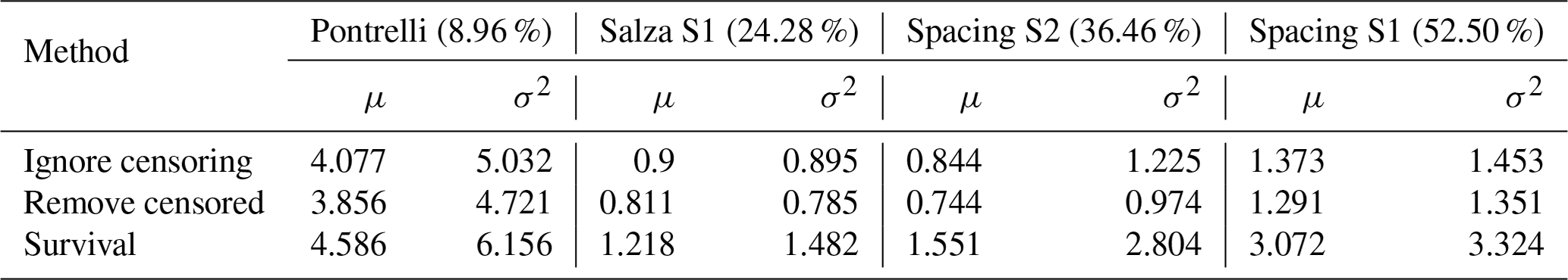
As a second point, we would like to discuss the relationship between the fraction of censored data and the uncertainty in the estimated statistical model. There is not much literature on this relationship, probably because, since traditional survival analysis is applied in the context of time, the time boundary can be expanded if necessary. For example, if a study shows a censoring rate that is deemed too high, the researcher could repeat the experiment and simply extend the study period to observe the event of interest. In our case, the spatial boundary usually cannot be expanded; thus knowing the effects of censoring on estimation is an important aspect. For example, it would be useful to know how censoring influences the estimations based on simplistic approaches described in Sect. 3, the censoring percentage value above which survival analysis must be used, or the value above which even survival analysis fails. Moreover, it can also be useful to estimate the precision of estimation with survival analysis, knowing the censoring percentage. The case studies discussed in this work show a censoring percentage ranging from 8.96 % (first case) to 52.50 % (third case) and effectively showcase the influence of censoring on the estimation. For each dataset, it is possible to use the best-fitting statistical model defined in the results and to use PIT plots to visualize the differences. The comparison with the circular scanline approaches was intentionally omitted because it cannot be compared in any way. Being a non-parametrical approach, cumulative frequencies cannot be compared, and comparing mean values without a variance is not informative. Figure 17 shows that, in all cases, the estimated model using survival analysis closely follows the reference uniform, while the other two approaches (i.e. ignoring censoring and removing censored data) always overestimate the cumulative frequency, diverging with a rate positively correlated with the censored fraction. This translates to an underestimation of a model's parameters proportional to the censoring percentage. This effect is due to the fact that measured lengths of censored fractures will always be shorter than their true lengths. Thus, by using the first simple approach, the dataset is essentially “polluted” by shorter fractures, thus always decreasing the measured mean. The second simple method will also lead to an underestimation of the mean because of the size bias. However, this second method can be less impacted by censoring. For example, if a fracture population has a very small standard deviation (i.e. almost all fractures have the same length) and/or fractures are occurring in an outcrop that is much bigger than the characteristic fracture length, then removing censored values would not have a great impact on the estimation. But, even if small, the underestimation will always be present. Overestimation of the mean length would be possible in these scenarios when we do not regard censoring as independent from the length distribution (for example, if only fractures shorter than a certain value are systematically censored). However, this would violate both the core underlying hypothesis of random censoring and standard geological experience; thus we do not deem it possible under these imposed limits. Furthermore, the model obtained by removing censored values is always the worst. This is because MLE is a consistent estimator that converges as the number of data increase; thus, by removing data, we are effectively hindering the estimator's precision (in the last case study, we removed 52 % of the data, i.e. 667 fractures). This effect is also visible when comparing the estimation of important distribution parameters such as mean (μ) and standard deviation (σ²). Table 4 compares the values of these parameters calculated with the different methods, showing a consistent underestimation of both the mean and the standard deviation, with a greater underestimation coming from the method that removes censored data.

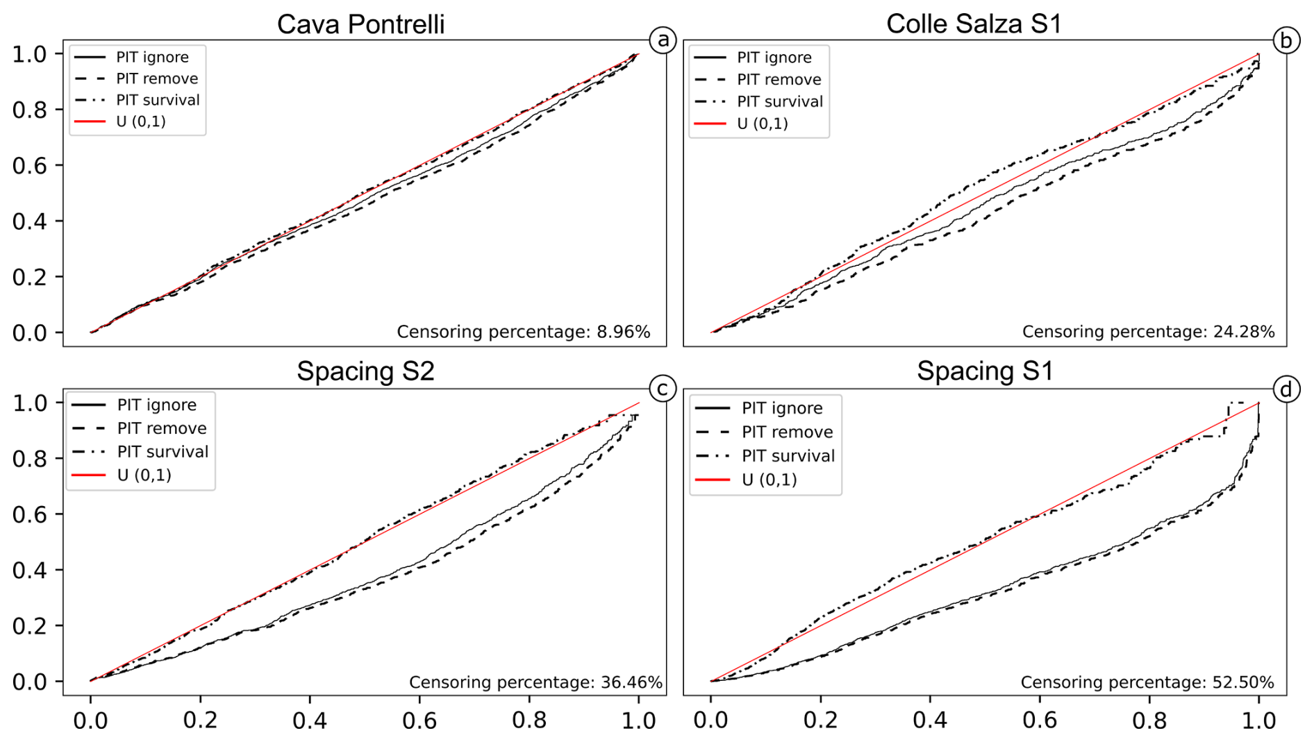
Figure 17 PIT visualization for the lognormal model estimated with three different approaches: ignoring censoring (full line), removing censored data (dashed line), and using a survival analysis approach (dashed–dotted line). The survival model follows the true model almost constantly (red line), while the other two approaches increasingly diverge on longer fractures with a rate depending on the censored fraction.

Table 4 Summary table comparing mean (μ) and standard deviation (σ²) values for increasing censoring fractions. The method ignoring censoring and the method removing censored data both underestimate the values, with the latter always showing a greater underestimation.

The outlined effect could be useful to predict what to expect from any survival analysis and shed some light on the exploration of the censoring mechanics that govern these types of datasets. Still, the comparison briefly discussed in this chapter is not rigorous enough to fully constrain this relationship. Even if we have a clear increase in the censoring percentage in the different datasets, the genetic factors, lithology, and censoring mechanics are completely different. Moreover, the number of measures in each case study are different and thus not statistically comparable. Because of these reasons, this behaviour should be isolated and modelled in controlled synthetic experiments to be carried out in the future. Nevertheless, we found that our preliminary results and the possible implications were too interesting not to be discussed.

As a third point, the readers that support and firmly believe in power-law distribution of length may be shocked by the results of this paper. In all the different case studies, the power-law distribution always ranked last or second to last together with the normal distribution. Power-law distributions theoretically describe many natural events, and, in our case, if fractures, for example, are self-similar, then the lengths could show a power-law distribution (Bonnet et al., 2001). However, it is shown that, in general, truncated power-law models better fit natural and realistic data; thus usually only the tails of the distribution follow a power law (Clauset et al., 2009). This means that, to properly fit a power law, it is necessary to estimate both the scaling parameter (α) and the minimum truncation value (x_min). Truncation is a constantly present bias caused by the resolution limits of the data source above or under which no data can be acquired (right and left truncation respectively). In our case, left truncation (i.e. x_min) is the most common type, and it is caused by the pixel resolution of the images under which fracture traces cannot be seen. Due to this limitation, for a constant-resolution scale, the modelled length distribution will always have an underestimation of the frequencies for the shorter lengths; thus usually only the tail of the distribution follows a power law. Adding to this bias is also the human error caused by countless different factors (one of which is the inevitable boredom of digitizing an outcrop). If the length distribution truly follows truncated power laws, then shorter fractures near the truncation limit would be much more frequent but harder to spot. Moreover, for some fracture systems, the smaller fractures are more prone to be mineral-filled and potentially less obvious features on images. This usually results in fractures that are left uninterpreted even if visible, thus leading to an increase in the real x_min value. Truncation bias and fitting power laws are a very active field of research still with no definitive solution (Clauset et al., 2009; Deluca and Corral, 2013); thus, the implementation, testing, and discussion of such solutions would lie outside this work. For the same reason, a proper estimation procedure could not be included, and the results obtained in this work relative to the power-law model must be taken with a grain of salt. Nonetheless, we still wanted to leave the estimation results and discussion of power laws to again show, as Healy et al. (2017) and Rizzo et al. (2017) did, how this model cannot be blindly applied to geological data without carrying out necessary important considerations.

Finally, censoring is one of many biases that influence the length measurements, and the presented work only treats this specific bias. Because of this, if other biases are present, they will also be carried out after the correction. Moreover, the underlying statistical model between different sets can be different; each fracture set has its own set of biases that influence measurements; and variation in the statistics can also occur within the same set, for example, in proximity of a fault or local changes in rheology. Because of all these reasons, grouping all entities in the same statistical model without any kind of consideration leads to inevitable misinterpretation of the statistics and provides a wrong statistical parametrization of the whole network; thus the analysis of a fractured rock system must be carried out in a homogeneous domain or different stationary domains must be defined before any further analysis is carried out (Bistacchi et al., 2020). By applying this divide-and-conquer approach, a more precise and robust characterization is assured because statistical models and inevitable biases related to different families will not mix. These observations further highlight the crucial importance of field data acquisition and geological reasoning to avoid blindly applying these methods to outcrops and making severe inferential errors.

6 Conclusions

In this paper, the effects of censoring bias on the estimation of statistical length models are delineated and discussed. In particular, we demonstrated that censoring bias leads to a general underestimation of any distribution. The typical approaches found in the literature are not suitable, and we have shown that using survival analysis is also the better way to treat censoring in length datasets. In particular, survival analysis offers a valid alternative to the popular circular scanline method. Firstly, survival analysis methods are based on the relationship between the event of interest and the censoring mechanism. Without any underlying geometrical assumptions (basis of the circular scanline method), this methodology is quite flexible and can easily be applied to any geological case study. Secondly, the parameters that are estimated with survival analysis are directly based on the measured length (i.e. the quantity that we want to model) and are always associated with a model; thus they have a higher statistical significance of the scanline method. Regarding the other parametrical methods (i.e. ignoring censoring and removing censored data), we have shown that the censoring percentage heavily influences the estimation quality. In particular, with only 8.96 % censoring, the two classical methods underestimate the mean and variance, and the increase in censoring percentage positively correlates with such underestimation. Also, survival analysis is visibly impacted by the increase in censoring; however, its output always remains stable around the natural model (i.e. the reference diagonal). Nonetheless, the influence of censoring percentage is not yet fully constrained, since, in this study, the visible variation is probably also given by different datasets, with different genetic factors. Thus, a more robust and in-depth analysis must be carried out to fully understand this relationship. The proposed combination of PIT plots and distance calculations demonstrates an effective approach to quantitatively rank a list of length distribution models. The workflow has the objective of comparing sensible (simple) models useful to practical applications (such as DFNs) and finding which one best represents the data. The theory and necessary tools to carry out a complete statistical characterization of a fracture network are included in the specifically developed FracAbility Python library (https://github.com/gecos-lab/FracAbility, last access: 8 September 2024), which encapsulates the necessary steps to carry out as easily and quickly as possible the workflow starting from input shapefiles. The methodology and library were successfully tested in three different use cases, the first having almost no censoring bias and the last with more than 50 % of the total measurements being censored. In all cases, except for the last, in which one of the two spacing distributions follows a Weibull distribution, the lognormal model was the most accurate, followed by either gamma, exponential, or Weibull.