Basic Earth Parameters from VLBI observations using Bayesian inversions in the time domain: updated insights of the Earth's interior

We present updated estimates of Basic Earth Parameters (BEP) from VLBI Celestial Pole Offset (CPO) time series spanning 1980-2025 using an ensemble Markov Chain Monte Carlo (MCMC) Bayesian inversion. Building upon Koot et al. (2008), we incorporate recent advances in ocean tidal modeling (Cheng and Bizouard, 2025) and update several aspects of the algorithm. Key improvements include: (1) implementation of a cubic spline representation for Free Core Nutation (FCN) amplitude variations, which significantly reduces multimodality in FCN-related parameter in MCMC sampling compared to a linear representation; (2) integration of updated Ocean Tidal Angular Momentum (OTAM) values from FES2014 ocean tidal atlas (Lyard et al., 2021), without the empirical 0.7 scaling factor previously applied in the construction of the last adopted nutation model MHB2000; and (3) utilization of five diverse CPO series from different analysis centers spanning up to 45 years of observations.

Our estimated mean values of the parameters show good consistency across different CPO series, with values of the Earth's dynamical ellipticity at the edge of the 1σ range of MHB2000 (Mathews et al., 2002; Buffett et al., 2002; Herring et al., 2002). Notable findings include a larger absolute value for the imaginary part of the core-mantle boundary (CMB) coupling constant (K^CMB), approaching the 2σ boundary of Mathews et al. (2002), which may reflect contributions from other coupling mechanisms in addition to electromagnetic coupling, including possible topographic coupling through “form drag” effect caused by wave interactions with irregular boundaries (Rekier et al., 2025). The real part of the Inner Core Boundary (ICB) coupling constant (K^ICB) is approximately half the MHB2000 value, potentially indicating the need to revisit hydrostatic assumptions for the inner core given recent seismic evidence of viscous deformation (Wang et al., 2024; Vidale et al., 2025). Compliance estimates suggest that frequency extrapolation methods from seismic to nutation bands may be considered unchanged in the mantle, but should be revised at the ICB. The enhanced FCN free-mode modeling captures amplitude variations that differ from empirical models, particularly after 2000, although the physical interpretation of these differences requires further investigation.

The systematic discrepancies across multiple parameters suggest that current nutation theory needs substantial updates to incorporate more realistic models of core-mantle coupling and inner-core–outer-core coupling.

1 Introduction

Accurate knowledge of Earth orientation variations is essential for astronomy, geophysics, and space navigation applications. The Earth's rotation varies both in orientation and angular velocity because of its non-spherical shape, non-rigid and inhomogeneous interior, and the gravitational forces from celestial bodies, especially the Sun and the Moon. Developing theoretical models accurate enough to match current observational precision serves the dual purpose of enabling precise Earth orientation predictions and constraining the dynamical processes and the internal structure of Earth's deep interior (Dehant and Mathews, 2007, 2015; Gross, 2015).

The Earth's rotation is described by a set of Earth Orientation Parameters (EOP): nutation corrections, also called Celestial Pole Offsets (CPO) with respect to a conventional model (dX,dY), pole coordinates in the Earth-attached reference frame (x_p, y_p), and UT1–UTC or the Length of Day (LOD) (Petit and Luzum, 2010). The current conventional model of the precession-nutation is the IAU 2003/2000A model, also called MHB2000 (Mathews et al., 2002), adopted by the International Union of Geodesy and Geophysics (IUGG) and the International Astronomical Union (IAU) in 2003 and 2000, respectively. Among these rotational variations, nutation is uniquely suited for probing Earth's internal structure because the external gravitational forcing can be calculated with high precision, allowing observed deviations to be attributed to properties of Earth's interior (Mathews et al., 1991, 2002; Dehant and Mathews, 2015).

These variations are continuously monitored by geodetic techniques such as Very Long Baseline Interferometry (VLBI), Global Navigation Satellite System (GNSS), Satellite Laser Ranging (SLR), and Doppler Orbitography and Radiopositioning Integrated by Satellite (DORIS). These observations are organized by dedicated international services in an operational way to maintain the International Celestial Reference Frame (ICRF) and the International Terrestrial Reference Frame (ITRF).

VLBI uses radio telescopes separated by large distances on the Earth's surface to form baselines to observe selected quasars simultaneously, measuring the differences in the reception time of the wavefront at the two stations at both ends of the baseline. Among these techniques, VLBI is the only one that uses extragalactic radio sources as reference points in the sky, which enables it to determine the orientation of the Earth in space with respect to a long-term stable reference frame and thus to obtain the Earth's orientation variations, i.e., precession associated with the trend and nutations associated with the periodic part. Geodetic VLBI observations started in the 1970s, and their precision has improved significantly in the late 1980s (Carter et al., 1984). The precision and network infrastructure have been continuously improved since then.

The modeling of the Earth's nutation starts from the computation of the variations caused by gravitational forces from the Sun, the Moon and the planets of the solar system acting on a rigid Earth with dynamical flattening determined by the luni-solar precession constant (Dehant and Capitaine, 1996; Dehant and Mathews, 2015). The latest rigid Earth nutation model is REN2000 (Souchay and Kinoshita, 1996, 1997; Souchay et al., 1999). Then, a transfer function is used to determine the amplitudes of these periodic motions (Dehant and Mathews, 2015), taking into account the existence of the fluid outer core (FOC) and the solid inner core (SIC), coupling effects at the core-mantle boundary (CMB) and the inner core boundary (ICB), the anelasticity of the Earth, and the angular momenta and loading of the external fluid layers composed of the oceans and the atmosphere (Koot and de Viron, 2011). Parameters related to these characteristics of the real Earth are called the Basic Earth Parameters (BEP) (Koot et al., 2008; Mathews et al., 2002).

The authors of the current conventional nutation model, MHB2000 (Mathews et al., 2002), estimated some of the BEPs from VLBI observations spanning from 1980–1999. They deduced a nutation spectrum from these observations, and then estimated the BEPs with least-squares fitting. Koot et al. (2008) estimated the same set of BEPs from VLBI observations in the time domain using Bayesian inversion, estimating BEPs directly from the CPO time series observed by VLBI. Their results are mostly consistent with those of MHB2000, except for the imaginary part of the coupling constant at the ICB (ℑ(K^ICB)), which is twice in absolute value of that of MHB2000. Zhu et al. (2017) performed estimations with both methods with VLBI observations up to 2015. They also got larger values for the imaginary part of K^ICB, confirming the results of Koot et al. (2008). Since the last adopted nutation model in 2000, we have almost 25 more years of data with better quality (45 years of VLBI observation in total). In addition, global ocean models (Lyard et al., 2021) and consequently the ocean tidal effects on nutation have been updated (Cheng and Bizouard, 2025). It is time to renew the estimations of BEPs with the objective to provide new insights into the characteristics of the Earth's interior and interactions between the different parts of it.

In this work, we build upon the foundation established by Koot et al. (2008), employing an ensemble Markov Chain Monte Carlo (MCMC) scheme to perform Bayesian inversion of BEPs using VLBI CPO time series spanning from 1980–2025 (with slight variations for each series). Our analysis also benefits from the latest evaluation of ocean tidal effects on nutations (Cheng and Bizouard, 2025), where the Ocean Tidal Angular Momentum (OTAM) (Lyard and Alain, personal communication, used in Cheng and Bizouard, 2025) is derived from the FES2014 ocean tidal atlas (Lyard et al., 2021).

In the following sections, we first present the basic structure of the inversion algorithm, focusing on FCN modeling and OTAM updates, followed by results from different CPO series and recommendations for BEP values, including the new insights they provide into the Earth's deep interior.

2 Methods and model updates

The Bayesian inversion algorithm for BEP estimation used in this work was developed by Koot et al. (2008) based on the nutation theory of MHB2000 (Mathews et al., 1991, 2002). We provide a brief description of the structure of the algorithm here for the sake of clarity and interpretation of the results. Readers interested in more details are invited to consult the original papers.

Bayesian inversion is an algorithm based on Bayes' theorem that determines the probability distributions of parameter values using a posterior function derived from a given model (in this case, the nutation model with the set of BEPs to be estimated) and observations. Unlike traditional inversion algorithms based on least-squares fitting, Bayesian inversion does not require linearization of the relationships between observables and the parameters to be estimated. We updated the sampling algorithm from a single Metropolis–Hastings sampler (Metropolis et al., 1953; Hastings, 1970) to an ensemble (multi-walker) Markov Chain Monte Carlo (MCMC) scheme implemented with the Python package “emcee” (Foreman-Mackey et al., 2013). We set the number of walkers to five times the number of estimated parameters. This approach enables a more efficient and complete stochastic sampling of the probability landscape around the maximum of the posterior probability density function.

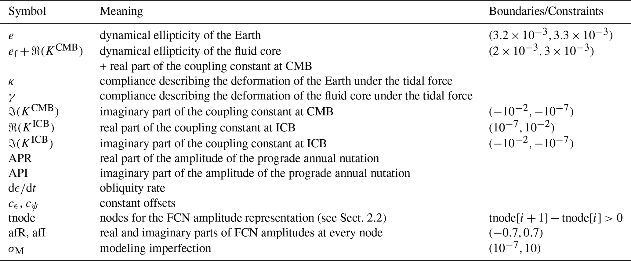
2.1 The posterior probability density function and free parameters

The posterior function is established as follows (Koot et al., 2008):

$$\begin{array}{}\text{(1)}& \begin{array}{rl}{\displaystyle }& {\displaystyle }p(\mathit{\theta },{\mathit{\sigma }}_{\mathrm{M}}|\mathrm{\Delta }{\mathit{\psi }}_{t_i},\mathrm{\Delta }{\mathit{ϵ}}_{t_i})\propto \mathit{\pi }({\mathit{\sigma }}_{\mathrm{M}}\left)\mathit{\pi }\right(\mathit{\theta })\\ {\displaystyle }& {\displaystyle }\times {\prod }_{i=\mathrm{0}}^N{\displaystyle \frac{\mathrm{1}}{\sqrt{({\mathit{\sigma }}_{\mathit{\psi }}\sin {\mathit{ϵ}}_{\mathrm{0}}{)}^{\mathrm{2}}+{\mathit{\sigma }}_{\mathrm{M}}^{\mathrm{2}}}\times \sqrt{{\mathit{\sigma }}_{\mathit{ϵ}}^{\mathrm{2}}+{\mathit{\sigma }}_{\mathrm{M}}^{\mathrm{2}}}}}\\ {\displaystyle }& {\displaystyle }\times \exp \left\{-{\sum }_{i=\mathrm{0}}^N\left[{\displaystyle \frac{\mathrm{1}}{\mathrm{2}}}{\displaystyle \frac{(\mathrm{\Delta }{\mathit{\psi }}_{t_i}-\mathit{\delta }\mathit{\psi }(\mathit{\theta },t_i\left){)}^{\mathrm{2}}\right(\sin {\mathit{ϵ}}_{\mathrm{0}}{)}^{\mathrm{2}}}{({\mathit{\sigma }}_{\mathit{\psi }}\sin {\mathit{ϵ}}_{\mathrm{0}}{)}^{\mathrm{2}}+{\mathit{\sigma }}_{\mathrm{M}}^{\mathrm{2}}}}\right]\right.\\ {\displaystyle }& {\displaystyle }-\left.{\sum }_{i=\mathrm{0}}^N\left[{\displaystyle \frac{\mathrm{1}}{\mathrm{2}}}{\displaystyle \frac{{\left(\mathrm{\Delta }{\mathit{ϵ}}_{t_i}-\mathrm{\Delta }\mathit{ϵ}(\mathit{\theta },t_i)\right)}^{\mathrm{2}}}{{\mathit{\sigma }}_{\mathit{ϵ}}^{\mathrm{2}}+{\mathit{\sigma }}_{\mathrm{M}}^{\mathrm{2}}}}\right]\right\},\end{array}\end{array}$$

where θ is one of the free parameters listed in Table 1, $\mathrm{\Delta }{\mathit{\psi }}_{t_i}$ and $\mathrm{\Delta }{\mathit{ϵ}}_{t_i}$ are the nutation in longitude and obliquity at time t_i, ϵ₀ is the obliquity at J2000, and σ_M, σ_ψ, and σ_ϵ are the uncertainties in the modeling, the nutation in longitude, and the nutation in obliquity, respectively. π(σ_M) and π(θ) are priors, assumed to have a uniform probability, within the ranges given in Table 1. For simplicity of implementation, the log-posterior is used, i.e., the logarithm of the posterior probability distribution used in Bayesian inference. It can be written as

$$\begin{array}{}\text{(2)}& \begin{array}{rl}{\displaystyle }& {\displaystyle }{\log }_{e}p\simeq -{\sum }_{i=\mathrm{0}}^N\left[{\displaystyle \frac{(\mathrm{\Delta }{\mathit{\psi }}^{O-C}\sin {\mathit{ϵ}}_{\mathrm{0}}{)}^{\mathrm{2}}}{{\mathit{\sigma }}_{\mathit{\psi }}^{\mathrm{2}}}}+{\displaystyle \frac{(\mathrm{\Delta }{\mathit{ϵ}}^{O-C}{)}^{\mathrm{2}}}{{\mathit{\sigma }}_{\mathit{ϵ}}^{\mathrm{2}}}}\right]\\ {\displaystyle }& {\displaystyle }-{\sum }_{i=\mathrm{0}}^N{\log }_e\sqrt{({\mathit{\sigma }}_{\mathit{\psi }}\sin {\mathit{ϵ}}_{\mathrm{0}}{)}^{\mathrm{2}}+{\mathit{\sigma }}_{\mathrm{M}}^{\mathrm{2}}}\\ {\displaystyle }& {\displaystyle }-{\sum }_{i=\mathrm{0}}^N{\log }_e\sqrt{{\mathit{\sigma }}_{\mathit{ϵ}}^{\mathrm{2}}+{\mathit{\sigma }}_{\mathrm{M}}^{\mathrm{2}}}-{\log }_e\left|\mathrm{\Im }\right(K^{\text{CMB}}\left)\right|\\ {\displaystyle }& {\displaystyle }-{\log }_e\left|\mathrm{\Im }\right(K^{\text{ICB}}\left)\right|-{\log }_e\left|\mathrm{\Re }\right(K^{\text{ICB}}\left)\right|-{\log }_e\left|{\mathit{\sigma }}_{\mathrm{M}}\right|\end{array}\end{array}$$

where $\mathrm{\Delta }{\mathit{\psi }}^{O-C}=\mathrm{\Delta }{\mathit{\psi }}_{t_i}-\mathit{\delta }\mathit{\psi }(\mathit{\theta },t_i)$, and similarly for Δϵ.

Since the algorithm operates in the time domain, nutation corrections are computed for each epoch in the chosen VLBI series. For each frequency term in the rigid-Earth nutation model REN2000 (Souchay et al., 1999), the algorithm reads the corresponding amplitudes and calculates the transfer functions at those frequencies. These transfer functions, which incorporate the Basic Earth Parameters (BEPs), are then applied to the rigid-Earth nutation amplitudes to obtain the “real” Earth nutation amplitudes. The calculated nutation value at each epoch is formed by summing these frequency-domain contributions.

To compute the posterior function, the algorithm adds nutation values from the MHB2000 model to the Celestial Pole Offset (CPO) series, and then subtracts the calculated values from the current parameter set in the MCMC run. These residuals are used to evaluate the posterior probability function (see Eq. 28 of Koot et al., 2008). Since the amplitude of the Free Core Nutation (FCN) varies with poorly understood excitations, several parameters are introduced to model these variations. An additional parameter accounts for model imperfections (see Sect. 5.3 in Koot et al., 2008). All free parameters in this setup are listed in Table 1.

Table 1 Free parameters in the Bayesian inversion setup.

2.2 Free Core Nutation modeling

The Free Core Nutation (FCN) is a rotational eigenmode of an Earth with a deformable solid mantle and a fluid core, and it can only be observed if it is excited. This eigenmode exists due to the presence of a fluid, flattened, and deformable core. It is retrograde (opposite to the direction of the Earth's rotation) and has a period of approximately 430 d in space. The frequency of the FCN is close to diurnal in an Earth-fixed frame, so it is also called the Near Diurnal Free Wobble (NDFW). It was discovered in the 1980s thanks to the improved precision of geodetic observations enabled by the development of VLBI. The community generally attributes the excitation of this free mode to oceanic and atmospheric loading which have nearby frequencies (Kiani Shahvandi et al., 2024), or to jerks within the core, i.e. sudden/abrupt changes in the second time derivative in the Earth's magnetic field observed at the surface (Cui et al., 2020), but the nature of this excitation remains unclear, which is why the FCN eigenmode amplitude and phase cannot be predicted and must be estimated from nutation corrections obtained by VLBI observations.

The authors of the MHB2000 model estimated the FCN eigenmode amplitude and phase using a 4 year sliding window from VLBI observations, while fixing the FCN eigenperiod. They then removed the resulting time-variable contribution before using the observed VLBI residuals to estimate the BEPs by performing the inversion in the frequency domain. Meanwhile, the fixed frequency of the FCN (in cycle per mean solar day) used in the eigenmode determination is intrinsically related to some of the BEPs as:

$$\begin{array}{}\text{(3)}& \begin{array}{rl}{\displaystyle }{f}_{\text{FCN}}=& {\displaystyle }-\left(\mathrm{1}+{\displaystyle \frac{A_{\mathrm{f}}}{A_{\mathrm{m}}}}\right)\\ {\displaystyle }& {\displaystyle }\times \left[e_{\mathrm{f}}+\mathrm{\Re }\left(K^{\text{CMB}}\right)-\mathit{\beta }+{\displaystyle \frac{A_{\mathrm{s}}}{A_{\mathrm{f}}}}\mathrm{\Re }\left(K^{\text{CMB}}\right)\right].\end{array}\end{array}$$

where A_m, A_f and A_s are the moments of inertia in the equatorial plane of the Earth's mantle, the FOC, and the SIC, respectively. Therefore, such a sequential approach leaves the nutation and FCN eigenmode modeling to some extent inconsistent.

Koot et al. (2008) performed the inversion in the time domain, which allows FCN modeling to be integrated into the estimation of the BEPs. We build on their work and explore the integration of more sophisticated modeling of the FCN eigenmode within this estimation framework.

The conventional empirical FCN model is constructed by fitting a harmonic oscillation with a period of −430.21 d to CPO series observed by VLBI, using a sliding-window approach to capture temporal variations in amplitude. The window length is chosen to be 7 years to demodulate the FCN from the retrograde annual oscillation, and it slides every half year (Lambert, 2007) (see https://ivsopar.obspm.fr/fcn/, last access: 10 April 2025). We take this as a reference to compare with the amplitude variations captured by our parameterizations.

To account for the time variability of the FCN amplitude, we model it using piece-wise functions. Considering the length of the CPO time series and the computation time, and after testing the influence of the number of notes on the other BEPs, the number of nodes is set to 12.

2.2.1 Piece-wise linear modeling of FCN amplitude

We first use a piece-wise linear model inherited from Koot et al. (2008). In addition, since the larger quantity of data (longer VLBI CPO time series) supports improved sampling capability, we allow the locations of the nodes (time points separating different pieces of the piece-wise linear function) to vary freely, except the first and the last ones that are set to be at the beginning and the end of the VLBI CPO time series used in the inversion. Experiments show that this method suffers from convergence issues for FCN-related parameters. This is easy to understand because multiple different arrangements of node positions may explain the data equally well, which inevitably leads to different plausible configurations during the MCMC sampling process. We address this issue by applying a clustering algorithm (k-mean) to the output samples of an initial run, in which the node positions are free to adjust, selecting the “most frequent” combination of node positions. The MCMC is then rerun with these fixed node positions.

2.2.2 Cubic-spline modeling of FCN amplitude

In addition, since the amplitude variations between nodes is clearly not linear in time, we implement a cubic spline to replace the linear function in the inversion process. This approach allows us to capture the continuous and non-linear changes in the FCN amplitude over time, while still allowing the node positions to vary together with the BEPs. The results show that this modification significantly reduces the multimodality of the FCN-related parameters during MCMC sampling, to the extent that clustering and rerunning are no longer necessary. We discuss these results in more detail in the dedicated section.

2.3 OTAM from FES2014

Ocean tidal effects account for a significant portion of the nutation perturbations due to the non-rigidity of the Earth. Their contributions are particularly important for the determination of the rotational normal modes of the Earth in the presence of the fluid outer core and the solid inner core. The oceanic tidal contributions to nutation can be calculated from Ocean Tidal Angular Momentum (OTAM) estimated from a global ocean tidal model. The OTAM is composed of two parts: the “matter” term arising from ocean height (load), and the “motion” term arising from ocean currents. In practice, one computes only the “principal terms” (see Table 3 of Cheng and Bizouard (2025), and Table 3 of Chao et al. (1996) for MHB2000). Contributions to nutation from the other tidal terms are interpolated by means of an ocean admittance (see Mathews et al. (2002) (denoted as MHB2000 hereafter) or Cheng and Bizouard (2025) (denoted as BCFES2014 hereafter) for more details). In this interpolation process, MHB2000 applied a constant scaling factor of 0.7 to the admittances to account for inaccuracies in ocean tidal maps. They pointed out that this inaccuracy arises mainly from the calculation of the current angular momentum, whose large contributions substantially come from small but deep oceanic regions. This number was determined by examining the effects of different constant scaling factors on their fit results. However, it is not clear whether it was applied only to the current (motion) term or to both current (motion) and load (mass) terms. Cheng and Bizouard (2025) calculated the effects of major tidal terms on nutation separately and reported significant differences compared to those of the MHB2000 nutation model (see Table 2). These differences arise mainly from updated ocean tide maps, while the contribution from differences in the transfer function is not significant. For the interpolated terms, Cheng and Bizouard (2025) found good agreement among tidal amplitudes estimated from different series of CPO with respect to MHB2000. The observed residual amplitudes are about 30 % of the values predicted by BCFES2014. This suggests that the 0.7 scaling factor applied in the MHB2000 model may no longer be necessary.

Table 2 Differences of amplitudes of typical ocean tidal terms (BCFES2014-MHB2000) from Cheng and Bizouard (2025).

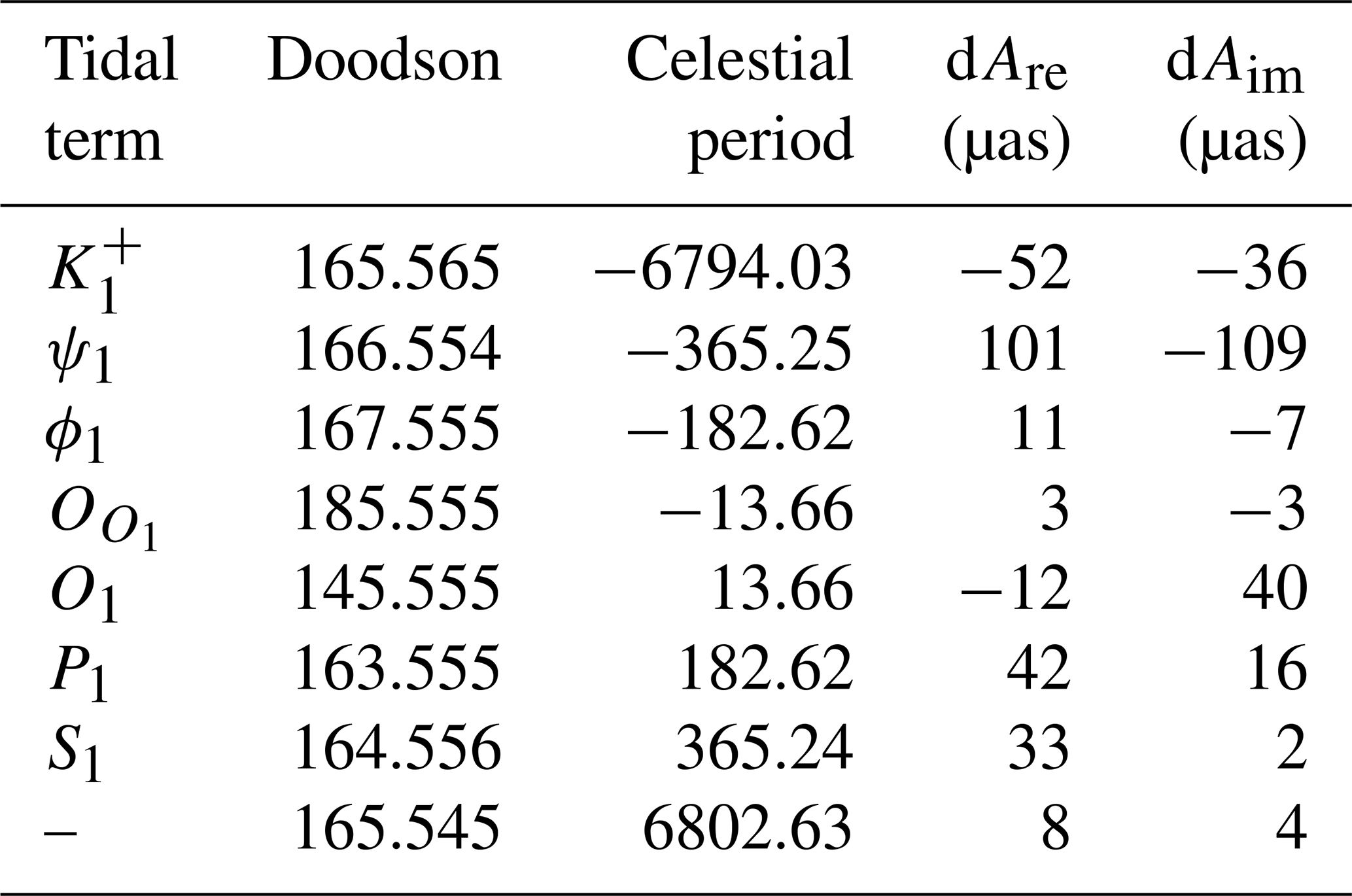
Table 3 Matter (ma) and motion (mo) terms of the equatorial ocean angular momentum raised by the ocean tides according to FES2014 model (F. H. Lyard and D. J. Allain, personal communication, 2020). Amplitude ($h_x^{\mathit{\sigma }},h_y^{\mathit{\sigma }}$) in unit of 10²⁴ kg m² s⁻¹, phase $({\mathit{\varphi }}_x^{\mathit{\sigma }},{\mathit{\varphi }}_y^{\mathit{\sigma }})$ in degrees.

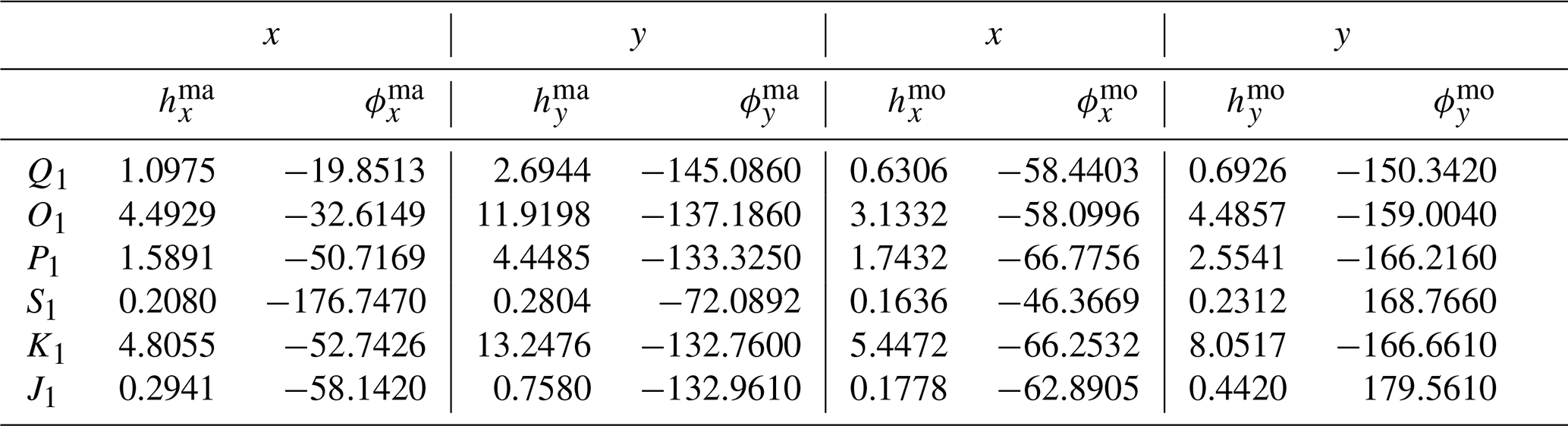
In this study, we update the OTAM values using those calculated from the FES2014 ocean tidal atlas (Lyard and Alain, personal communication, used in Cheng and Bizouard, 2025), and retain the same dynamics equations and ocean admittance interpolation without any scaling factor. Note that compared to MHB2000, the J₁ tide is now also included among the main waves derived from the ocean tide map and contributes to the determination of the interpolation function.

3 Results and discussions

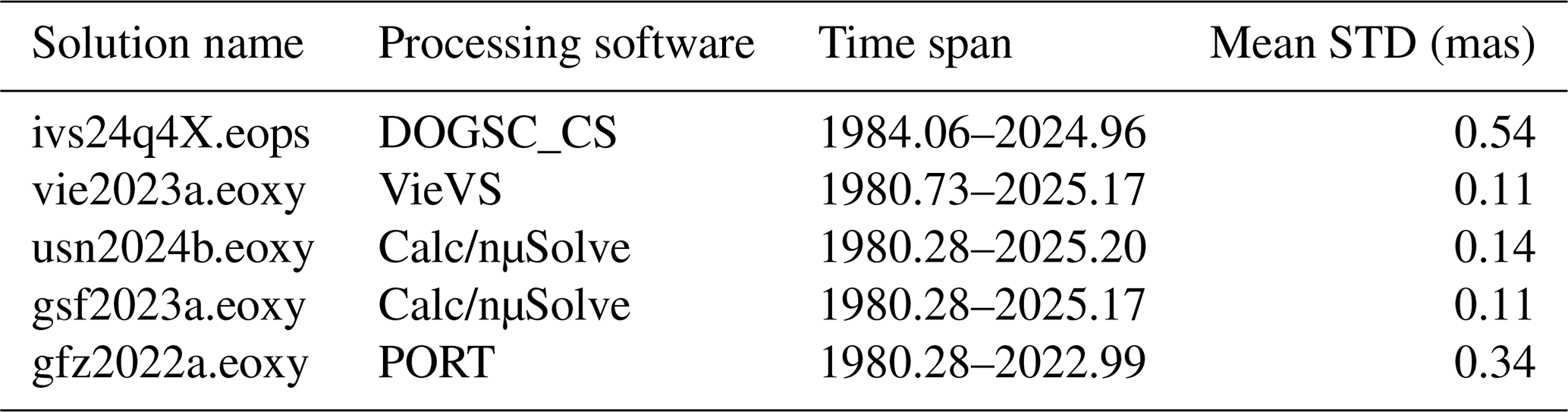
We base our estimations on the most up-to-date CPO series from different analysis centers that use different software for post-processing. They are listed in Table 4. They are provided by the International VLBI Service for Geodesy and Astrometry (IVS; Nothnagel et al., 2017) and archived at NASA's Crustal Dynamics Data Information System (CDDIS; Noll, 2010). Note that the ivs24q4X series is a solution-level combination of series from different analysis centers adopted by the International VLBI Service (IVS) combination center.

Table 4 CPO series used in this study.

3.1 Methodological improvements and their impact on BEP estimation

We demonstrate the effects of our methodological enhancements using the usn2024b CPO series as a representative example. Two improvements are examined: the implementation of updated Ocean Tidal Angular Momentum (OTAM) corrections and the adoption of piece-wise cubic spline modeling for FCN amplitude variations.

We replace the OTAM values from Chao et al. (1996), used for the ocean contributions in MHB2000, with those derived from the FES2014 ocean tidal atlas (Lyard et al., 2021), removing the empirical 0.7 scaling factor applied in MHB2000. The updated OTAM values show significant differences from the original model, particularly for major tidal terms (see Table 2). These changes propagate through the oceanic corrections and directly impact the estimated BEPs, especially the compliances (κ and γ) and coupling constants (K^CMB and K^ICB), as shown in Fig. 1. Note that in our solution using OTAM values from Chao et al. (1996), the scale factor of 0.7 is not applied.

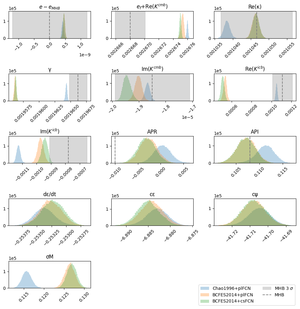
Figure 1 Distributions of BEPs from usn2024b, with different OTAM values (from Chao et al., 1996) and “BCFES2014” (Cheng and Bizouard, 2025) and different modeling of FCN amplitudes (“pl” for piece-wise linear and “cs” for piece-wise cubic spline), compared with MHB2000 values (black lines) and 3σ ranges (grey areas). e_MHB2000=0.0032845479.

We can see in Fig. 3 that the use of cubic splines affects the choice of node positions and better captures the amplitude variations of the FCN eigenmode. It is generally very close to the empirical model (Lambert, 2007), but some differences are observed, especially after 2000. Figure 4 shows FCN amplitudes from all series using cubic spline modeling with 12 nodes. They are generally in agreement (within 3σ) with the empirical model of Lambert (2007).

The differences between piece-wise linear and cubic spline modeling of FCN amplitudes can be seen in the coupling constants, not only in the one that is directly related to the FCN frequency (K^CMB), but also in K^ICB, which is related to the inner core coupling and the frequency of the Free Inner Core Nutation (FICN).

Finally, Fig. 2 shows the distributions of BEPs from all series using cubic spline modeling with 12 nodes, and the corresponding estimated values and their standard deviations are listed in Table 5. We will discuss them in the following section.

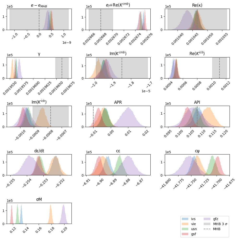
Figure 2 Distributions of BEPs from all series, compared with MHB2000 values (black lines) and 3σ ranges (grey areas). FCN amplitudes in these cases are modeled as piece-wise cubic splines with 12 nodes (see Fig. 4). e_MHB2000=0.0032845479.

Koot et al. (2008)

Table 5 Estimated BEPs with standard deviation from all used CPO series, applying BCFES2014 OTAM and using cubic spline with 12 nodes for FCN modeling. Values from MHB2000 and Koot et al. (2008) are listed in the last two columns for comparison. Also see histograms in Fig. 2. Uncertainties are given at 1σ values (calculated as the standard deviation of the samples).

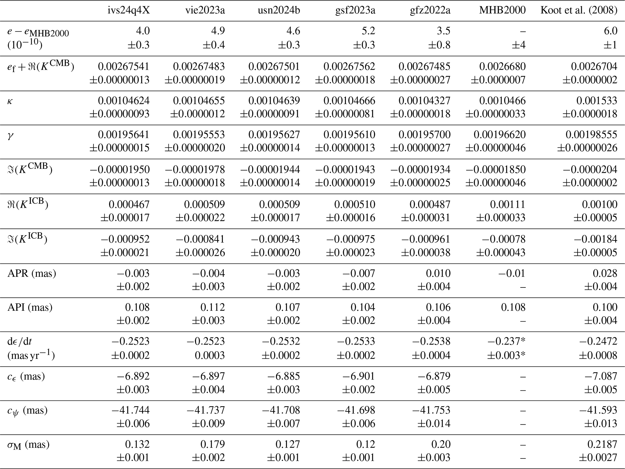
* Note that the MHB2000 value of $\mathrm{d}\mathit{ϵ}/\mathrm{d}\mathit{\psi }$ comes from Herring et al. (2002) where the obliquity rate ($\mathrm{d}\mathit{ϵ}/\mathrm{d}\mathit{\psi }$) and constant offsets (c_ϵ and c_ψ) are estimated with amplitudes of 21 nutation terms, while the values of constant offsets are not given. e_MHB2000=0.0032845479.

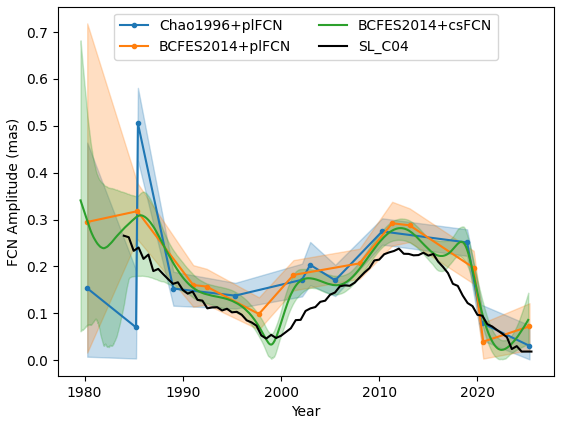
Figure 3 Amplitude variations of the Free Core Nutation (FCN) from usn2024b, with different OTAM values (from Chao et al., 1996) and “BCFES2014” (Cheng and Bizouard, 2025) and different modeling of FCN amplitudes (“pl” for piece-wise linear and “cs” for piece-wise cubic spline), compared with the empirical model fitted with a sliding window (Lambert, 2007) (in black). Solid lines represent the median of the posterior ensemble, and the shaded band shows the 99.7 % credible interval (equivalent to ±3σ for a Gaussian distribution), obtained by evaluating the spline (or piecewise linear) interpolation over under-sampled posterior draws and computing the 0.15th–99.85th percentiles at each time point.

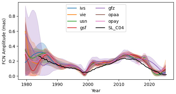
Figure 4 Amplitude variations of the Free Core Nutation (FCN) from all series, compared with the empirical model (in black). In these cases, the variations are modeled as piece-wise cubic splines with 12 nodes for each series. Solid lines represent the median of the posterior ensemble, and the shaded band shows the 99.7 % credible interval (equivalent to ±3σ for a Gaussian distribution), obtained by evaluating the spline interpolation over thinned posterior samples and computing the 0.15th–99.85th percentiles at each time point.

3.2 Geophysical interpretations

3.2.1 Dynamical ellipticities and the core-mantle coupling

The dynamical ellipticities e estimated from all series are in good agreement, lying at the edge of the 1σ range of the MHB2000 value. This parameter is related to the precession rate, which is correlated with the 18.6 year nutation. The CPO series used here cover about two periods of the 18.6 year nutation.

The dynamical ellipticity of the FOC (e_f), the real part of the coupling constant at the CMB (ℜ(K^CMB)), and the compliance β cannot be estimated independently, as they appear as a linear combination in the equation describing the nutations (e.g., Eq. 29 in Mathews et al., 1991). The estimate of $e_{\mathrm{f}}+\mathrm{\Re }\left(K^{\text{CMB}}\right)-\mathit{\beta }$ is significantly larger than the MHB2000 value. The compliance β is fixed to the value calculated from the Preliminary Reference Earth Model (PREM, Dziewonski and Anderson, 1981) by Mathews et al. (2002), which includes the effects of mantle anelasticity), since it is the parameter for which the theoretical value has the smallest uncertainty (Koot et al., 2008). Any departure of the real part of β from this value can be considered included in this term. A reevaluation and numerical separation of these correlated parameters will require careful theoretical consideration.

More notably, the estimated imaginary part of K^CMB has a larger absolute value than MHB2000. This increase was already noted by Koot et al. (2008), but it becomes more pronounced in the present work as the value approaches the 2σ boundary of MHB2000 value. Following the relationship illustrated in Fig. 1 of Mathews et al. (2002) (see also Fig. 2 of Buffett et al., 2002), for a conductive layer of 200 kilometers with a high conductivity of $\mathrm{5}\times {\mathrm{10}}^{\mathrm{5}}{\text{S m}}^{-\mathrm{1}}$ (equal to that of the core) and a large skin depth (penetration of the time-varying magnetic field into the lower mantle), the matching with K^CMB derived from VLBI observation would require an RMS radial magnetic field of approximately 0.75 mT through electromagnetic coupling alone. Such a field strength would require unrealistically high and uniform conductivity throughout the lower mantle (Lobanov et al., 2021), which is likely too optimistic given that the skin depth is of the order of a few hundred meters (Buffett et al., 2002). Recent work by Rekier et al. (2025) proposes an alternative mechanism involving topographic coupling through form drag and internal wave excitation at the CMB, which could explain the observed dissipation without requiring unrealistically high lower-mantle conductivity or magnetic field strength. The larger ℑ(K^CMB) values we observe may therefore reflect contributions from multiple coupling mechanisms rather than purely electromagnetic effects.

This makes it difficult to interpret our estimate of e_f, since the contribution of electromagnetic coupling to ℜ(K^CMB) is uncertain. We can nevertheless provide constraints under different scenarios. Mathews et al. (1991) estimated that e_f exceeds the hydrostatic value (e_f[hydrostatic]=0.002548) by about 3.8 %, corresponding to an increase of the core equatorial radius of 370 m. From our estimates, if ℜ(K^CMB)=0, e_f increases by about 4.9 % relative to the hydrostatic value. If we attribute all observed ℑ(K^CMB) to electromagnetic coupling, leading to $\mathrm{\Re }\left(K^{\text{CMB}}\right)\approx \mathrm{2.5}\times {\mathrm{10}}^{-\mathrm{5}}$, then e_f increases about 4.0 % comparing to the hydrostatic value. In both cases, this implies a non-hydrostatic contribution corresponding to an increase in the core equatorial radius between about 370 and 500 m.

3.2.2 The inner core

Our estimation of ℜ(K^ICB) appears to be almost half of the MHB2000 value. This decrease can already be seen in Koot et al. (2008), but is again much more noticeable in this work. This parameter is related to the Free Inner Core Nutation (FICN) frequency (in cycle per mean solar day), as explained in Koot et al. (2008) and Mathews et al. (2002):

$$\begin{array}{}\text{(4)}& {\mathit{\sigma }}_{\text{FICN}}\simeq -\mathrm{1}+{\mathit{\alpha }}_{\mathrm{2}}{e}_{\mathrm{s}}+\mathit{\nu }-K^{\text{ICB}}\end{array}$$

where α₂=0.8294 is a constant defined in Mathews et al. (1991) and related to properties of the Earth's interior such as the density jump at the CMB, and e_s=0.00242 is the dynamical ellipticity of the SIC. Both values are computed from PREM. K^ICB is the complex coupling constant at the ICB and ν is the compliance related to deformation of the ICB.

Similar to ℜ(K^CMB), ℜ(K^ICB) appears as a linear combination with α₂e_s +ν. In our inversion setup, the values of e_s and α₂ are fixed to those calculated by Mathews et al. (2002) from PREM, under the assumption that the inner core boundary corresponds to a surface of hydrostatic equilibrium, which was supported by studies in the late 1990 s, estimating dynamic topographies associated with mass anomalies in the inner core and in the mantle to be below 100 m at ICB (Defraigne et al., 1996). Note that the compliance ν is also fixed to the value calculated from PREM for the same reason as β. Considering electromagnetic coupling only, our value would require a magnetic field at the ICB lower than in MHB2000, and thus closer to geodynamo results (between 10 and 40 Gauss [0.1–0.4 T], Aubert, 2013). Recent studies by Wang et al. (2024) and Vidale et al. (2025) have revealed, from seismic data, possible viscous deformation at the inner core boundary (ICB) occurring on timescales of years. The hydrostatic assumption for the inner core in nutation computations could thus be revised. In addition, the density jump at the ICB could also be reconsidered in light of possible evidence for a mushy zone at the ICB (Tian and Wen, 2017).

Moreover, our estimation of the imaginary part of K^ICB is slightly larger in absolute value compared to MHB2000, which is, in a way, contradictory to the result for the real part, considering the relationship shown in Fig. 2 of Mathews et al. (2002) (see also Fig. 2 of Buffett et al., 2002) for electromagnetic coupling at the ICB.

3.2.3 Compliances

Compliances describe the deformability of the Earth or of specific regions of its interior, under a given forcing. The two compliances that are important to consider in our free parameter set are κ, which characterizes the deformability of the whole Earth under tidal forcing, and γ, which characterizes the deformability of the fluid core under tidal forcing.

These compliances reflect the anelasticity of Earth's interior, which is frequency dependent. Their values are initially derived from PREM (Dziewonski and Anderson, 1981), whose rheological parameters were constrained by high-frequency seismic data (with periods from several seconds to one hour) and subsequently extrapolated to the nutation band (diurnal frequencies) through a power-law scaling with frequency to account for anelasticity. The exponent of this power-law scaling, however, is poorly constrained.

In MHB2000, the compliance values estimated from VLBI data were consistent with the theoretical values obtained through this extrapolation. Our results break this consistency: our estimate of κ remains in complete agreement with MHB2000, but our estimate of γ is significantly smaller. Since both compliances are corrected from their elastic values through the same anelastic extrapolation procedure, a shift in γ without a corresponding shift in κ cannot be explained by simply adjusting the power-law exponent. This points to a limitation in the current anelastic correction framework, or in the PREM model from which the elastic compliances are derived, and calls for careful systematic revision.

3.2.4 Corrections to the prograde annual terms

The atmosphere contributes to nutation mainly at the prograde and retrograde annual, semi-annual, and ter-annual frequencies. There is also a contribution to the retrograde annual nutation due to the resonance effect with the FCN. Evaluating these effects using atmospheric angular momentum (AAM) data remains non-trivial, as it requires data with a high sampling rate to capture quasi-diurnal effects in a frame tied to the Earth. The largest effect occurs at the prograde annual frequency. Therefore, a prograde annual term is included among the estimated parameters to account for this atmospheric effect as it is the most important contribution (Yseboodt et al., 2002). The results of our estimations of this term differ by about 20 µas among different solutions from various IVS analysis centers. It should be noted that this prograde annual term is empirical and will absorb not only the atmospheric contribution but also any other signals appearing in VLBI observations as prograde annual oscillations, which are typically associated with the Earth's revolution around the Sun and the resulting annual temperature variations.

Two CPO series are generated using Calc/nµSolve to test the effect of different mapping functions of the tropospheric delay in VLBI data processing. The considered mapping functions are VMF1 (re3data.org, 2020) and NMF (Niell, 1996). The resulting differences appear primarily in the prograde annual term at the level of 2 µas, which corresponds to the uncertainty of this parameter in individual data series. The differences in K^CMB and K^ICB are not significant.

3.2.5 Additional parameters

We have considered the same set of additional parameters that are adjusted at the same time with the geophysical parameters as those in Koot et al. (2008): the obliquity rate $\mathrm{d}\mathit{ϵ}/\mathrm{d}t$, constant offsets c_ψ and c_ϵ, and the modeling uncertainty σ_M. Their presence in MHB2000 is not obvious, but they were actually evaluated by Herring et al. (2002) before the final BEP estimations for MHB2000 by Mathews et al. (2002).

The obliquity rate $\mathrm{d}\mathit{ϵ}/\mathrm{d}t$ was estimated together with 21 nutation frequencies by Herring et al. (2002). Their result is also included in Table 5. Herring et al. (2002) also estimated the secular obliquity change with nutation amplitudes fixed to MHB2000 values, where they found $\mathrm{d}\mathit{ϵ}/\mathrm{d}t=-\mathrm{0.252}\pm \mathrm{0.003}\mathrm{mas}{\mathrm{yr}}^{-\mathrm{1}}$, which is closer to our result. Note that the FCN is also estimated in both cases with its time-varying amplitude represented as piece-wise linear functions, with 6 and 10 nodes for time series spanning about 20 years. However, their results for the constant offsets c_ψ and c_ϵ are not given.

The parameter σ_M, introduced by Koot et al. (2008), incorporates both the modeling error and a constant correction to the standard deviation of the data (see Eq. 28 in Koot et al., 2008). Standard deviations are used to represent the uncertainties of CPO estimates from VLBI observations, but they are usually smaller than the true uncertainties. With σ_M, this possible underestimation of CPO uncertainties is taken into account. It thus partially serves the same purpose as the parameter introduced by Herring et al. (2002) to correct data errors.

4 Concluding remarks

This study presents an updated estimation of Basic Earth Parameters from VLBI observations by Bayesian inversion, incorporating 25 additional years of higher-quality data compared to the conventional nutation model MHB2000 (Mathews et al., 2002; Herring et al., 2002; Buffett et al., 2002). Our enhanced methodology, incorporating ensemble MCMC sampling, cubic spline FCN amplitude modeling, and updated OTAM corrections, provides robust parameter estimates with improved precision compared to Mathews et al. (2002) and Koot et al. (2008).

The consistency of results across five CPO series from different analysis centers using different post-processing software validates our approach and strengthens confidence in the estimated values. These estimations provide new geophysical insights, including evidence for additional coupling mechanisms at the core-mantle boundary, challenge the current inner and outer core models, and point to the need for revised frequency scaling laws for Earth's anelastic response. The larger ℑ(K^CMB) values we observe are consistent with recent theoretical work by Rekier et al. (2025) on topographic coupling from form-drag theory, suggesting that electromagnetic coupling alone cannot fully explain the observed dissipation at the CMB.

Our FCN free-mode modeling reveals amplitude variations that show systematic differences from Lambert (2007) empirical model after 2000, highlighting remaining uncertainties in our understanding of FCN excitation processes. The halved ℜ(K^ICB) value (compared those in MHB2000 and Koot et al., 2008), combined with recent seismic evidence for inner core deformation on annual timescales or for a mushy zone at the ICB, suggest that hydrostatic equilibrium assumptions for the shape of the ICB in nutation theory may require revision.

The updated BEP values provide refined constraints on Earth's deep interior structure and dynamics, but the persistent discrepancies between observations and theory across multiple parameters indicate that fundamental aspects of the nutation model may need revision. The larger coupling constants, altered compliances, and FCN amplitude differences collectively suggest that our current theoretical framework, while substantially improved since MHB2000 in different respects, needs to be revised for the physics considered inside the Earth as well as for consistency, as already highlighted by Ferrándiz et al. (2020).

The results of this work will inform future Earth rotation modeling and contribute to our understanding of core-mantle and inner core boundary processes. The methodology presented here provides a robust computational framework for parameter estimation that can accommodate more sophisticated theoretical models. As our understanding of Earth's interior dynamics continues to evolve, future work should prioritize the development of a unified nutation theory that integrates recent advances in core-mantle coupling mechanisms, outer core fluid dynamics, and anelastic response models. Such a consistent theoretical framework is essential to reconcile the systematic parameter differences revealed by this expanded VLBI dataset and to fully exploit the growing precision of geodetic observations for Earth science applications.