New insights on the fault structure of Bedretto geothermal testbed and the associated seismicity based on active seismic crosshole tomography

Fat ray travel time tomography was used to obtain reliable high-resolution subsurface images in the geothermal testbed of the Bedretto Underground Laboratory for Geosciences and Geoenergies (BedrettoLab). The aim of the research was to better understand the relationship between structural features and the seismicity induced by hydraulic stimulation tests. Eight boreholes were used to provide a large data set comprising 41 881 manually picked first breaks. Our results demonstrate that the fat ray approach offers improved image quality compared to traditional ray-based methods. The 3D model was further validated using ground-truth information from wireline logs and geological observations. We successfully imaged a major fault zone (MFZ) that exhibits a complex structure including considerable heterogeneity. Relocation of passive seismic events generated during hydraulic stimulations indicates that the 3D velocity model has only a minor influence on hypocentral parameters. However, comparing a selection of well-constrained seismic events with the velocity structures revealed a remarkable spatial correlation. Most events occurred in regions of intermediate and slightly decreased seismic velocities, thereby avoiding both high- and very low-velocity zones. Based on small-scale laboratory studies, we speculate that these observations can be explained by the presence of stress gradients in the intermediate-velocity zones.

1 Introduction

Energy production from sustainable resources is a key challenge of this century. Geothermal energy is recognized as a viable option. In particular, so-called “enhanced geothermal systems” (EGS) may have the potential to produce affordable electrical energy (e.g. Olasolo et al., 2016; Hirschberg et al., 2015). Key challenges include establishing sustainable flow rates, while controlling the associated induced seismicity (Zang et al., 2024). Examples of EGS projects that had to be stopped due to high seismicity include Basel (Edwards et al., 2015) and Pohang (Ellsworth et al., 2019). These problems are closely linked with the often poorly known fracture network of the reservoir. Therefore, several initiatives have been established to better characterize relevant host rock structures with near-field observations and well-monitored stimulation experiments (Amann et al., 2018; Obermann et al., 2024; Kneafsey et al., 2025). Seismic studies offer powerful tools for imaging key structures, such as permeable fracture zones, which are the main targets of EGS investigations. They can be applied during an initial characterization phase or during the stimulation phase. Generally, these studies are either passive or active seismic techniques. Passive techniques do not require actively fired seismic sources. Instead, information contained in ambient noise is exploited (e.g., Obermann and Hillers, 2019) or recordings of the induced seismicity are analyzed. For example, Charléty et al. (2006) conducted a 4D tomographic study using induced seismicity at the Soultz-sous-Forêts Hot Dry Rock site in France; that is, temporal 3D seismic velocity changes were computed. Active seismic methods can be subdivided into reflection and refraction imaging and transmission tomography. Reflection and refraction imaging can be carried out either from the surface, or surface-to-borehole configurations – also referred as vertical seismic profiling (VSP). In geothermal applications, VSP is particularly popular. For example, Nakata et al. (2023) used VSP data for reflection imaging of faults and fractures at the geothermal test site FORGE, Utah, U.S.A. It is also possible to combine induced seismicity methods with reflection imaging. Block et al. (1994) applied a joint hypocenter-velocity inversion using induced seismicity from Hot Dry Rock (HDR) experiments at Los Alamos National Laboratory, New Mexico to gain a 3D velocity model. Nakagome et al. (1998) used a seismic reflection survey together with vertical seismic profiling (VSP) to image the fractured reservoir in the Kakkonda geothermal field (Japan). Place et al. (2011) employed induced seismicity and VSP data to map fractures in Soultz-Sous-Fôrets (France). Transmission tomography primarily makes use of direct, diving or refracted waves traveling from sources to receivers. It can be either applied from the surface (e.g., Zelt and Barton, 1998; Lanz et al., 1998; Heincke et al., 2006), or between boreholes (e.g., Pratt and Worthington, 1988; Maurer and Green, 1997). Here, the travel times of the first arriving waves are exploited to establish 2D or 3D distributions of the seismic velocities. Alternatively, the first break amplitudes can be used to compute attenuation models (e.g., Holliger et al., 2001). All these studies provided useful information for a better understanding of the subsurface structures. Since seismic waves travel in a heterogeneous medium along complicated wave paths, 2D tomographic investigations suffer from inherent limitations, resulting from the assumption that the wave paths lie exclusively within the tomographic (2D) plane. Therefore, 3D investigations should be carried out when complex subsurface structures are expected. This can be achieved quite easily with surface-based investigations, because the sources and receivers can be well distributed over the earth’s surface, resulting in good seismic ray coverage of the structures of interest, given that acquisition offset is large enough. In the case of crosshole investigations, this is often a problem because there are rarely enough boreholes available to allow a good ray coverage of the subsurface region of interest. Therefore, 3D crosshole tomography experiments are very rare, which is unfortunate because they can potentially offer very relevant and unique subsurface information. The problem of poor ray coverage can be, at least partially, alleviated with the concept of fat rays, where it is assumed that seismic waves are not traveling along infinitesimally thin rays, but within “fat rays”, whose thickness is governed by the dominant frequencies of the seismic waves (e.g. Woodward, 1992). The initial concepts provided by Woodward (1992) have allowed fat ray approaches to be implemented for local earthquake tomography (Husen and Kissling, 2001) and active seismic experiments (Jordi et al., 2016). We have applied these concepts for the host rock characterization at the BedrettoLab (Ma et al., 2022; Plenkers et al., 2022). As discussed in more detail in Sect. 2, the BedrettoLab is a unique research environment that includes a geothermal testbed, which mimics a realistic reservoir structure in crystalline rocks. For example, it includes important structures, such as a major fault zone (MFZ). In total, nine boreholes were drilled within the geothermal testbed, out of which eight were available for active seismic measurements. This offered exciting opportunities for testing the benefits and limitations of 3D travel time tomography. As described in this contribution, several active seismic crosshole measurements were carried out, and they were analyzed using the fat ray tomography approach. The primary aim of our study is to image important geological structures and to better understand the relationship between these structural features and the seismicity, induced by various hydraulic stimulation experiments, within the geothermal testbed. We start with a description of the BedrettoLab, the embedded geothermal testbed, and briefly summarize key results from previous investigations in the BedrettoLab. We then present our data set, followed by a short description of the methodology employed to establish the 3D velocity models. After the presentation of the tomographic results, we perform a joint interpretation with geological and geophysical add-on data sets that were also acquired at our test site. In particular, we discuss the spatial correlation between passive seismic events and the velocity structures found.

2 Site description

The Bedretto Underground Laboratory for Geosciences and Geoenergies (BULGG or BedrettoLab), operated by ETH Zurich, is located in the central Swiss Alps (Ticino) in a 5.2 km long side tunnel of the Furka railway tunnel (Fig. 1a). The BedrettoLab is a unique research facility that provides optimal conditions for conducting experimental research to understand the responses of deep underground structures during hydraulic stimulations. With dimensions at the hectometer scale (hundreds of meters extension), the BedrettoLab closes the gap between the decameter laboratory scale (tens of meters extension, e.g., Grimsel test site; Gischig et al., 2020) and the reservoir scale (hundreds of meters to kilometers; Amann et al., 2018).

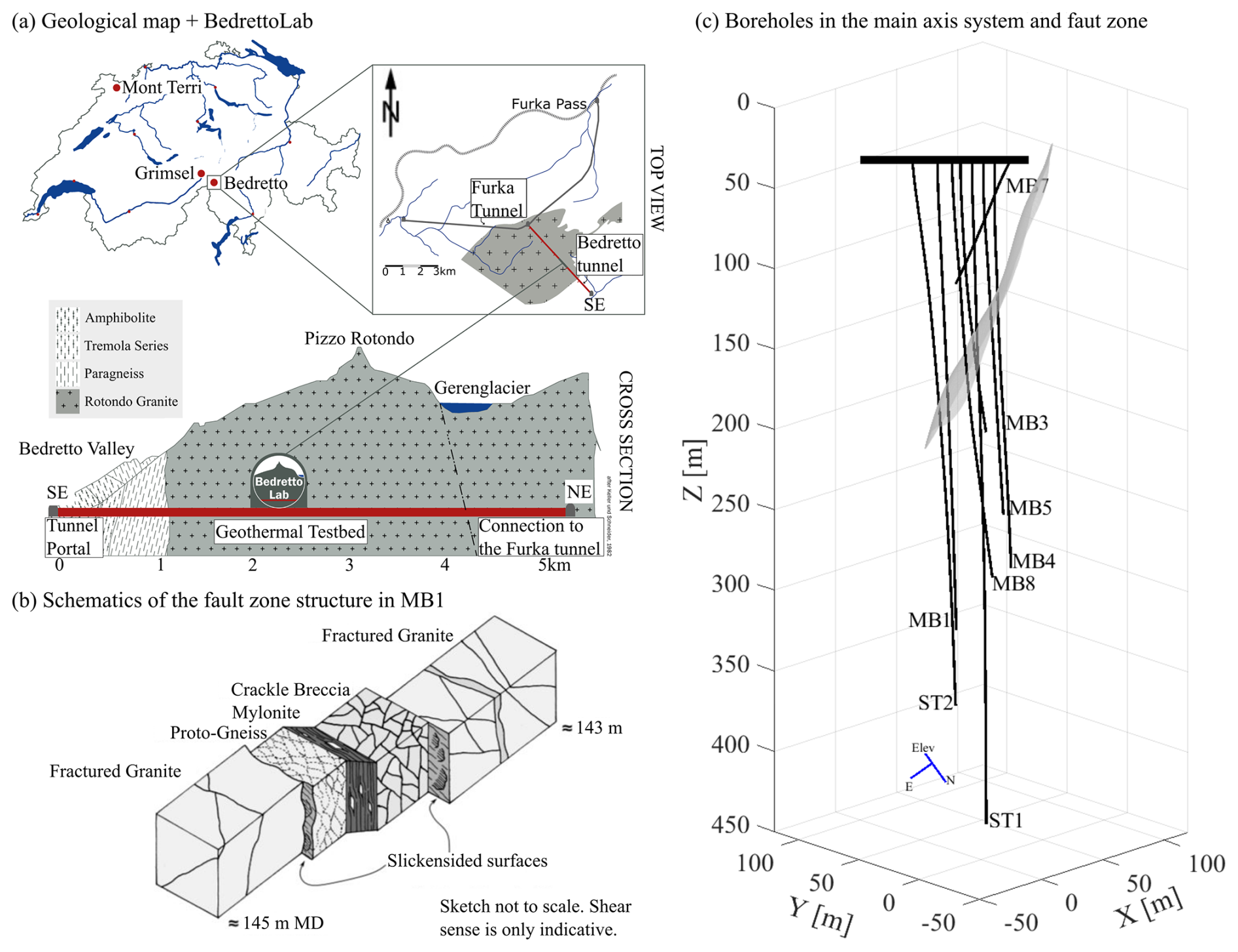
Figure 1 (a) Location and geological map of the BedrettoLab (see Rast et al., 2022; Ceccato et al., 2024). (b) Schematics of the Major Fault Zone (MFZ), observed in borehole MB1. The MFZ is found at depth of 143 and 145 m in this borehole. Fractured Granites surround Porto-Gneiss, Myolonite and Crackle Breccia (figure adjusted from Ma et al., 2022). (c) Boreholes drilled into the Geothermal Testbed, including six monitoring boreholes (MB1, MB3-MB5, MB7, MB8), one stimulation (ST1) and one extraction (ST2) borehole. Here, the boreholes are shown in the tomography coordinate system used in this paper. The blue arrows show the orientation of the original Bedretto coordinate system with Easting, Northing and Elevation, as used in panel (a). Additionally, panel (c) depicts the 3D structure of the MFZ (gray surface) as derived by Escallon et al. (2024).

The BedrettoLab host rock is composed mainly of granites, which are referred to as the Rotondo Granite. Its intrusion into the Gotthard Massif took place during the late Variscan orogeny (Sergeev et al., 1995). In general, the Rotondo Granite is homogeneous, that is, it generally exhibits isotropic structures of the physical properties, but in some places, weak signs of metamorphism are observed (Labhart T, 2005; Lützenkirchen and Loew, 2011). This may have slightly altered the isotropic structures (see also Fig. 1b). Behnen et al. (2025) identified weak signs of anisotropy near the geothermal testbed, but for the sake of simplicity, we assume an isotropic velocity structure for this study. According to the World Stress Map (Heidbach et al., 2018), the main horizontal compressive stresses are oriented in NW-SE direction, but Bröker et al. (2024a) showed that within the BedrettoLab, the orientation of the stress field can exhibit significant variations. Due to the overburden, the principal stress axis can be assumed to be vertical, and a previous study by Meier (2017) revealed that topographic effects can be neglected in the area of the BedrettoLab. The geothermal testbed is located between tunnel meters 2000 to 2100 m, measured from the tunnel portal (see Fig. 1a). It has an overburden of about 1030 m, and includes several boreholes, ranging from 250 to 400 m in length. The six monitoring boreholes (MB1, MB3-MB5, MB7, MB8) are equipped with a state-of-the-art monitoring system. This includes seismic sensors (geophones, accelerometers and acoustic emission sensors) as well as active piezoelectric seismic sources. In addition, a stimulation (ST1) and an extraction (ST2) borehole were drilled into the testbed (see Fig. 1c). ST1 was equipped with a multi-packer system, subdividing it into 14 intervals (Bröker et al., 2024a). ST2 was kept open for various measurements, for example, active seismic measurements. For more details on the multi-disciplinary monitoring system, we refer to the overview paper of Plenkers et al. (2022). Faults and fractures within the geothermal testbed have been mapped and are mainly subvertically dipping, predominantly striking NE–SW to ENE–WSW (Labhart T, 2005; Lützenkirchen and Loew, 2011) and frequently steeply dipping, striking N–S and E–W along the tunnel (Jordan, 2019). Ma et al. (2022) and Bröker et al. (2024b) give detailed maps of fractures along the tunnel, which are based on tunnel wall mapping and borehole logging. The fractures can be divided into four sets: striking N–S, NE–SW/tunnel perpendicular, E–W, and NW–SE/tunnel parallel. A major fault zone (MFZ) within the geothermal testbed is of particular interest to this paper. It was discovered by previous studies using all available boreholes; these studies included core analyses as well as acoustic and optic televiewer (ATV/OTV) observations (Ma et al., 2022). A schematic of the MFZ, as observed in borehole MB1 is shown in Fig. 1b and includes Proto-Gneiss, Mylonite, and Crackle Breccia that surround fractured Granites. More details on this structures can be found in Ma et al. (2022), but for the purpose of this paper it is important to note that the complexity of the MFZ represents a challenge for the tomographic imaging. Besides the a priori information offered by the core and televiewer analyses, we also have access to a 3D image of the MFZ, obtained from a borehole radar reflection study (Escallon et al., 2024), and the 3D surface of the MFZ is shown in gray in Fig. 1c. Since we will later relate our tomographic inversions with the seismicity generated by hydraulic stimulations, it is important to note that the BedrettoLab lies in an area of generally low seismicity (e.g., Diehl et al., 2025; Gischig et al., 2020). All seismic events, discussed later in this study, are caused by stimulations within the geothermal testbed, and they are not superimposed with seismic background activity. Furthermore, it is also important to note that the stress conditions in the BedrettoLab mimic stress conditions of a real geothermal reservoir, but the temperatures are much lower (approx. 18 °C, Ma et al., 2022).

3 Data

Although the geological and geophysical studies discussed in Sect. 2 provided key information for the characterization of the geothermal testbed, it was considered necessary to acquire additional volumetric information. This was obtained from active seismic crosshole measurements. The full active seismic data set employed in this study is composed of several independent surveys that were taken at different times from October 2020 to November 2021, depending on when the boreholes were drilled and thus available. A detailed overview is given in Table 1. The borehole configuration is shown in Fig. 1b and c. The spacing of the source varied between 1, 2, and 5 m for the different surveys and along the borehole depths.

Table 1 Acquisition parameters of the active seismic survey.

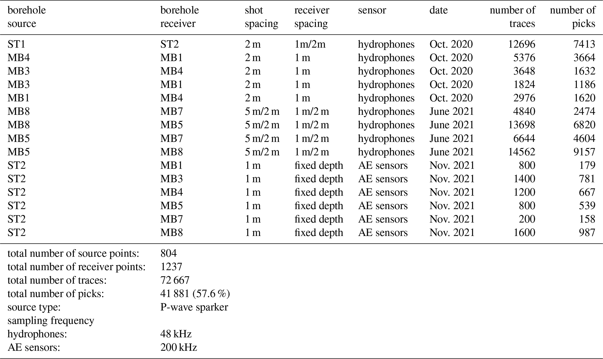
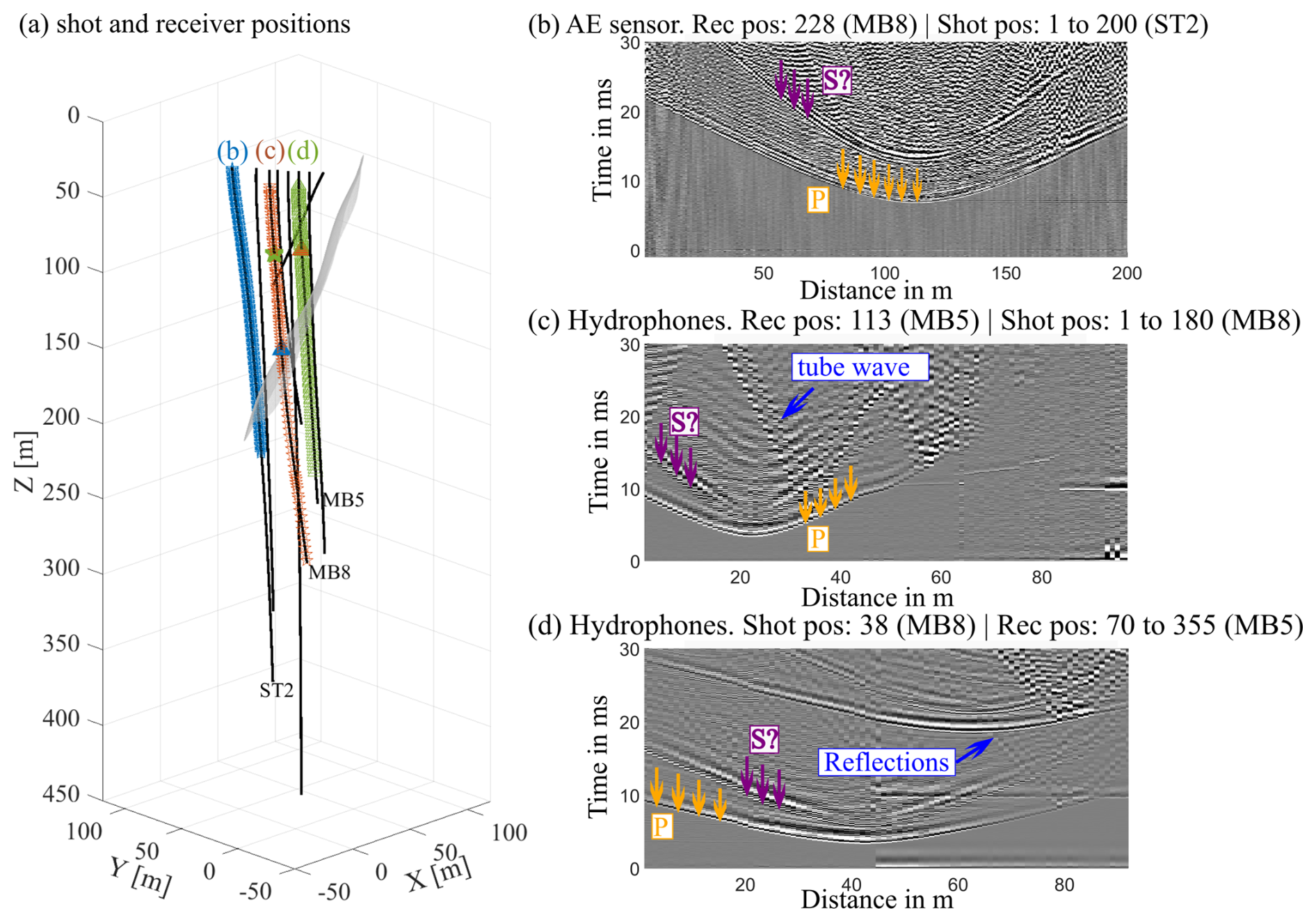
Figure 2 Experimental setup and data examples. (a) shows the shot (stars) and receiver (triangles) positions for the waveforms shown in (b), (c) and (d). The gray surface indicates the MFZ as derived by Escallon et al. (2024). (b) displays the waveforms recorded by one AE sensor in borehole MB8 (blue triangle) from shots in borehole ST2 (blue stars). (c) shows a corresponding receiver gather recorded on a hydrophone in MB5 (brown triangle) and shots in borehole MB8 (brown stars). (d) shows a shot gather from a source in MB8 (green star) with hydrophones in MB5 (green triangles). First arrivals for P-wave are indicated with yellow arrows, and examples for reflections and tube wave are indicated with blue arrows. The predicted S-wave arrivals are indicated with purple arrows.

We employed a seismic P-wave sparker source with a dominant frequency band of about 1 to 10 kHz (https://geotomographie.de, last access: 11 February 2026). The first three data sets were recorded on two hydrophone chains with 1 and 2 m spacing, respectively (Table 1). The surveys were designed such that the receiver/shot spacing is denser around the MFZ and sparser at distances further away. These initial surveys were conducted before the instrumentation and cementation of the boreholes. The last survey was carried out in November 2021, after instrumentation but prior to the stimulation experiments. Permanently installed acoustic emission (AE) sensors were used as receivers, which had to be synchronized with the sparker setup. For each source point and all surveys, the sparker source was fired three times; the traces were then stacked to enhance the signal-to-noise (SNR) ratio. Overall, we were able to compile a relatively large data set including 41 881 manual P-picks (Table 1) with an average picking uncertainty of about 0.15 ms. Based on visual inspections during the manual picking process. Source-receiver offsets varied between 10 and 186.5 m. For the manual picking we employed a Matlab-based in-house software. Figure 2 shows three examples of shot and receiver gathers: Fig. 2a) gives the setting with the source and receiver configurations as well as the MFZ; Fig. 2b displays a receiver gather recorded on the AE sensors (sensor in MB8, sources in ST2); Fig. 2c shows a receiver gather recorded on a hydrophone (sensor in MB5 and receiver in MB8) and Fig. 2d shows a source gather recorded on hydrophones (source position in MB8 and receivers in MB5). The first arrivals of the P-waves, indicated by the yellow arrows, are clearly visible. The P-wave sparker, as the name suggests, is designed to generate primarily seismic P waves. S waves that are visible in the data are therefore most likely converted P-to-S phases, with the conversion probably taking place at the source borehole wall. The S waves are marked in Fig. 2b, c, and d (purple arrows). They are generally difficult to pick because they often overlap with scattered parts of the P waves or with reflected waves. Therefore, we restrict ourselves to the first arriving P waves. Figure 3a shows example traces from a hydrophone and an AE sensor with a similar source-receiver offset. Both traces show a high signal-to-noise ratio. To further appraise the properties of the seismic waveforms, we computed sum spectra for the hydrophone and AE sensor data. For that purpose, all traces where we could pick the first break of the P wave were considered. A time window of 6 ms around the first break was used to calculate the amplitude spectra (gray boxes in Fig. 3a). The amplitude spectra of the individual traces were then summed to obtain the sum spectra.

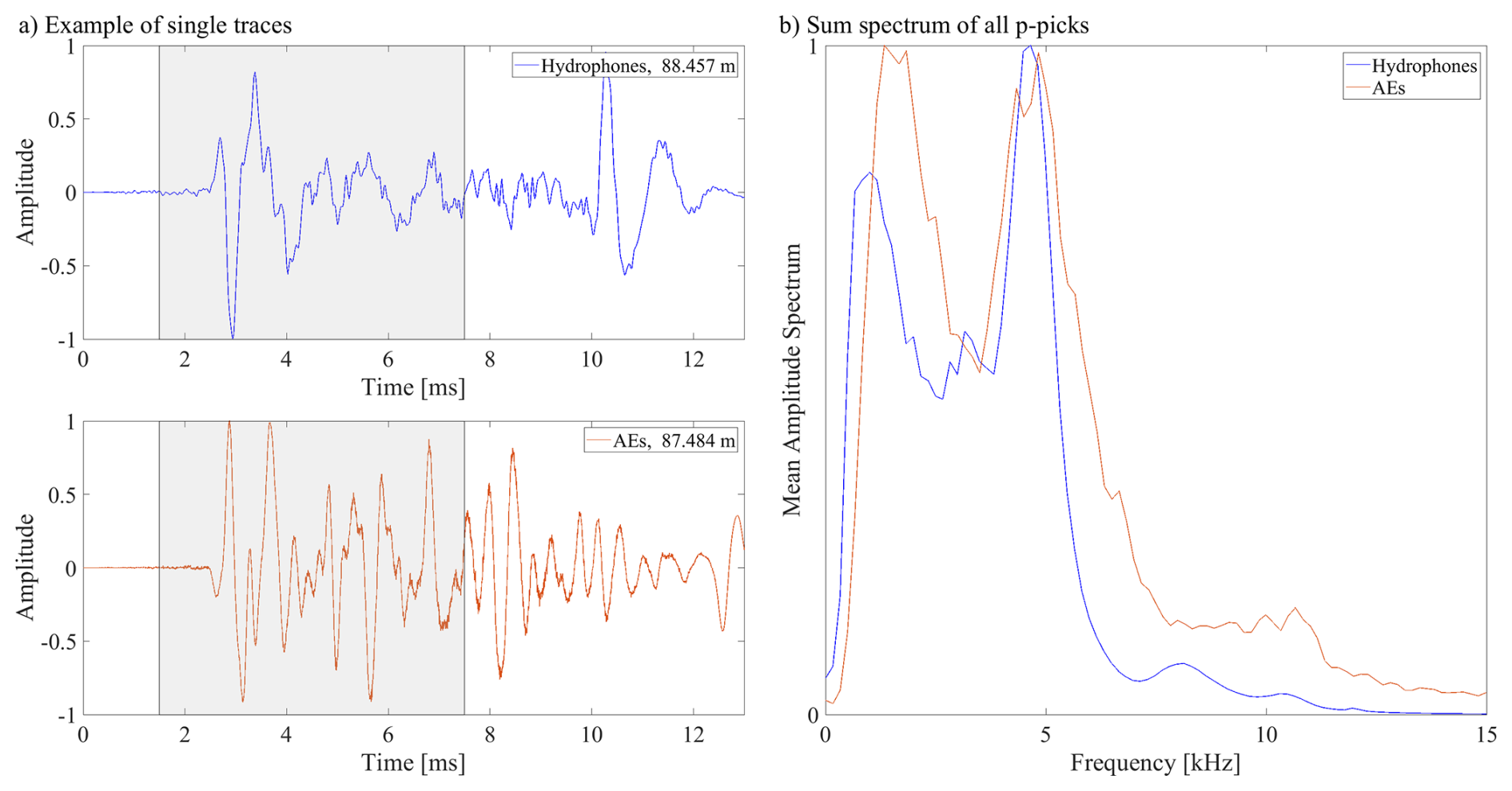
Figure 3 (a) Example traces of a hydrophone (top) and an AE sensor (bottom) that were recorded at similar source-receiver offsets. The gray boxes indicates the time window that was used to calculate the sum spectra shown in (b). For visualization purposes, we normalized the data to the maximum amplitude. (b) shows the sum spectra of all traces with a P pick (see main text for further explanations on the computation of the sum spectra).

The frequency content of both sensor types is comparable, with the energy of the first-arriving waves varying between 1 and 7.5 kHz. It should be noted that the sharp decrease below 1 kHz is caused by the analog filters of the acquisition systems. Furthermore, it is noteworthy that there is a significant decrease of spectral amplitudes around 3 kHz for both sensor types. One may argue that this feature in the sum spectra is caused by the sensor properties or by the acquisition system. However, this feature is visible independently of the recording system (sensor and acquisition system). Since the type of the source does not change, we conclude that the shape of the sum spectra might be caused by the properties of the host rock, for example by the intrinsic attenuation, or the properties of the seismic source. More analyzes, which are beyond the scope of this paper, will be required to further analyze the frequency spectra.

4 Travel time tomography

4.1 Method

Seismic travel time tomography is a well-established method for delineating subsurface structures at various scales (e.g., Nolet, 1987). It requires (i) an initial model, (ii) a forward solver to predict the travel times for a given model, (iii) an inverse solver to estimate the seismic velocities (respectively the seismic slownesses, the inverse of velocity) from the observed data, and (iv) a regularization scheme to account for the underdetermined components of the inverse problem (e.g., Menke, 1984). For our computations, we employed in-house tomography software that includes the algorithm by Podvin and Lecomte (1991) as a forward solver, which solves the Eikonal equation on a regular grid with a finite-difference approach. The seismic rays are then computed with a backtracing algorithm following Li et al. (2018). The accuracy of the forward solver is governed primarily by the discretization of the finite-difference grid (e.g., Podvin and Lecomte, 1991). To solve the inverse problem, the volume of interest needs to be discretized into 3D blocks of adequate sizes. In contrast to the forward solver grid, which is governed by the accuracy of the Eikonal solver, the inverse grid is governed by the spatial resolution power offered by the source-receiver distribution. Therefore, the forward and inversion grids do not necessarily have to be identical. The ray segment lengths for each inversion cell and source-receiver pair are determined and fed into the n×m Jacobian matrix J, where n is the number of data points and m is the number of inversion cells. Since such tomographic problems always include an underdetermined component, regularization of the inverse problem is required. For that purpose, we have added damping and smoothing constraints (see Maurer et al., 1998 and Lanz et al., 1998 for further details). The inverse problem can then be written as

$$\begin{array}{}\text{(1)}& \left(\begin{array}{c}\mathbf{J}\\ \mathbf{D}\end{array}\right)\mathbf{\text{s}}=\left(\begin{array}{c}\mathbf{t}\\ \mathbf{h}\end{array}\right),\end{array}$$

where J is the Jacobian matrix, t the observed travel times, D and h are the regularization constraints, and s is the unknown slowness. As described, for example, in Maurer et al. (1998), matrix D is composed of an upper part, including an m×m diagonal matrix, which is required for the damping constraints, and a lower part, containing an m×m matrix, representing the smoothing operator. Likewise, the vector of h contains an upper part with the initial slowness (first iteration) or the slowness of the previous iteration, and a lower part including zeros. The resulting system of equations in (1) is typically very sparse and can thus be solved conveniently with the LSQR algorithm proposed by Paige and Saunders (1982). With the updated velocity model, the predicted travel times and the ray geometry need to be recomputed to update J. This procedure is then repeated until convergence is achieved. Since infinitely thin rays, computed with the Eikonal equation, are not a good physical representation of finite-frequency seismic waves, and they may not cover all inversion cells, the concept of fat rays was introduced by Woodward (1992). The underlying idea of this concept is to extend the thin rays to a width that corresponds to the dominant wavelengths of the data observed. When the travel time fields from the solution of the finite-difference Eikonal solver are available, the region of the fat rays can be calculated swiftly with the formula of Červený and Soares (1992) that describes the first Fresnel volume, which is equivalent to the fat ray

$$\begin{array}{}\text{(2)}& \mathrm{|}{t}_{\mathrm{sx}}+t_{\mathrm{rx}}-t_{\mathrm{sr}}\mathrm{|}\le T.\end{array}$$

t_sx and t_rx are source or receiver travel times to an arbitrary point x within the forward modeling domain, t_sr is the predicted travel time with the actual model s and T is the dominant period of the seismic waves. When the inequality in Eq. (2) is satisfied, the point x lies within the fat ray volume. To compute the fat ray volumes, it is necessary to not only solve the forward problem for each source position, but also for each receiver position, which can increase the computational costs significantly. For computing the fat ray Jacobian matrix, it is necessary to compute a function f_x for every source-receiver pair, defined as

$$\begin{array}{}\text{(3)}& f_x=\left\{\begin{array}{c}T-t_{\mathrm{sx}}-t_{\mathrm{rx}}+t_{\mathrm{sr}}\text{, if }\mathrm{|}{t}_{\mathrm{sx}}+t_{\mathrm{rx}}-t_{\mathrm{sr}}\mathrm{|}\le T\\ \text{0, otherwise}\end{array}\right.\end{array}$$

at every grid point of the forward model. Then, the f_x values, contained in a particular inversion grid cell, are summed up and inserted into the corresponding element of J. Finally, each row of J needs to be scaled, such that Js=t_sr is enforced.

A beneficial feature of the fat ray approach is that the tomographic results are less dependent on the parameterization of the inversion model. When a relatively fine inversion block discretization is chosen, numerous blocks may not be hit by thin rays. In contrast, fat rays always cover the same volumes, irrespective of the size of the inversion blocks.

4.2 Setup of the inversion

For the travel time tomography we used the data presented in Sect. 3. A homogeneous velocity model of 5300 m s⁻¹ was used as starting model, estimated from the travel time curves of our data. Since the geological observations along the main tunnel and on the borehole cores did not indicate a pronounced layering, we considered that a homogeneous initial model was adequate. The coordinate system was rotated into the main axis system (or principal axis system) of the borehole trajectories to reduce the number of numerical cells. This resulted in a model with dimensions of 72 × 62 × 406 m³. We compared different block sizes for the thin ray-based approach, referred to as “thin ray”. The inversion block size was either 2 m or 1 m, but the forward solver block size was always kept at 1 m. As described in Sect. 4.1, we applied damping and smoothing constraints for the regularization of the inverse problem. The individual contributions of damping and smoothing were determined by a trade-off curve analysis. The results are shown in Fig. 4. The intersection of the trade-off curve with estimated picking accuracy (dashed black line in Fig. 4), indicates the preferred damping value. A damping/smoothing ratio of 0.5 was found to be adequate for our setup. We repeated the trade-off analysis for other damping/smoothing ratios, and they led to similar results as shown in Fig. 4. Generally, the choice of the regularization parameters proved to be not too critical. Inversions within a range of damping factors around the chosen value led to very similar results, thereby proving the robustness of our inversion setup.

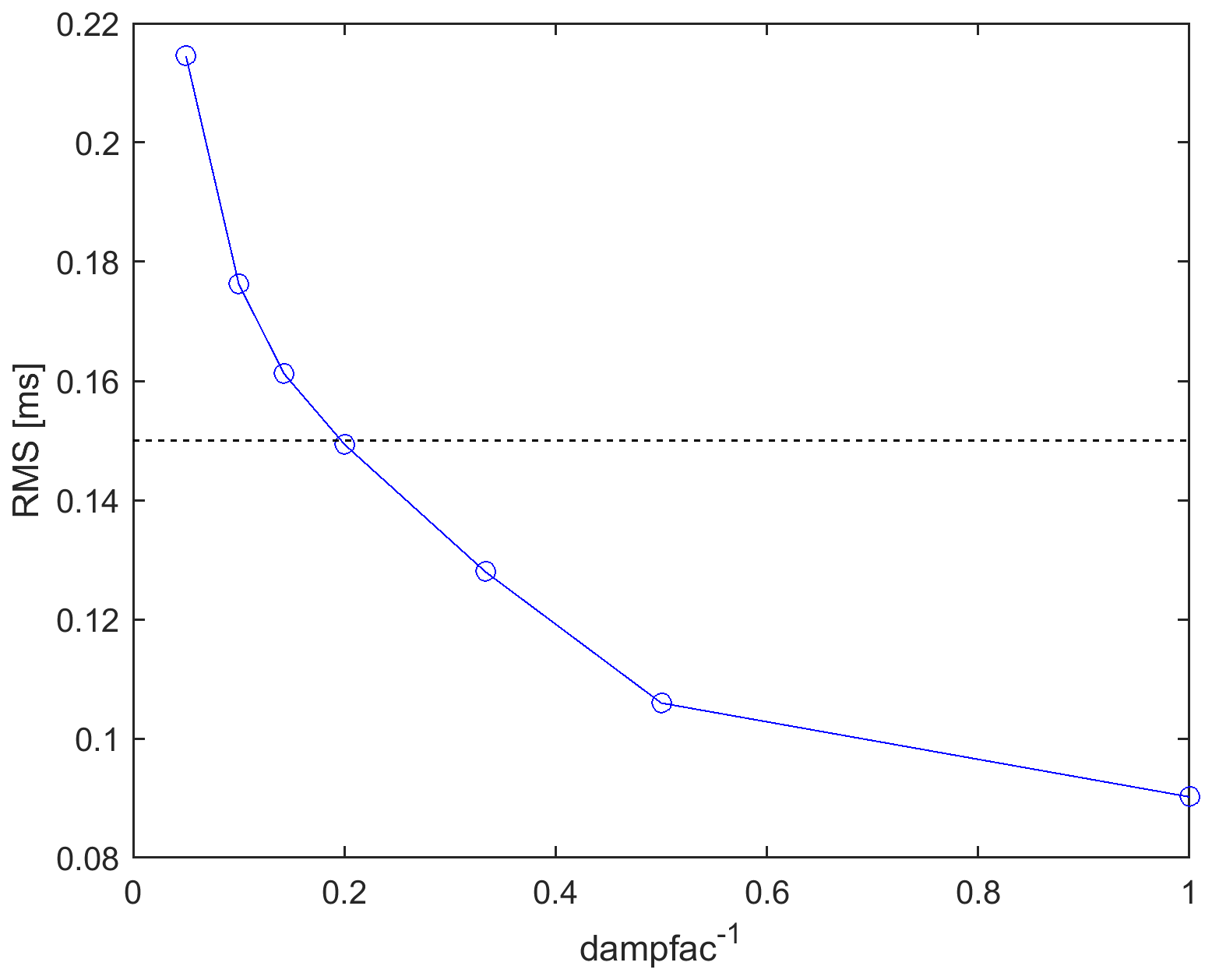
Figure 4 Trade-off curve for determining the regularisation parameters. The horizontal axis denotes the inverse of the damping factors tested during the trade-off analysis. The horizontal dashed line indicates the estimated picking accuracy.

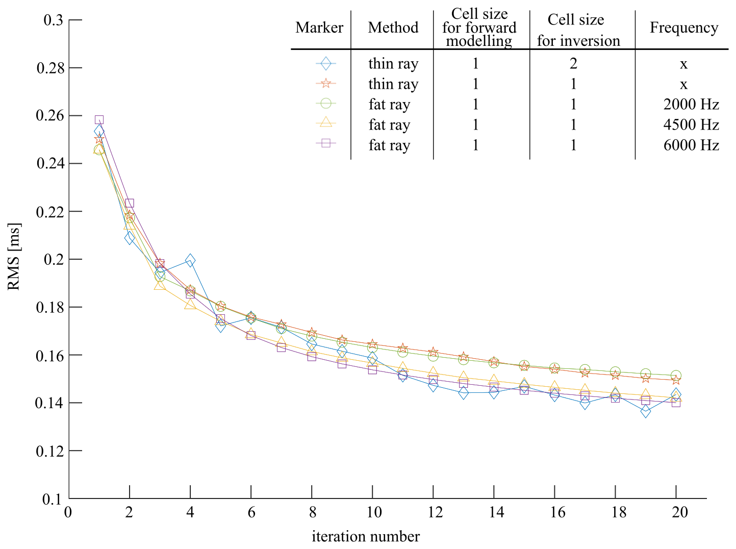
Figure 5 Development of the RMS discrepancy between observed and predicted travel times for different configurations: the thin ray based tomography with two different cell sizes of the inverse solver (1 and 2 m) and the fat ray-tomography with different frequencies, 2, 4.5 and 6 kHz. Fat ray inversions employed the same grid for the forward solution and inversion, 1 × 1 × 1 m³. The same applies to the thin ray 1-1 inversion. For the thin ray 1-2 inversion, 8 forward cells were merged to larger cubic inversion cells.

The convergence behavior of the different inversion runs is shown in Fig. 5 in the form of Root-Mean-Square discrepancies between the observed and predicted travel times (RMS curves). For the fat ray tomography, we always used the smaller inversion cell size of 1 m and compared different frequencies: 2, 4.5 and 6 kHz that are within the frequency spectra of the P wave (see Fig. 3). With appropriate regularization for the different inversions, all inversion runs converged reasonably well, that is, the RMS curves were flattening out, and all show a similar convergence behavior. However, for the thin ray inversion with a 1 m cell size and for the fat ray inversion with 4.5 and 6 kHz, more regularization was required to account for the larger underdetermined component of the inversion problem (the magnitudes of D and h in Eq. 1 were increased by 50 %). Generally, the RMS reduced from 0.25 ms to approximately 0.15 ms within 20 iterations, which is consistent with our picking accuracy. Since no significant differences were observed in the convergence behavior of the different settings and the resulting tomography models were similar, we selected 2 kHz for our fat ray tomography to obtain the best spatial coverage with the lowest reasonable frequency.

4.3 Comparison of Thin ray and Fat ray tomography

To show the benefit of the fat ray approach, we compare the 2 kHz fat ray results with the thin ray results. For the comparison, we consider not only the velocity structures but also the column sums of the Jacobian matrix, subsequently referred to as “coverage”, as described, for example, in Jordi et al. (2016). The summation of the jth column of the Jacobian matrix gives an estimate of the overall sensitivity related to the jth inversion cell. The “coverage” measure is similar to the ray-coverage that is often used in thin ray tomography. To emphasize that we calculate the fat ray coverage from the column sums of the Jacobian matrix, we consistently use the term “coverage” throughout the paper. In Fig. 6, we compare the velocity tomograms for the thin ray (Fig. 6a) and the 2 kHz fat ray (Fig. 6b) at a horizontal slice at z=150 m. Higher velocities are displayed in blue, lower velocities in red, and the mean velocity (≈5340 m s⁻¹) is represented in gray. Areas with insufficient or no coverage are shown in white. The green line indicates the MFZ at this depth. Both tomograms show similar features, but the structures in the fat ray tomogram (Fig. 6b) are much clearer. Note, for example, the low-velocity anomalies around MB8, and between ST1 and ST2. Furthermore, the area covered with fat rays is considerably larger, and it does not include any gaps. Considering the fact that fat rays are a better physical representation of the actual finite-frequency wavepaths, one can conclude that the tomogram in Fig. 6b) is not only clearer but also likely more reliable. The corresponding coverage plots are shown in Fig. 6c and d.

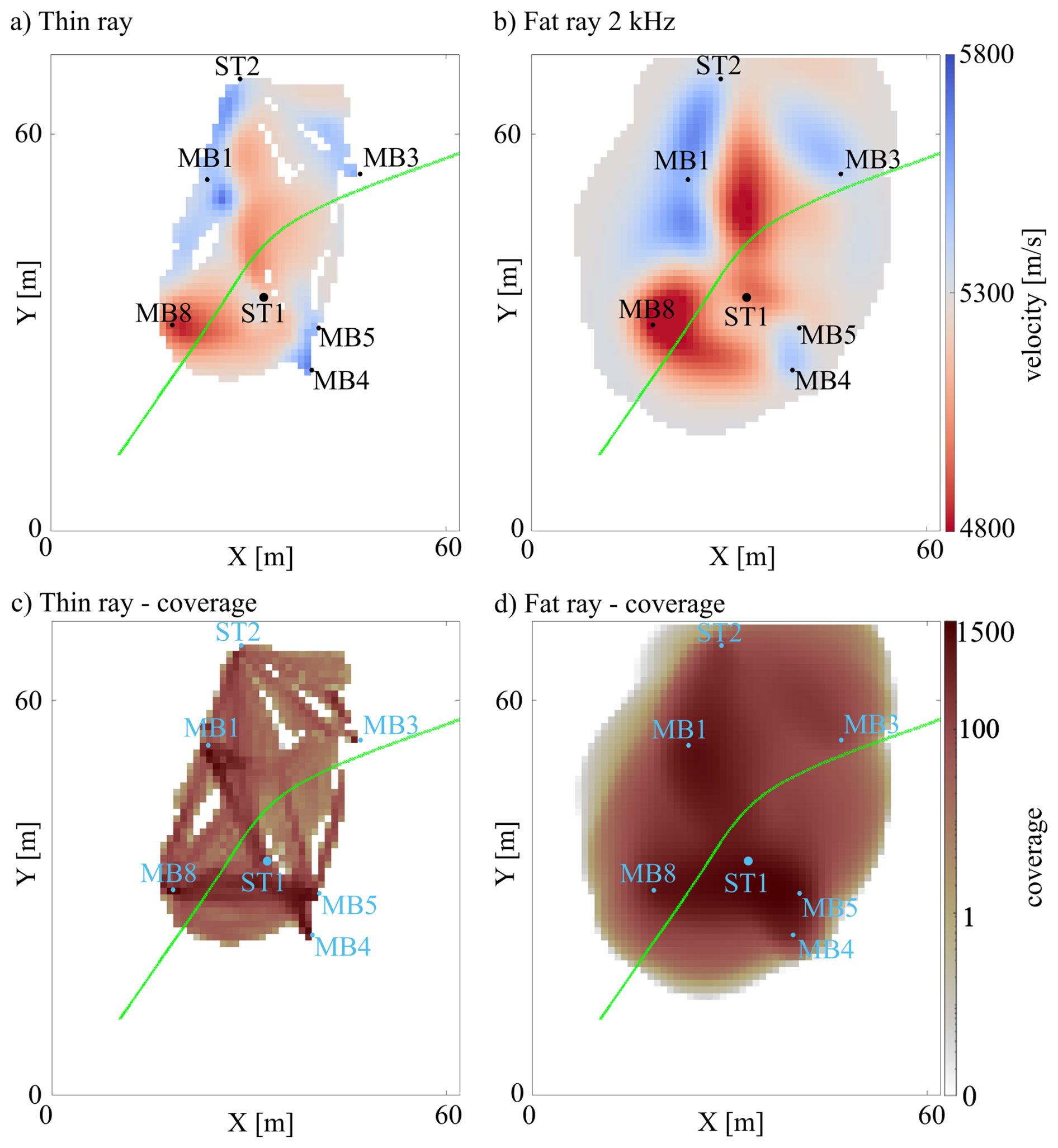
Figure 6 Comparison of thin and fat ray tomography using an x–y slice at z=150 m: (a) tomogram of the thin ray approach, (b) tomogram of the 2 kHz fat ray approach. The intersections of the boreholes with the slice are also marked. (c) and (d) show the coverage, defined using the column sums of the Jacobian matrix. We applied the colors such that white shows no coverage, and gray to yellow extremely low; higher coverage values are represented using a red colormap ranging from light to dark red.

5 Application to field data set

5.1 Qualitative description of the 3D velocity model

In this paper, we consider only the velocity model obtained with fat ray tomography using a center frequency of 2 kHz. The velocity models obtained with 4.5 and 6 kHz do not show significantly better results; for example, the RMS curves are quite similar (Fig. 5). Therefore, we chose the lowest reasonable frequency to obtain the best coverage. The P-wave velocities in this tomographic model vary between 4685 and 6212 m s⁻¹, and the mean velocity is approximately 5340 m s⁻¹. Fig. 7a shows the tomographic velocities, and the corresponding coverage is shown in Fig. 7b) at different depths (z-axis). The intersections with the boreholes are shown as black dots in (a), and blue dots in (b). The intersection of the slice with the MFZ is marked with a green line.

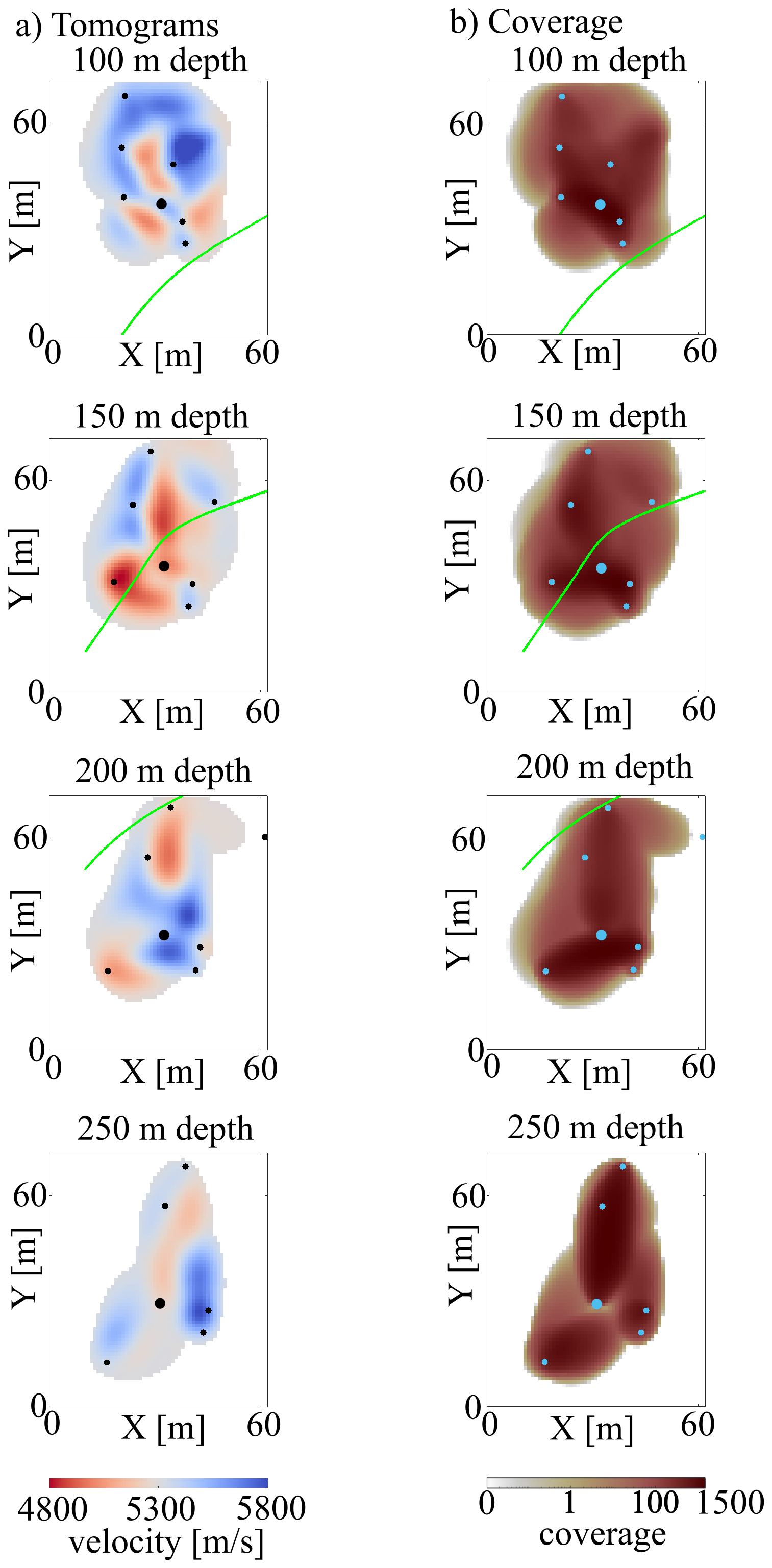
Figure 7 (a) Velocity tomograms at different depths and (b) the corresponding spatial coverage. Unresolved areas are left white. The dots indicate the intersections of the boreholes with the slice; the larger dot indicates borehole ST1. The green line indicates the intersection with the MFZ. As in the previous plot, white shows no coverage, and gray to yellow extremely low, higher coverage values are represented using a red colormap ranging from light to dark red.

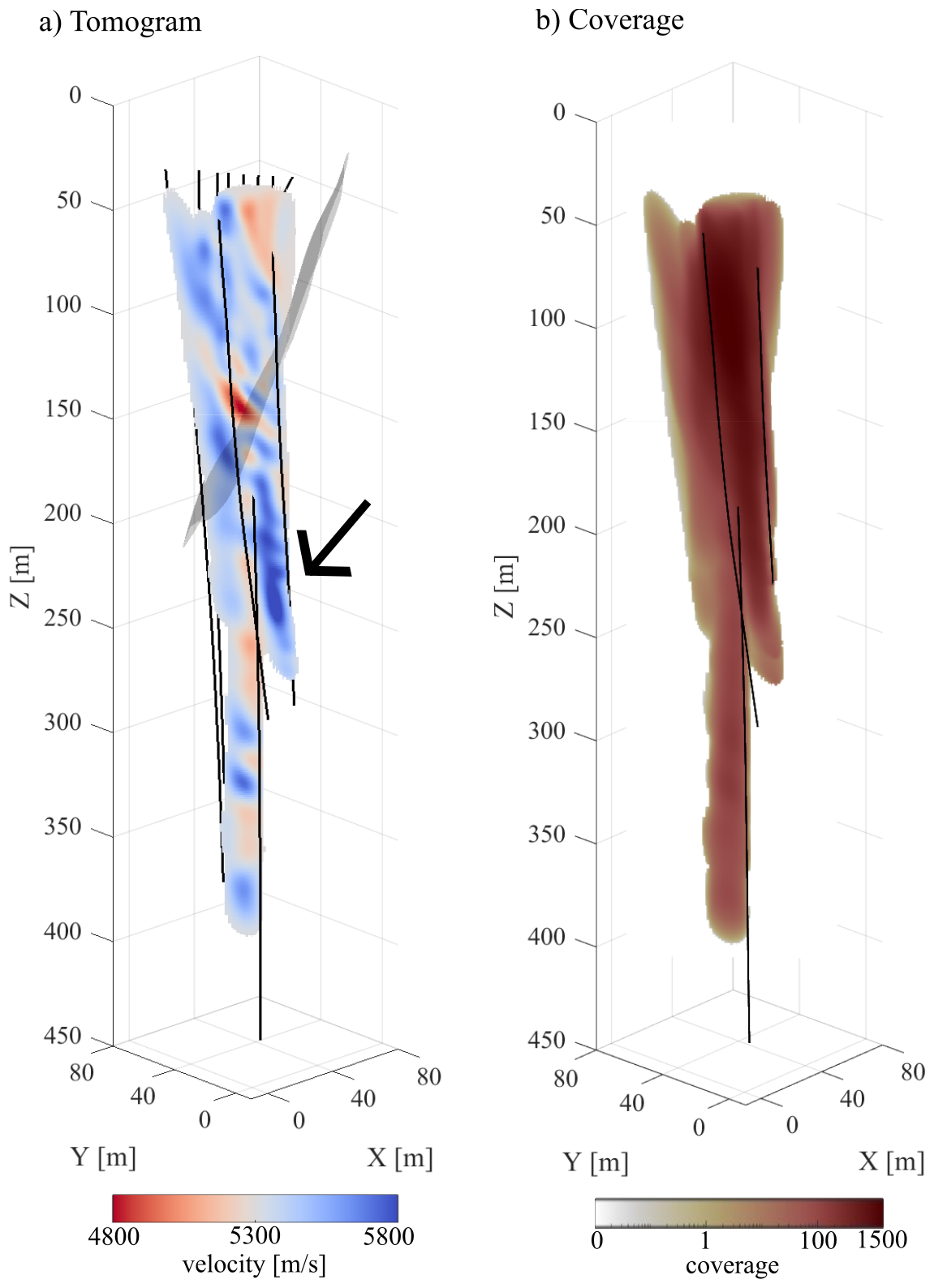
Figure 8 (a) Vertical slice perpendicular to the MFZ, which is shown as gray surface. The zone with particularly high velocity is marked by a black arrow. (b) shows the same slice as (a) but is the coverage of the model. As in to the previous plots, we use the following colormap for the coverage: white shows no coverage, and gray to yellow extremely low coverage. Higher coverage values are represented using a red colormap ranging from light to dark red.

At z=100 m, we generally observe the highest velocities of all slices. This area is distinguished by largely intact granites (Bröker et al., 2024a). At z=150 m, we observe a low-velocity feature in the region, where the MFZ intersects the slice. At z=200 m and z=250 m, we observe several low- and high-velocity zones. The coverage plots in Fig. 7b indicate that all these features are potentially well constrained by the data (see checkerboard tests in Appendix A).

A vertical slice through the model is provided in Fig. 8. Since the MFZ (see Fig. 1c) is a feature of major interest, we provide a vertical section perpendicular to the strike of this fault zone through the central part of the 3D model. The vertical section confirms that there are predominantly low velocities between z=100 m and z=150 m, while generally higher velocities are observed at greater depths (see, for example, the region marked by black arrow in Fig. 8a). Below z=250 m, the coverage and thus the reliability of the velocity model is limited.

The horizontal and vertical slices in Figs. 7 and 8 provide some insights into the structure of the 3D velocity model. However, such single slices can be difficult to interpret. Therefore, we created a series of videos, making it possible to scan in various directions through the model cube. These videos are provided in the digital appendix, and we highly recommend that the reader make use of them to better understand the structures contained in the 3D model.

The horizontal and vertical slices in Figs. 7 and 8 indicate that there are hints of the MFZ (e.g., the low-velocities near the MFZ intersection at z=150 m in Fig. 7), but there are no consistent manifestations of it in the 3D velocity. This can either be indicative of a high degree of complexity of the MFZ, but it could also be due to insufficient spatial resolution of the tomograms. To address the latter, we performed a series of checkerboard tests that are documented in Appendix A. In brief, the tests demonstrated that the spatial resolution lies between 5 and 10 m, with decreased resolution towards the borders of the regions with insignificant coverage.

5.2 Travel time residuals

To quantify how well the 3D tomographic velocity model explains the observed travel times, we superimpose the observed and predicted travel times in Fig. 9a as a function of source-receiver offset. For a better visualization, the travel times t_eff are shown in reduced form, that is, $t_{\mathrm{red}}=t_{\mathrm{eff}}-\mathrm{\Delta }/v_{\mathrm{red}}$, where Δ is the source-receiver offset and v_red is the reduction velocity, which we have chosen to be 5340 m s⁻¹. Consequently, travel times with a ray velocity of v_red plot along a horizontal line at t_red=0. Additionally, we show the differences between the observed and predicted data (residuals) as a function of source-receiver offset (Fig. 9b) and in form of a histogram (Fig. 9c). From the residual plots in Fig. 9b, two main conclusions can be drawn. First, there seems to be no significant offset-dependent variations of the residuals (such variations could be indicative of systematic errors in the tomograms). Second, about 70 % of the residuals are below the average picking accuracy of 0.15 ms (marked with solid black lines in Fig. 9b and c). Therefore, the standard deviation of the residual distribution is close to the average picking accuracy, indicating that the observed data are neither over- nor under-fitted by the 3D tomographic velocity model.

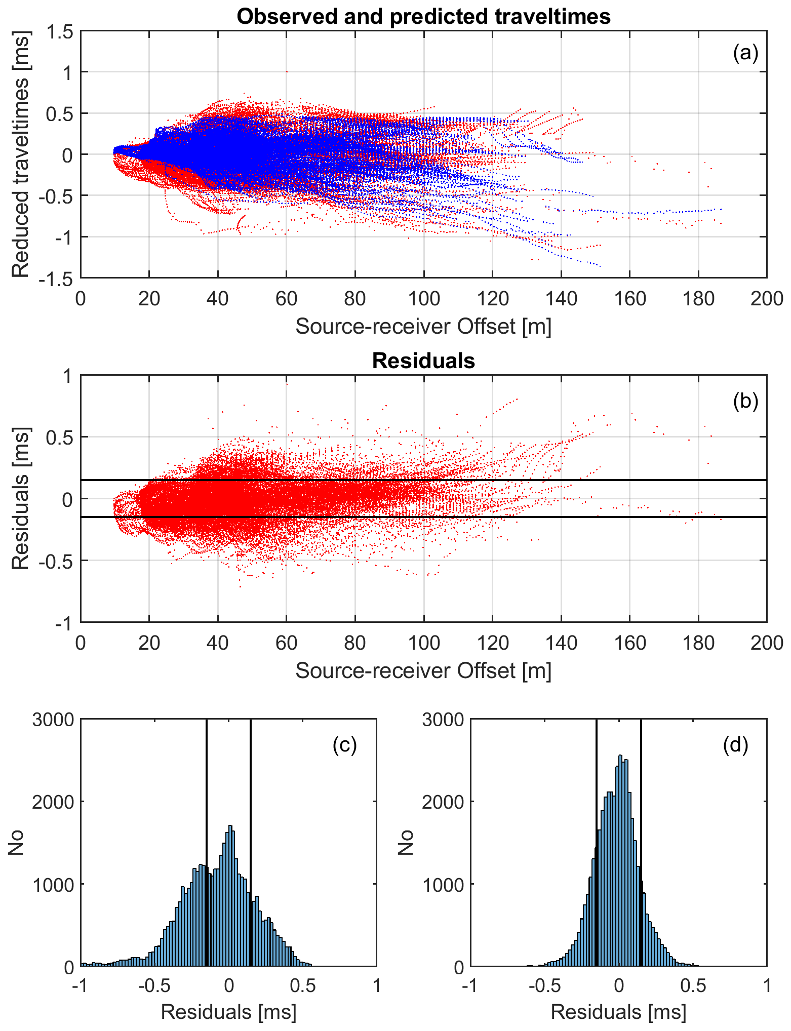
Figure 9 (a) Observed (red) and predicted (blue) travel times as a function of source-receiver offset. Reduced traveltimes are defined as $t_{\mathrm{red}}=t-\mathrm{sro}/\mathrm{5340}$, where t_red and t denote the reduced and actual traveltimes, and sro is the source-receiver offset. (b) Corresponding residuals plotted as a function of source-receiver offset. (c) Residuals shown in form of a histogram. The manually determined picking accuracy is indicated with solid black lines in (b) and (c).

5.3 Validation of the velocity model with independent data sets

Laboratory measurements at fluid-saturated undisturbed core samples indicate velocity values up to v_p=5434 m s⁻¹. From these results, the P-wave velocities at in-situ conditions with P_eff=15 MPa are estimated to be 6123 m s⁻¹ (David et al., 2020). This is broadly consistent with the maximum values of the tomograms (6212 m s⁻¹). Another option for validating the velocities obtained by the tomographic inversions is offered by sonic logs, acquired in borehole ST1. A comparison is shown in Fig. 10. To compare both data sets, the sonic logs were downsampled to the sampling rate of the tomographic velocity model. The tomographic velocities are shown in black and those of the sonic logs are shown in orange. Adjacent to the velocity profiles, we also extracted the coverage (defined via the column sums of the Jacobian matrix) along the coordinates of ST1, shown as blue line. They show that the depth range of trustworthy tomographic velocities lies between 50 and 230 m (denoted by horizontal dashed lines in Fig. 10). As a consequence, the tomographic velocities above and below the resolved depth range are close to the initial velocities of 5300 m s⁻¹.

In the resolved depth range, the sonic logs show slightly higher velocities compared with the tomographic results. This is expected because the sonic logs employ higher frequencies. Therefore, the comparison with the sonic logs is rather restricted to relative velocity changes. Both curves show a significant low-velocity anomaly at about 150 m depth. To verify this low-velocity zone as a feature of the MFZ, we compare it with the ATV (Acoustic Televiewer Log) measurements (Fig. 10, right panel) at this depth. We show the ATV travel times, adapted from Bröker et al. (2024a). The ATV measurements reveal a broad fracture zone shown by an increase in ATV travel time up to 180 µs. Furthermore, Bröker et al. (2024a) provide more evidence for the existence of a significant fracture zone. Spinner, electrical conductivity, and temperature logs exhibit very significant anomalies in this depth range. Furthermore, optical televiewer measurements indicate smaller breakouts.

The velocities of the 3D tomography model, extracted along the ST1 borehole, generally indicate good agreement with the borehole logs. So the question arises: will the tomographic velocity model allow delineations and characterizations further away from the boreholes, where no ground truth information is available? For that purpose, we again consider the horizontal and vertical slices through the 3D velocity model (Figs. 7 and 8, along with the movies provided in the digital appendix). If the MFZ appears to be a clearly confined zone, one would expect a correspondingly well-confined low-velocity zone in the velocity model. Instead, we generally observe decreased velocities along the MFZ intersections; however, there is also a substantial amount of heterogeneity. At the horizontal slice z=150 m (Fig. 7), the MFZ crosscuts the slice in its central part, where the spatial resolution is best, but at z=100 m and z=200 m, the intersection is at the border of the resolution limit (Fig. 7b). As demonstrated in Appendix A, the resolving power of our data set is limited towards the edges of the regions with coverage. Therefore, it remains unclear whether the heterogeneities are the result of the complexity of the MFZ or if they are caused by the limited spatial resolution. Most likely, both effects contribute to the observed velocity structures.

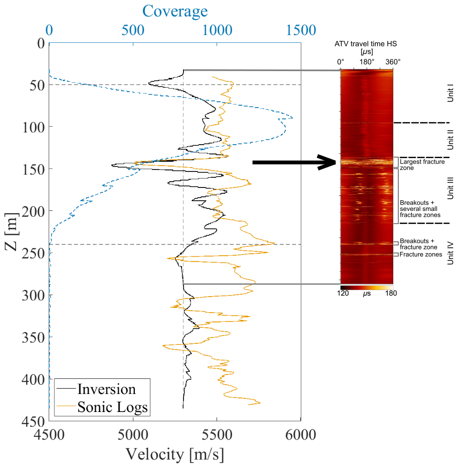
Figure 10 Comparison of the inversion results with additional data acquired along the central borehole ST1 (Fig. 1c). Tomographic velocities, extracted along ST1 (black) are compared with sonic log data (orange). The horizontal gray dashed lines indicate the zone of significant coverage shown with a dashed blue line (between z=50 m and z=250 m). In this range, we compare the results with ATV logs from Bröker et al. (2024a) .

5.4 Appraisal of rock quality

The velocity variations found in the tomographic volume are relatively small, and 99 % of the velocities lie in the range $\mathrm{4900}<v_p<\mathrm{5800}$ m s⁻¹. This is consistent with the findings from borehole logs (Shakas, 2019) that the host rock is moderately disturbed. The velocity variations can be further quantified using the seismic rock quality designation factor (SRQD) introduced by Deere and Miller (1966):

$$\begin{array}{}\text{(4)}& \mathrm{SRQD}={\left({\displaystyle \frac{v_p}{v_p^{\mathrm{lab}}}}\right)}^{\mathrm{2}}\times \mathrm{100}.\end{array}$$

$v_p^{\mathrm{lab}}$ is the velocity of the intact rock measured in the laboratory, which is 6123 m s⁻¹ for the BedrettoLab (David et al., 2020). According to Deere and Deere (1988), the SRQD is a good approximation to the rock quality designation factor (RQD). The SRQD values within our tomographic model lie between 64 and 90, which translates into a rock quality from “fair” to “good/excellent”. This is consistent with geological observations in the geothermal testbed. Based on tunnel observations and borehole logs, Ma et al. (2022) conclude that the general amount of fracturing in the geothermal testbed is low to moderate.

5.5 Limitations of the tomographic velocity model

For an appropriate interpretation of the structures found in the 3D tomographic model, it is necessary to consider its inherent limitations. First, the spatial resolution should be considered. This is influenced by the coverage within the model and the seismic wavelengths. As shown in Figs. 7 and 8, the coverage of the fat rays is generally high and homogeneous. Williamson and Worthington (1993) demonstrated that the spatial resolution scales approximately with the width of the Fresnel zone. Using an average velocity of the tomographic model, a frequency of 2 kHz and an average source-receiver distance of about 50 m, the width of the Fresnel zone is approximately 10 m, which corresponds quite well with the minimum feature size in the fat ray tomograms. Furthermore, this is remarkably consistent with the results of the checkerboard tests documented in Appendix A.

Additional factors that may limit the reliability of the tomograms include the presence of seismic anisotropy and the accuracy of the borehole traces. As indicated earlier, minor anisotropy effects may exist, but we have chosen to employ an isotropic model. Ignoring significant anisotropy effects during an isotropic inversion would produce layered structures with alternating high and low velocities, thereby mimicking anisotropy. We did not observe a pronounced layering in our tomograms.

Another potential source of systematic errors includes inaccuracies of the borehole trajectories, which tend to increase towards the bottom of the boreholes. Maurer and Green (1997) showed that such deviations from the true trajectories would result in substantial anomalies near the borehole bottoms, where the formal resolution is lowest and anomalies can be easily developed by systematic errors. Such effects are not observed in our tomograms.

Although we can exclude major artifacts from systematic errors introduced by anisotropy and borehole trajectory inaccuracies, it cannot be excluded that they may have introduced minor distortions. Therefore, only gross features in the tomograms should be interpreted.

5.6 Comparison of seismic velocities with induced seismicity

In 2022–2023, hydraulic stimulation experiments were conducted in the geothermal testbed by injecting water into selected packer intervals of borehole ST1 (see also Sect. 2). An overview of these experiments is provided by Obermann et al. (2024), with a seismic analysis using DugSeis (Rosskopf et al., 2024, 2025). We focus here on the seismicity from Phase I, during which eight intervals at depths of $\mathrm{120}<z<\mathrm{300}$ m were stimulated using consistent injection protocols (Bröker et al., 2024a; Doonechaly et al., 2025). We examine the relationship between seismicity and our 3D tomographic velocity model, and assess the effect of velocity heterogeneity on location accuracy.

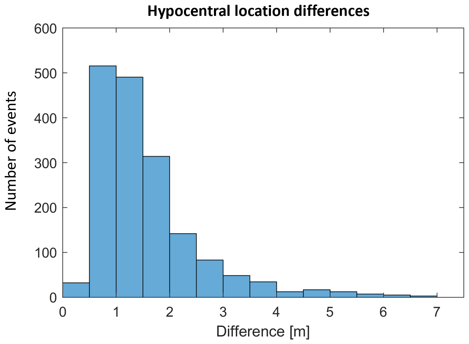
Figure 11 Histogram of the absolute location differences using either a homogeneous or the 3D tomographic model.

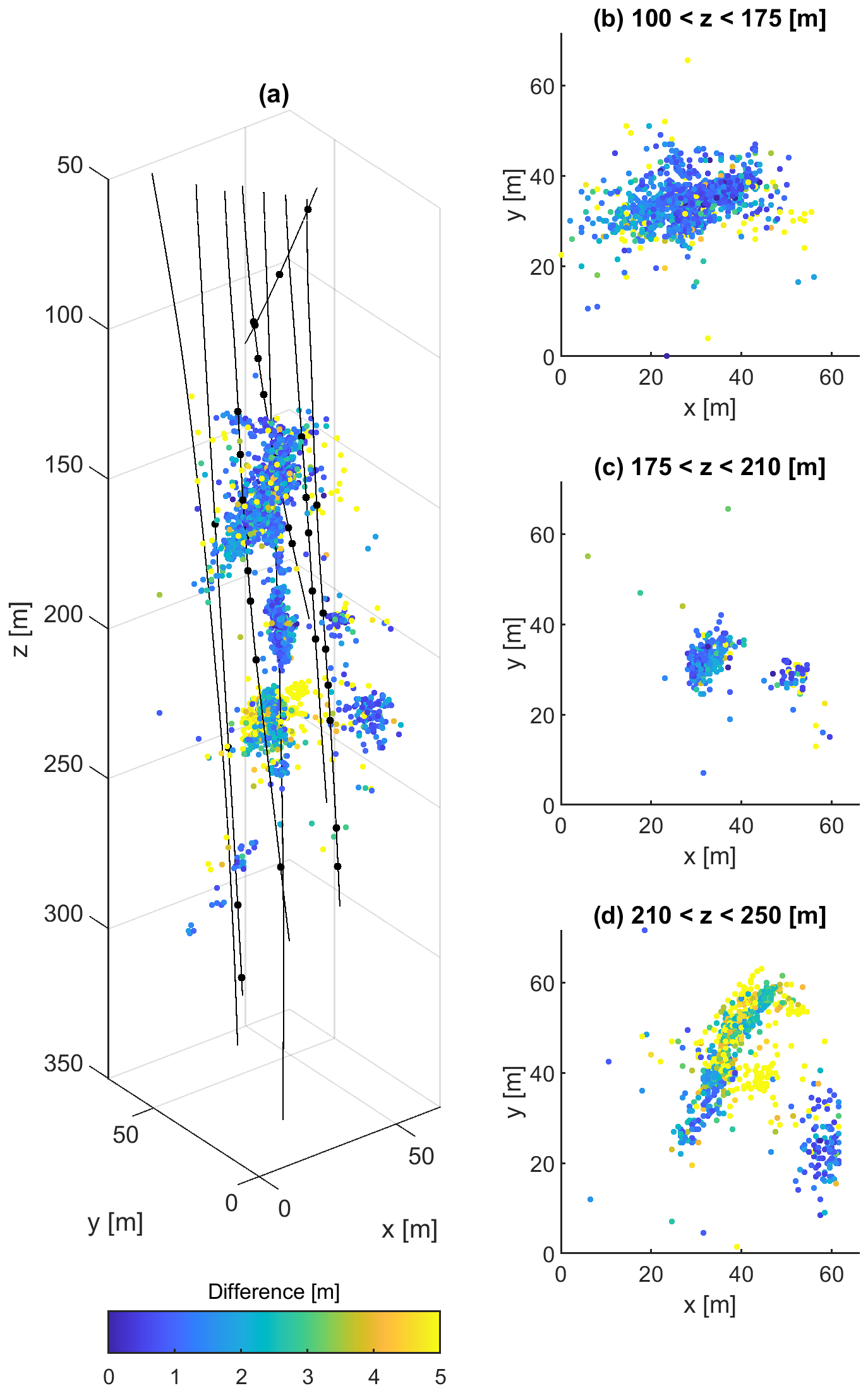
Figure 12 Spatial distribution of location differences shown in Fig. 11. Panels (b) to (d) include top view representations of selected depth intervals.

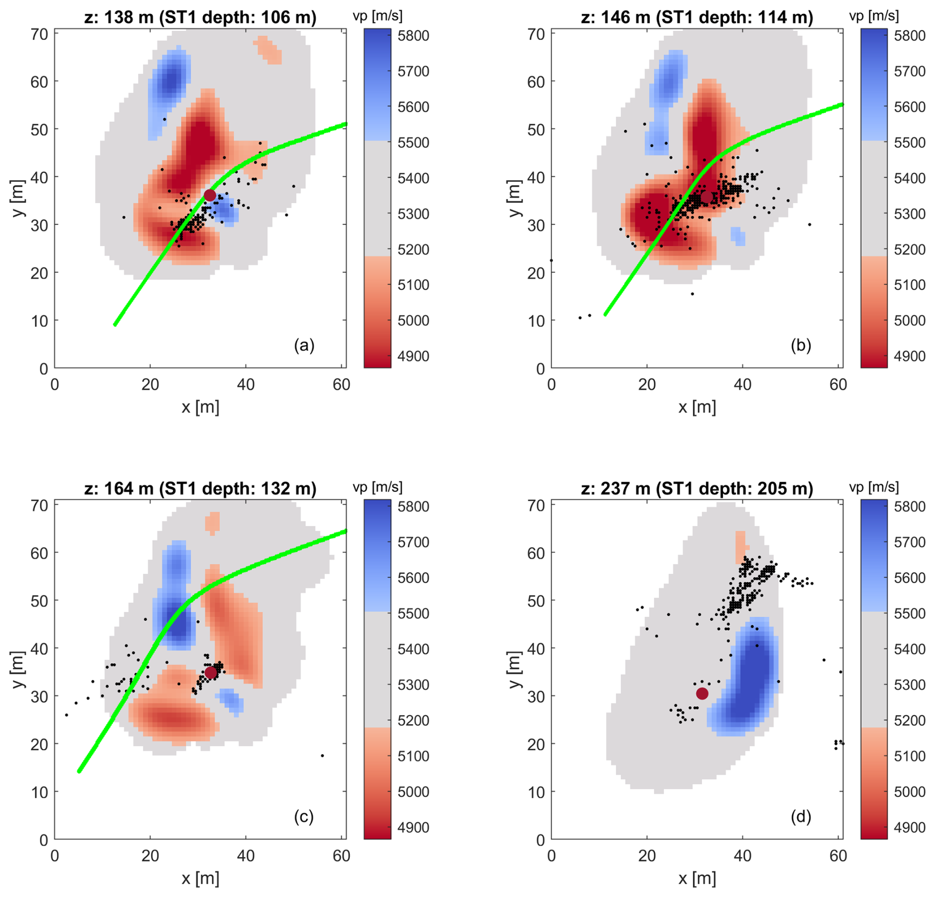
Figure 13 Horizontal slices through the 3D tomographic model. Low and high velocities are shown in red and blue, respectively, and intermediate velocity areas are shown as gray. The seismicity located ±2.5 m distance from the slices is superimposed and indicated by black dots. The intersection of the MFZ is indicated by the green line.

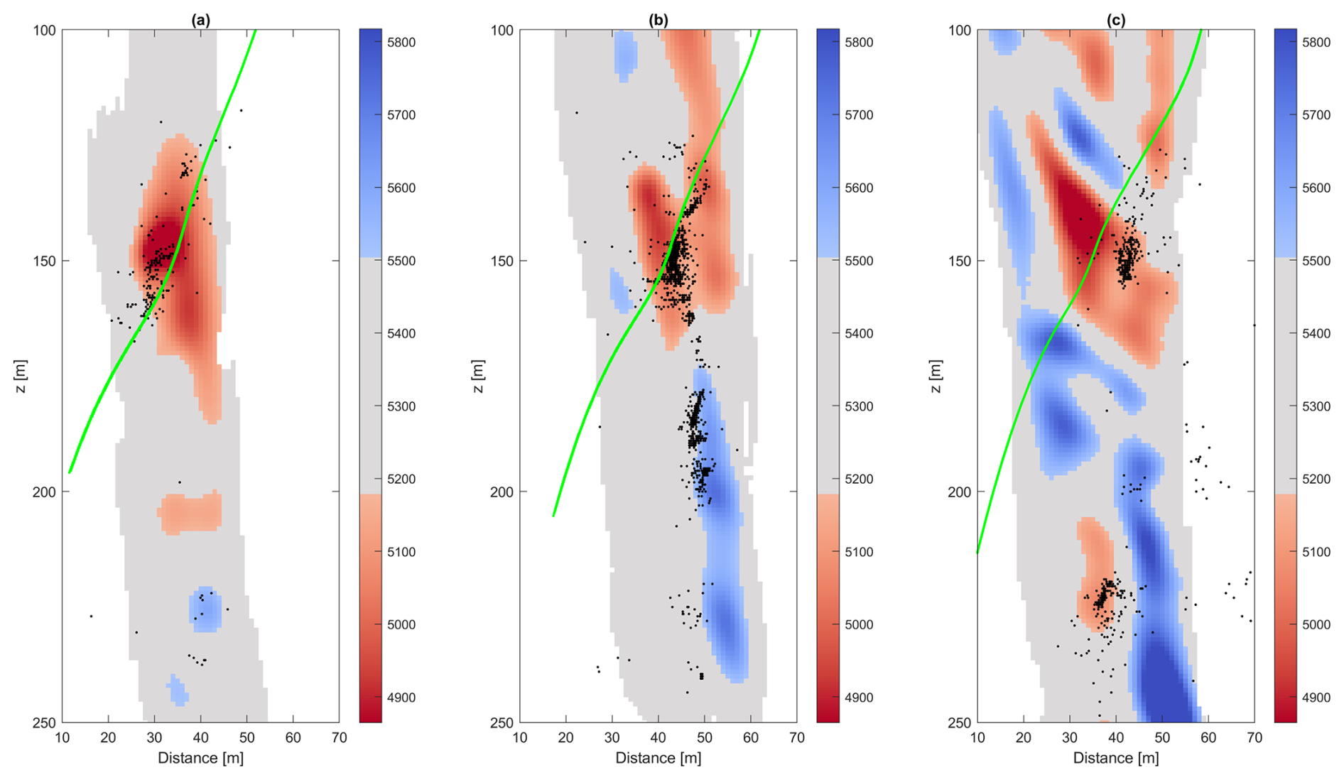
Figure 14 Vertical slices perpendicular to the MFZ through the tomographic model. The slices are located near the trace of the injection borehole ST1 (roughly ±10 m away from each other). Low and high velocities are shown in red and blue, respectively, and intermediate velocity areas are shown as gray. The seismicity located ±2.5 m distance from the slices is superimposed using black dots. The intersection of the MFZ is indicated by the green line.

For the analysis, we selected well-constrained events from the catalog of Obermann et al. (2024), restricted to those within the tomographic model. Events were required to have at least six P-wave picks (no S-wave picks were available) and were relocated using a grid-search algorithm (Moser et al., 1992) with travel times computed via the Eikonal solver (Podvin and Lecomte, 1991) on a 0.5 m grid. Outliers in the pick database were removed using a 0.75 ms threshold, after which the selection criteria were re-applied and events re-relocated. We further excluded events with poor location geometry using the D-criterion (Kijko, 1977), which is proportional to the determinant of the Hessian matrix of the linearized location problem (see Kijko, 1977 for more detailed explanations). Based on visual inspections, we have chosen a threshold of $\mathrm{1}\times {\mathrm{10}}^{-\mathrm{7}}$. This procedure yielded 4283 events out of the original 6413 events for further analysis.

All considered events have moment magnitudes $M_{\mathrm{w}}<-\mathrm{3}$ and can therefore be attributed to the fluid injections within the geothermal testbed, and not to the regional seismicity. Crosshole measurements were performed prior to injection and thus represent pre-stimulation conditions. Repeated active measurements during stimulation indicated P-wave velocity changes well below 1 %.

5.6.1 Influence of the velocity model on hypocentral parameters

Figures 11 and 12 compare event locations obtained with the 3D tomographic model and a homogeneous velocity model with an average velocity of 5340 m s⁻¹, both using the same grid search algorithm. Differences are generally small (mean: 2.2 m, median: 1.4 m), with slightly larger deviations at depth z>210 m. No systematic shift is observed between the event locations using the two velocity models. We therefore conclude, in line with observations from Rosskopf et al. (2025), that velocity variations in the 3D model have only a minor effect on event locations.

5.6.2 Spatial correlation of seismic velocities and the induced seismicity

To study the spatial correlation between seismicity and velocity structures, we employed the following methodology: First, we subdivided the velocity model into low, intermediate, and high-velocity regions. Low and high velocities were defined as values with more than one standard deviation (≈150 m s⁻¹) below or above the mean velocity (≈5340 m s⁻¹). Then, seismic events were superimposed on horizontal and vertical slices of the velocity model, within ± 2.5 m of each slice (Figs. 13 and 14; full slice series in the digital appendix).

Several interesting observations can be made from the superimposed images in Figs. 13 and 14. In horizontal slices at injection depths, the seismicity clusters around the injection borehole ST1, with little correlation to the MFZ (green lines in Fig. 13). Most events occur in slightly reduced or intermediate-velocity zones and only very rarely in high- or very low-velocity regions. At z=237 m, a distinct cluster lies about 20 m from ST1, almost entirely in the intermediate velocity range. Vertical slices show similar patterns (Fig. 14): events are concentrated in slightly reduced or intermediate-velocity zones, often along boundaries towards higher-velocity regions.

A possible interpretation of these patterns is that high velocities correspond to intact host rock that remained unfractured under injection pressures (<18 MPa), whereas very low velocities indicate heavily fractured zones incapable of storing sufficient stress. Seismicity thus preferentially occurs in intermediate-velocity zones, where fractures exist but rock strength still allows stress accumulation and failure.

From a mechanical perspective, seismic velocities reflect stiffness. Microcracking and pore fluids lower velocities and stiffness (e.g., Mavko et al., 2009; Paterson and Wong, 2005), consistent with fault-zone observations (e.g., Faulkner et al., 2010) and laboratory rock-failure experiments (e.g., Stanchits et al., 2011). Velocity contrasts likely create strain gradients and stress concentrations at boundaries between intact and damaged rock – a mechanism invoked for acoustic emissions in granite (Salazar Vásquez et al., 2024) and rock bursts in mines (Barton, 2006).

A complementary mechanism is fluid migration: lower- and intermediate-velocity regions are more permeable due to connected microcracks. Fluids preferentially infiltrate these zones, where small pressure perturbations can induce failure if structures are near critical stress (Townend and Zoback, 2000).

We finally checked whether similar correlations between seismicity and intermediate-velocity zones have been observed at other loations and across scales. As already mentioned, they were observed in centimeter-scale laboratory tests (Salazar Vásquez et al., 2024), and similar observations were made at kilometer-scale geothermal fields, e.g. Hengill, Iceland (Obermann et al., 2022). Therefore, we conclude that the spatial correlation between seismicity and intermediate-velocity zones at the BedrettoLab geothermal testbed is consistent with other observations across scales. The most plausible explanations involve stress gradients at velocity contrasts and enhanced permeability in fractured zones. Further work is needed to quantify these mechanisms and link observations with geomechanical processes more directly.

6 Conclusion

The experimental setup of the geothermal testbed in the BedrettoLab offered unique opportunities for 3D tomographic studies. The literature on such investigations at this scale is very sparse; in fact, we could not find a comparable study in the literature. Our findings could thus serve as motivation for other experiments in similar environments.

We showed that, in comparison with traditional thin ray methods, fat ray tomography not only better represents the physics of band-limited seismic data but also provides improved coverage. Furthermore, fat ray tomography is less dependent on the model parametrization of the inversion grid than thin-ray methods, as the sensitivity kernels (i.e., the fat ray volumes) are unaffected by the discretization of the inversion model.

Two main findings emerge from the analysis of the 3D velocity model obtained in this tomography study. First, we were able to characterize a major fault zone. Its signature in the tomographic image is not a narrow and well confined zone of decreased velocities, as one would expect. Instead, it is distinguished by a relatively large volume of generally decreased velocities with considerable heterogeneities. Checkerboard resolution tests indicated that some of these features may result from the limited spatial resolution of our experimental setup, particularly near the boundaries of the region covered by the fat rays.

Second, we observed a spatial correlation between passive seismic events generated by hydraulic stimulations and the velocity structures in our tomographic model. The induced seismic events occur predominantly between high- and very-low-velocity zones. Based on similar results from a small-scale laboratory study, we attribute this observation to the existence of stress gradients in the areas of intermediate velocities.

Appendix A: Checkerboard Tests

The spatial resolution of the tomographic inversions is a key factor for interpreting the 3D tomograms. There are several options that can be considered for appraising the spatial resolution. For seismic tomography, so-called checkerboard tests have established themselves as a useful tool (e.g., Zelt and Barton, 1998). Although such tests have well-known limitations (e.g., Leveque et al., 1993; Rawlinson and Spakman, 2016), they can provide a first-order estimate of the spatial resolution.

To check the resolution power of our data set, we generated synthetic data with block sizes of $\mathrm{5}\times \mathrm{5}\times \mathrm{5}$, $\mathrm{10}\times \mathrm{10}\times \mathrm{10}$ and $\mathrm{15}\times \mathrm{15}\times \mathrm{15}$ m³. The velocity contrasts were chosen to be ±300 m s⁻¹, which reflects the velocity variations found in our tomographic model. The same source-receiver configurations as employed for the inversion of the observed data sets were considered, and the same processing workflows were applied. Similar regularization constraints, as employed for the inversions of the field data, were applied. The results are shown in Figs. A1 to A3. These figures show selected slices through the 3D models. It is evident that block sizes of 15 and 10 m can be generally well resolved, but structures of the size of 5 m remain unresolved in most areas. It is also observed that the spatial resolution decreases, as expected, towards the boundaries of the regions covered by rays. This is particularly apparent in the horizontal slices in Fig. A3. We also repeated the checkerboard tests with the thin ray approach. Similar results as for the fat rays were achieved (not shown).

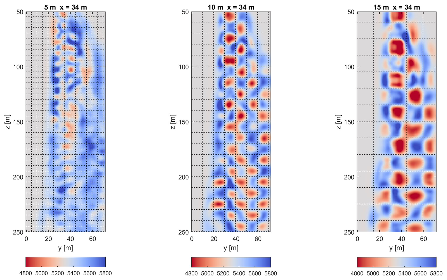
Figure A1 Vertical cross section along a y–z slize at x=34 m. The dashed lines indicate the locations and size of the checkerboard blocks. Block sizes are 5 (left), 10 (middle) and 15 (right) meters.

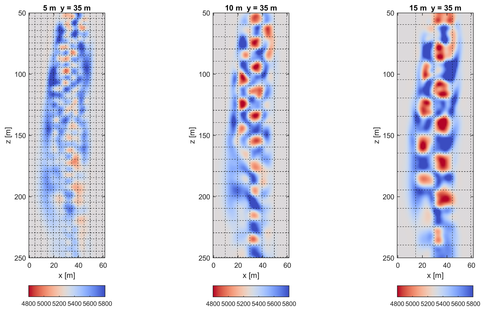
Figure A2 Vertical cross section along an x–z slize at y=35 m. The dashed lines indicate the locations and size of the checkerboard blocks. Block sizes are 5 (left), 10 (middle) and 15 (right) meters.

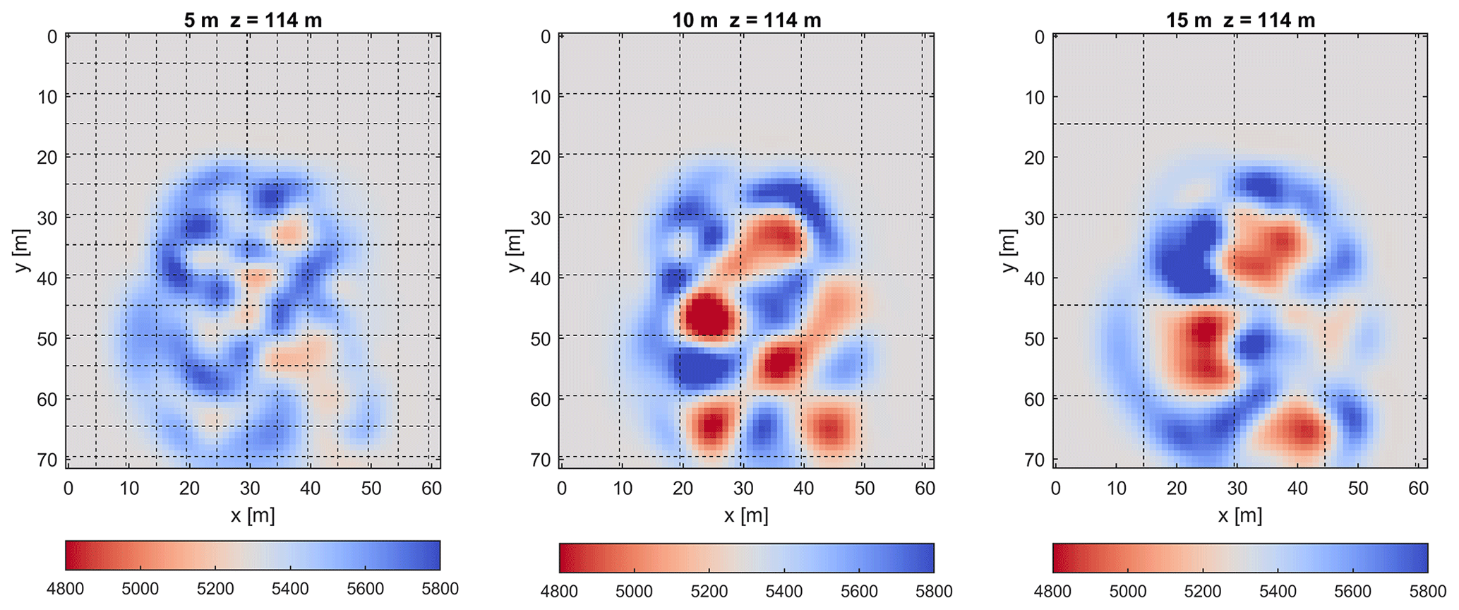
Figure A3 Horizontal cross section along a slice at z=114 m. The dashed lines indicate the locations and size of the checkerboard blocks. Block sizes are 5 (left), 10 (middle) and 15 (right) meters.