Statistical characteristics of non-volcanic tremor distributions along the Mexican Subduction Zone

We analyze the statistical characteristics of non-volcanic tremor (NVT) sequences in the Mexican subduction zone. To this end, we employ various techniques, including the Gutenberg–Richter relationship, non-extensive statistics, and multifractal detrended moving-average analysis, to extract information on magnitude and interevent-time distributions. The b-value results reveal that b ranges from 1.25 to 2.42, with the highest values occurring in the down-dip portion of the plate interface. In contrast, the q-value shows an inverse behavior, reaching its highest values in the interplate coupling region. Similar to tectonic earthquakes, NVT sequences exhibit a multifractal structure in both magnitude and interevent-time series. The multifractality analysis suggests that this behavior is associated with long-term correlations, the probability distribution of the data, and nonlinear dynamics. Both apparent and intrinsic multifractality are identified, with the former being dominant. Our estimates of the Hurst exponent (H) range from 0.65 to 1.06; most sequences indicate strong persistence (H>0.95), while values exceeding unity suggest a transition toward non-stationary behavior. These high temporal correlations may reflect localized fluid-perturbed regions, although this interpretation remains speculative. Regarding the distribution that best describes interevent sequences, we find that most sequences are well described by a Lognormal distribution and, to a lesser extent, by a Gamma distribution. Finally, observations of tectonic tremor duration exhibit substantial scatter, resulting in low coefficients of determination in scaling relationships. The source of this variability may be related to the NVT generation mechanism or to detection and characterization processes.

1 Introduction

Non-volcanic tremor (NVT) is an enigmatic seismic phenomenon that has become a topic of increasing interest, particularly in subduction zones. NVTs are emergent seismic signals of long duration and low amplitude (Obara, 2002). Previous studies have shown that NVTs are composed of repeating small low-frequency earthquakes, commonly accompanied by very-low-frequency earthquakes that, in both cases, involve shear failure and slip (Shelly et al., 2007; Bostock et al., 2015; Gomberg et al., 2016a, b). NVTs mainly occur along the plate interface, close to the shallow and deep edges of locked regions. This phenomenon can also be observed in other tectonic environments, such as in convergent margins (e.g., Taiwan; Tang et al., 2010) and continental transform faults (e.g., California; Nadeau and Dolenc, 2005; Shelly, 2010). Fluids are implicated in generating NVTs, similar to volcanic tremor processes (Obara, 2002). Pressure and temperature conditions in subduction zones, together with dehydration processes, control the occurrence of NVT (Yoshioka et al., 2008; Peacock, 2009). It has been reported that NVTs occur in regions of high pore-fluid pressure (Shelly et al., 2006). Other factors also contribute, including the composition of the overriding plate and processes such as metamorphism of subducting seamounts (Wada et al., 2008). Non-volcanic tremors commonly exhibit episodic activity, with periods of intense activity lasting from days to weeks, separated by quiescent intervals of months with few or no events (Obara, 2002). NVTs are also closely associated with slow earthquakes, with both phenomena sharing temporal and spatial occurrence (Rogers and Dragert, 2003). Another important feature of NVTs is their ability to be triggered by large earthquakes, such as the 2002 Denali earthquake (M_w=7.8) in Alaska (Rubinstein et al., 2007) and the 2003 Tokachi-oki earthquake (M_w=8.1) in Japan (Miyazawa and Mori, 2005), both of which triggered enhanced NVT activity.

Tectonic tremors have been reported along the Middle America Trench in Mexico, in the states of Guerrero (Payero et al., 2008; Cruz-Atienza et al., 2015; Villafuerte and Cruz-Atienza, 2017; Husker et al., 2019; Plata-Martínez et al., 2021; Chen et al., 2025), Jalisco-Colima (Ide, 2012), and Oaxaca (Brudzinski et al., 2010; Husker et al., 2019). In Guerrero, NVTs have been detected at approximately 200 km downdip, at depths of 40–50 km, and closer to the trench, at depths of 10–16 km (Plata-Martínez et al., 2021; Chen et al., 2025). Similarly, in Oaxaca, NVTs are located about 150–200 km from the trench at depths of 30–50 km (Brudzinski et al., 2010). In Western Mexico, NVTs occur in a narrow band oriented parallel to the trench, mostly at depths of 30–50 km (Ide, 2012). Much of the research on tectonic tremors has focused on locating events, generating catalogs, and their tectonic interpretation. Fewer studies, however, have examined the statistical characteristics of event occurrence. For example, Kao et al. (2010) determined the b-value of NVT sequences in northern Cascadia (M_w∼1.0–1.7), finding that the b-value of ∼1. Staudenmaier et al. (2019) estimated the b-value of NVTs in the San Andreas Fault ($\mathrm{0.44}<M_{\mathrm{w}}<\mathrm{2.7}$), obtaining a b-value of 2.52. In contrast, other studies reported extremely high b-values (b>5 with $\mathrm{1.5}<M_{\mathrm{w}}<\mathrm{2.7}$; b=4.2 with $\mathrm{0.3}<M_{\mathrm{w}}<\mathrm{1.5}$) (Sweet et al., 2014; Bostock et al., 2015). In this article, we studied the statistical features of NVT sequences generated at the Mexican subduction zone. We analyzed the Gutenberg-Richter relationship, non-extensive statistics, and multifractality of magnitude and interevent-time distributions. Our results provide detailed statistical characterization of NVTs in subduction zones, which may contribute to a better understanding of their generation mechanisms.

2 Tectonic setting

The Mexican subduction zone (MSZ) is located along the border of three tectonic plates: the Cocos (CO), North American (NA), and Rivera (RI) plates, respectively (Fig. 1). Convergence rates predicted from the NUVEL1-A model (DeMets et al., 1994) fluctuate from 2.0 to 6.8 cm yr⁻¹ for the RI-NA convergence in the north (Jalisco-Colima) to the CO-NA convergence in the south (Oaxaca), respectively (Fig. 1). The rupture areas of the previous largest earthquakes exhibit a seismic gap in the MSZ, known as the Guerrero seismic gap (GG). The GG is a 200 km long segment in the CO-NA plate boundary (Fig. 1). The gap is capable of producing an earthquake with a magnitude of 8.1–8.4 if the entire gap were ruptured in a single event (Singh and Mortera, 1991). The gap has not experienced a significant event (M>7) since 1911. The geometry of the subducted slab varies from north to south (Hayes et al., 2012). In the Jalisco region, the RI plate subducts at a steep angle (∼50°), and then the dip angle of the CO plate decreases gradually toward the southeast. In the Gurrero-Oaxaca region, the subducted slab is almost subhorizontal (Pardo and Suárez, 1995; Pérez-Campos et al., 2008). As mentioned above, non-volcanic tremors occur at certain regions within the subduction zone regime. They appear to signal the transition from creep to locking trench parallel segments (Chen et al., 2025).

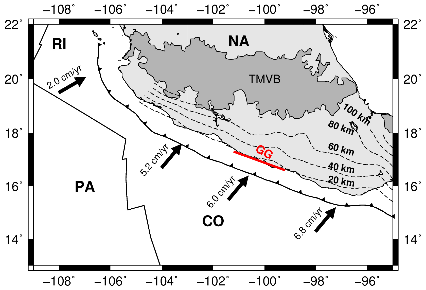
Figure 1 Tectonic framework of the Mexican subduction zone. TMVB is the Trans-Mexican Volcanic Belt. CO, NA, PA, and RI are the Cocos, North American, Pacific, and Rivera plates, respectively. GG is the Guerrero seismic gap. Black arrows indicate the convergence rate among tectonic plates. Dashed lines represent contour lines of the subducted plate, spaced every 20 km, from 20 to 100 km (Hayes et al., 2012).

3 Data and methods

3.1 Data

We retrieved non-volcanic tremor catalogs for six sequences along the Mexican subduction zone, as reported in previous studies (Ide, 2012; Idehara et al., 2014; Husker et al., 2019; Plata-Martínez et al., 2021; Chen et al., 2025). We studied NVT events occurring from 2005 to 2019 with hypocentral depths less than 50 km and magnitudes ranging from −0.8 to 3.65 (Table 1). Sequences 1, 3, and 4 occurred downdip of the coupling plate interface in the Guerrero segment, while sequences 5 and 6 took place at the coupling plate interface of the same segment. Sequence 2 was located further west, at the boundary between the subduction regimes of the Rivera and Cocos plates (Fig. 2). Catalogs for sequences 1–3 are available through the World Tremor Database (see the Data Availability section). The information reported in these catalogs includes origin time, hypocentral location, moment magnitude (M_w), and event duration for sequences 1–3 and 5. For sequence 4, locations were obtained using a single local seismic station, providing only origin time and hypocentral location. Similarly, sequence 6 does not report magnitudes. In this case, Chen et al. (2025) used an algorithm based on envelope correlation and matched filtering, providing location, duration, and average seismic energy rate instead of magnitude. Although magnitudes are unavailable for sequences 4 and 6, these catalogs provide sufficient information to analyze interevent times. Because NVTs often consist of superimposed low-frequency earthquakes (LFEs) of low amplitude, some studies prefer to use average energy or the root-mean-square (RMS) amplitude as a proxy for seismic energy. Hypocenters of NVTs were located in the states of Guerrero and Jalisco and were detected primarily using temporary seismic networks (sequences 1, 2, 3, 5, and 6). These networks include: the Mesoamerican Subduction Experiment (MASE, 2004–2007), Mapping the Rivera Subduction Zone (MARS, 2006–2007), and the Guerrero Seismic Gap project (G-GAP, 2009–2014).

Table 1 Studied non-volcanic tremor sequences. N is the number of events; M_w is the moment magnitude; T₁ and T₂ are the start and end dates of the located NVTs.

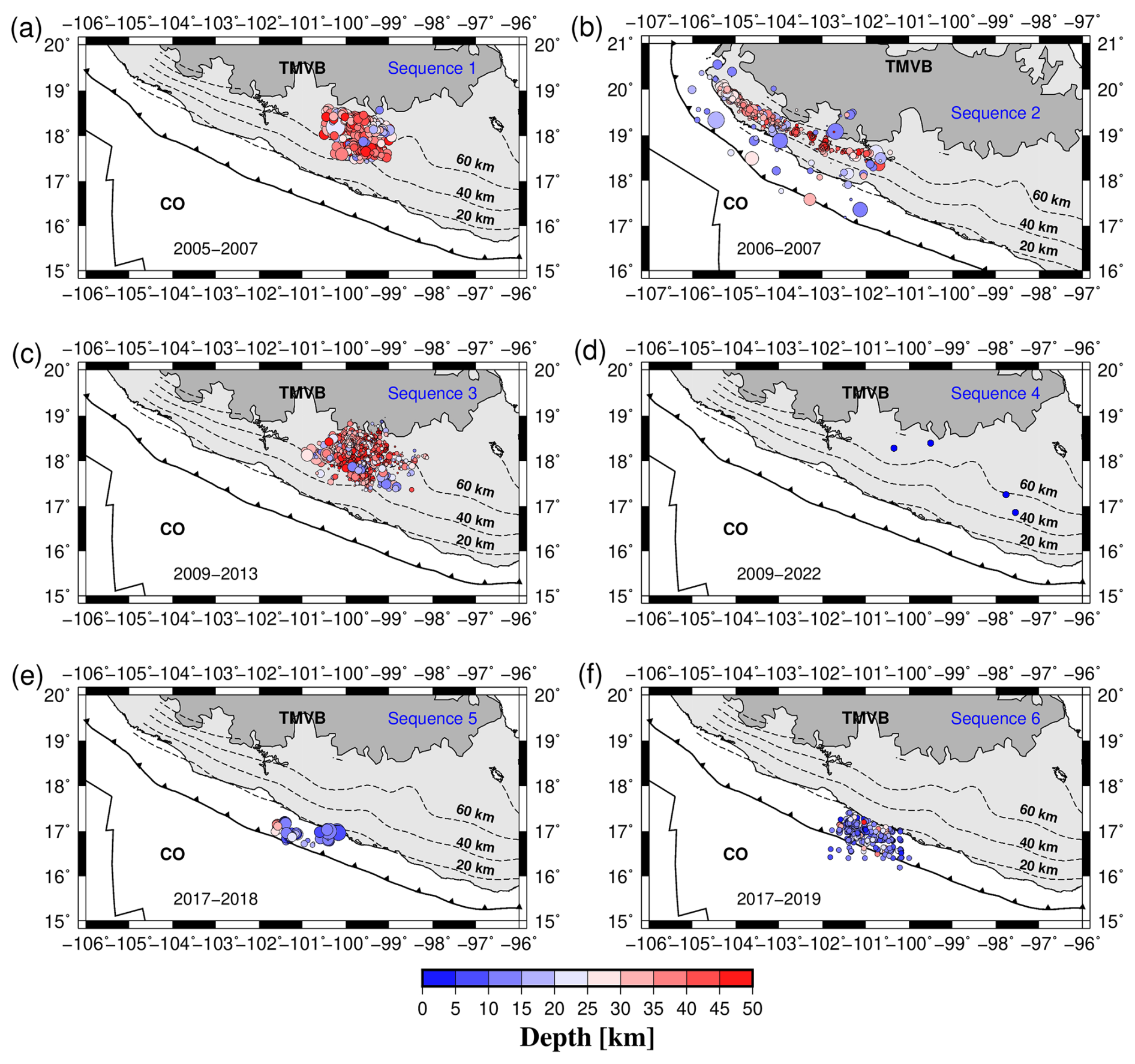
Figure 2 Hypocenter locations of all the studied non-volcanic tremor sequences along the Mexican subduction zone. (a) Sequence 1, (b) sequence 2, (c) sequence 3, (d) sequence 4, (e) sequence 5, and (f) sequence 6.

3.2 Methods

3.2.1 Estimation of the b-value

The earthquake frequency-magnitude distribution (FMD) is commonly described by the Gutenberg-Richter law (Gutenberg and Richter, 1944):

$$\begin{array}{}\text{(1)}& {\log }_{\mathrm{10}}N\left(M\right)=a+bM,\end{array}$$

where N is the number of earthquakes ≥M above the magnitude of completeness (M_c), a and b are constants that describe the earthquake productivity and the proportion of small to large events, respectively. Globally, the b-value is about one on average (Lay and Wallace, 1995). Fluctuations from this value are due to several factors, such as fluid pressure (Henderson et al., 1994), heterogeneity in the fault zone (Mogi, 1963), thermal gradient (Warren and Latham, 1970), and variations in the state of stress (Schorlemmer et al., 2005; Scholz, 2015). The b-value is determined using the maximum likelihood method proposed by Aki (1965). The equation that describes this estimator is the following

$$\begin{array}{}\text{(2)}& b={\displaystyle \frac{{\log }_{\mathrm{10}}e}{\stackrel{\mathrm{‾}}{M}-(M_{\mathrm{c}}-\mathrm{\Delta }M/\mathrm{2})}},\end{array}$$

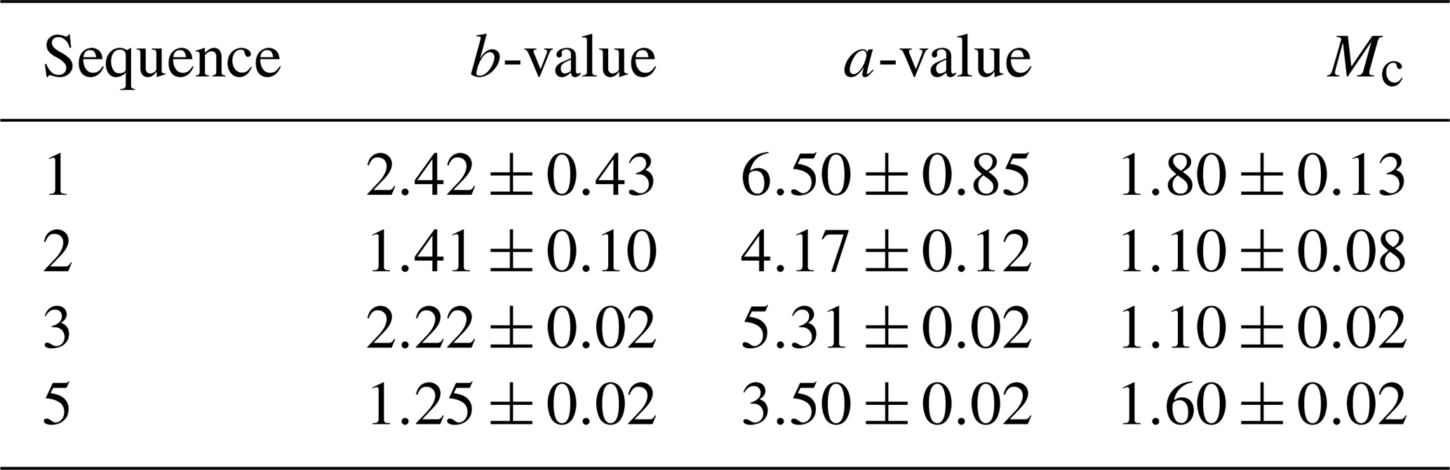
where M_c is the catalog completeness magnitude, $\stackrel{\mathrm{‾}}{M}$ is the average magnitude with a magnitude greater than M_c, and ΔM is the magnitude binning interval. M_c was estimated using the maximum curvature method (Woessner and Wiemer, 2005). We determined b-values for NVT sequences with reported magnitudes (sequences 1–3 and 5), and the results are shown in Fig. 3 and Table 2. Following Woessner and Wiemer (2005), we also used a bootstrap approach to estimate uncertainties in the b-value and M_c.

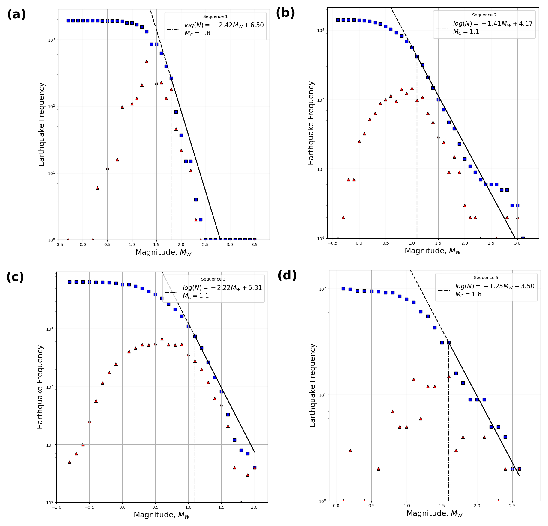
Figure 3 Estimates of b-value and M_c for the studied NVT sequences. Blue squares show the cumulative number of events versus magnitude. Red triangles exhibit the number of events. The solid black lines indicate the Gutenberg-Righter frequency magnitude distributions. (a) Sequence 1, (b) sequence 2, (c) sequence 3, and (d) sequence 5.

Table 2 Results for the Gutenberg-Richter relationship. Uncertainties were quantified based on a bootstrap approach.

3.2.2 Non-extensive statistical analysis

Non-extensive statistical mechanics (NESM) provides a theoretical framework for analyzing non-equilibrium complex systems, including earthquake phenomena. For systems exhibiting long-range correlations, memory effects, or fractal characteristics, NESM offers a particularly suitable mathematical approach (Tsallis, 2009). Within this context, Sotolongo-Costa and Posadas (2004) proposed the fragment asperity model, in which the release of seismic energy (ε) is linked to the size of r fragments that occupy the space between irregular fault interfaces. Silva et al. (2006) used a volumetric relationship between seismic energy and fragment size in the form of ε∝r³, under this assumption, the cumulative distribution of the number of earthquakes N with a magnitude greater than M is

$$\begin{array}{}\text{(3)}& \log {\displaystyle \frac{N>M}{N}}={\displaystyle \frac{(\mathrm{2}-q)}{(\mathrm{1}-q)}}\log \left[\mathrm{1}-\left({\displaystyle \frac{\mathrm{1}-q}{\mathrm{2}-q}}\right)\left({\displaystyle \frac{{\mathrm{10}}^{\mathrm{2}M}}{a_{\mathrm{s}}^{(\mathrm{2}/\mathrm{3})}}}\right)\right],\end{array}$$

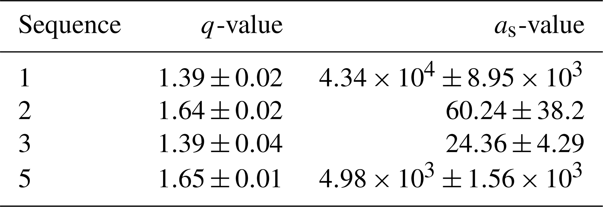
where the q-value is in the range of $\mathrm{1}<q<\mathrm{2}$, the constant a_s is a proportionality parameter between the released seismic energy and the fragment size. The q-value quantifies the length scale of spatial interactions; a q-value of ∼1 corresponds to short-range correlations, while increasing qindicates that the physical state becomes progressively more unstable. High q-values suggest that the fault planes are out of equilibrium, implying a higher likelihood of subsequent events (Sotolongo-Costa and Posadas, 2004). In most tectonic regimes, q typically ranges from 1.5 to 1.7 (Sarlis et al., 2010). We calculated the q-values for all NVT sequences with reported magnitudes. As in the case of b-values, we employed bootstrap resampling to quantify uncertainties in q. The results are presented in Fig. 4 and Table 3.

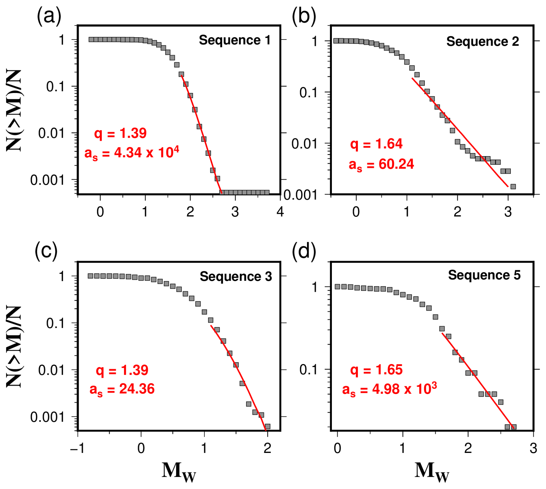
Figure 4 Normalized cumulative number of earthquake with magnitude m>M_th and fitting obtained with the fragment asperity model for the seismicity monitored in each NVT sequence. (a) Sequence 1, (b) sequence 2, (c) sequence 3, and (d) sequence 5.

Table 3 Results for the fragment asperity model. Uncertainties were quantified based on a bootstrap approach.

3.2.3 Multifractal detrended moving average analysis

The multifractal detrended fluctuation analysis (MFDFA) is a technique used to quantify the scaling behavior and correlations in time series (Kantelhardt et al., 2002). In seismology, MFDFA has shown that seismicity exhibits multifractal behavior, reflecting the nonlinear dynamics of tectonic processes (Telesca and Lapenna, 2006). The method has been applied to track the evolution of multifractal parameters across different stages of seismic activity (Monterrubio-Velasco et al., 2020) and in long-term regional studies (Alam et al., 2023), illustrating its ability to explore the organization and variability of seismic events. An improvement to MFDFA, the multifractal detrended moving average analysis (MFDMA), was proposed by Gu and Zhou (2010), providing enhanced robustness to trends and non-stationarities in the data. In this study, we employ MFDMA to investigate the multifractal properties of both interevent times and magnitude distributions of NVT sequences, allowing us to characterize apparent and intrinsic multifractality. We summarize the MFDMA algorithm of Gu and Zhou (2010) as follows. First, a cumulative time series of a given physical parameter D(t) is constructed and represented as

$$\begin{array}{}\text{(4)}& y\left(t\right)=\sum _{i=\mathrm{1}}^{t}D\left(i\right),\end{array}$$

where t=1, 2, 3, …, N (length of the time series) and D(i) is the observed time series. Then, a moving average function of y(t) is calculated in a moving window as

$$\begin{array}{}\text{(5)}& \stackrel{\mathrm{̃}}{y}={\displaystyle \frac{\mathrm{1}}{s}}\sum _{k=-\mathrm{1}\lfloor (s-\mathrm{1})\mathit{\theta }\rfloor }^{\lceil (s-\mathrm{1})(\mathrm{1}-\mathit{\theta })\rceil }y(t-k),\end{array}$$

where s is the window size. Here, ⌊x⌋ denotes the floor function (the largest integer less than or equal to x), while ⌈x⌉ represents the ceiling function (the smallest integer greater than or equal to x). The position parameter θ, describes the delay between the moving average function and the original time series ($\mathrm{0}<\mathit{\theta }<\mathrm{1}$). For example, if θ=0, 0.5, and 1, it describes a backward, centered, and forward moving average, respectively.

Afterwards, the residual sequences are obtained by detrending the time series through removing the average function, $\stackrel{\mathrm{̃}}{y}\left(i\right)$, resulting in

$$\begin{array}{}\text{(6)}& \mathit{ϵ}\left(i\right)=y\left(i\right)-\stackrel{\mathrm{̃}}{y}\left(i\right),\end{array}$$

where $s\le i\le N$. The residual series (ϵ(i)) is divided into N_s disjoint segments with the same size of s, where $N_{\mathrm{s}}=N/s-\mathrm{1}$. The residual sequence for each segment is denoted by ϵ_ν, where ${\mathit{ϵ}}_{\mathit{\nu }}\left(i\right)=\mathit{ϵ}(l+i)$ for $\mathrm{1}\le i\le s$ and $l=(\mathit{\nu }-\mathrm{1})s$. Then we calculate the root-mean-square fluctuation function (F_ν(s)) for a segment of size s as follows

$$\begin{array}{}\text{(7)}& F_{\mathit{\nu }}\left(s\right)={\left\{{\displaystyle \frac{\mathrm{1}}{s}}\sum _{i=\mathrm{1}}^s{\mathit{ϵ}}_{\mathit{\nu }}^{\mathrm{2}}\left(i\right)\right\}}^{\mathrm{1}/\mathrm{2}}.\end{array}$$

The qth order fluctuation function (F_q(s)) is obtained by

$$\begin{array}{}\text{(8)}& F_q\left(s\right)={\left\{{\displaystyle \frac{\mathrm{1}}{N_{\mathrm{s}}}}\sum _{\mathit{\nu }=\mathrm{1}}^{N_{\mathrm{s}}}{F}_{\mathit{\nu }}^q\left(s\right)\right\}}^{\mathrm{1}/q},\end{array}$$

for all q≠0. For the case of q=0, we have

$$\begin{array}{}\text{(9)}& \ln \left[F_{\mathrm{0}}\right(n\left)\right]={\displaystyle \frac{\mathrm{1}}{N_n}}\sum _{\mathit{\nu }=\mathrm{1}}^{N_{\mathrm{s}}}\ln \left[F_{\mathit{\nu }}\right(s\left)\right],\end{array}$$

where the scaling behavior of F_q(s) follows the relation that is given by F_q(s)∼s^h(q) where h(q) is the Holder exponent or generalized Hurst exponent. The multifractal scaling exponent is calculated by

$$\begin{array}{}\text{(10)}& \mathit{\tau }\left(q\right)=qh\left(q\right)-\mathrm{1}.\end{array}$$

Finally, the singularity strength function (α(q)) and the multifractal spectrum (f(α)) can be obtained as

$$\begin{array}{}\text{(11)}& \mathit{\alpha }\left(q\right)={\displaystyle \frac{\mathrm{d}\mathit{\tau }\left(q\right)}{\mathrm{d}q}},\end{array}$$

and

$$\begin{array}{}\text{(12)}& f\left(\mathit{\alpha }\right)=q\mathit{\alpha }-\mathit{\tau }\left(q\right),\end{array}$$

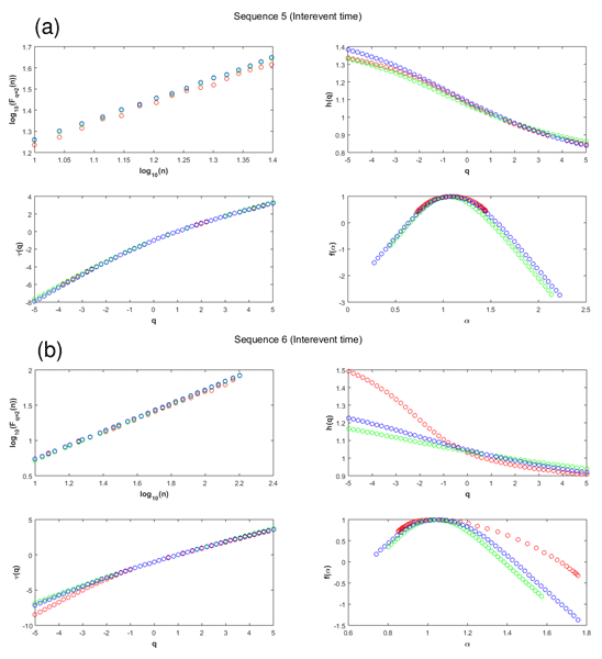
respectively. In the multifractal analysis of sequences 1 to 4, we used the following input parameters: N=30, θ=0, $q\in [-\mathrm{5},\mathrm{5}]$ with q increments of 0.2, the lower bound of segment size s is fixed to 10, while the upper bound is given by $N/\mathrm{10}$, as recommended by Gu and Zhou (2010). In the case of sequences 4 and 5, the upper bound of segment size s is set to $N/\mathrm{4}$ because they have less data than the other sequences. The parameters adopted ensure methodological consistency. The choice of N provides sufficient scale for local trend estimation, balancing statistical reliability in short series with detailed detrending in longer ones. θ=0 corresponds to a backward-moving average, preserving causality, while the q range probes multifractal behavior across fluctuation magnitudes and maintains numerical stability. This configuration enables robust, consistent scaling analysis across datasets of varying lengths. Results for F_q(s), h(q), τ(q), α(q), and f(α) for interevent time and magnitude distributions are shown in Figs. 5 and 6 and Figs. 7 to 9, respectively. In the MFDFA framework, q is the fluctuation order and is used to scan different fluctuation scales. In contrast, in the context of non-extensive statistical mechanics, the non-extensive parameter (q-value) quantifies non-additivity and entropy.

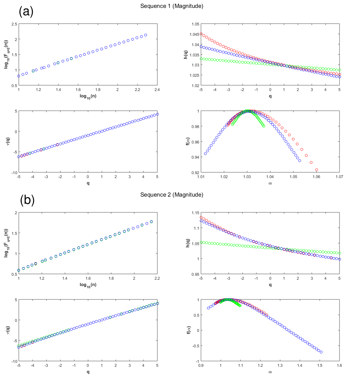
Figure 5 Multifractal analysis of magnitude for sequences 1 (a) and 2 (b) (fluctuation function, F(q); Hurst exponent, h(q); multifractal scaling exponent τ(q); and multifractal spectrum f(α)). In all cases, the original, shuffled, and IAAFT surrogates data are shown in red, green, and blue color, respectively.

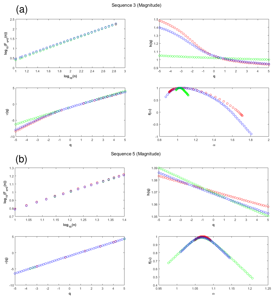
Figure 6 Multifractal analysis of magnitude for sequences 3 (a) and 5 (b) (fluctuation function, F(q); Hurst exponent, h(q); multifractal scaling exponent τ(q); and multifractal spectrum f(α)). In all cases, the original, shuffled, and IAAFT surrogates data are shown in red, green, and blue color, respectively.

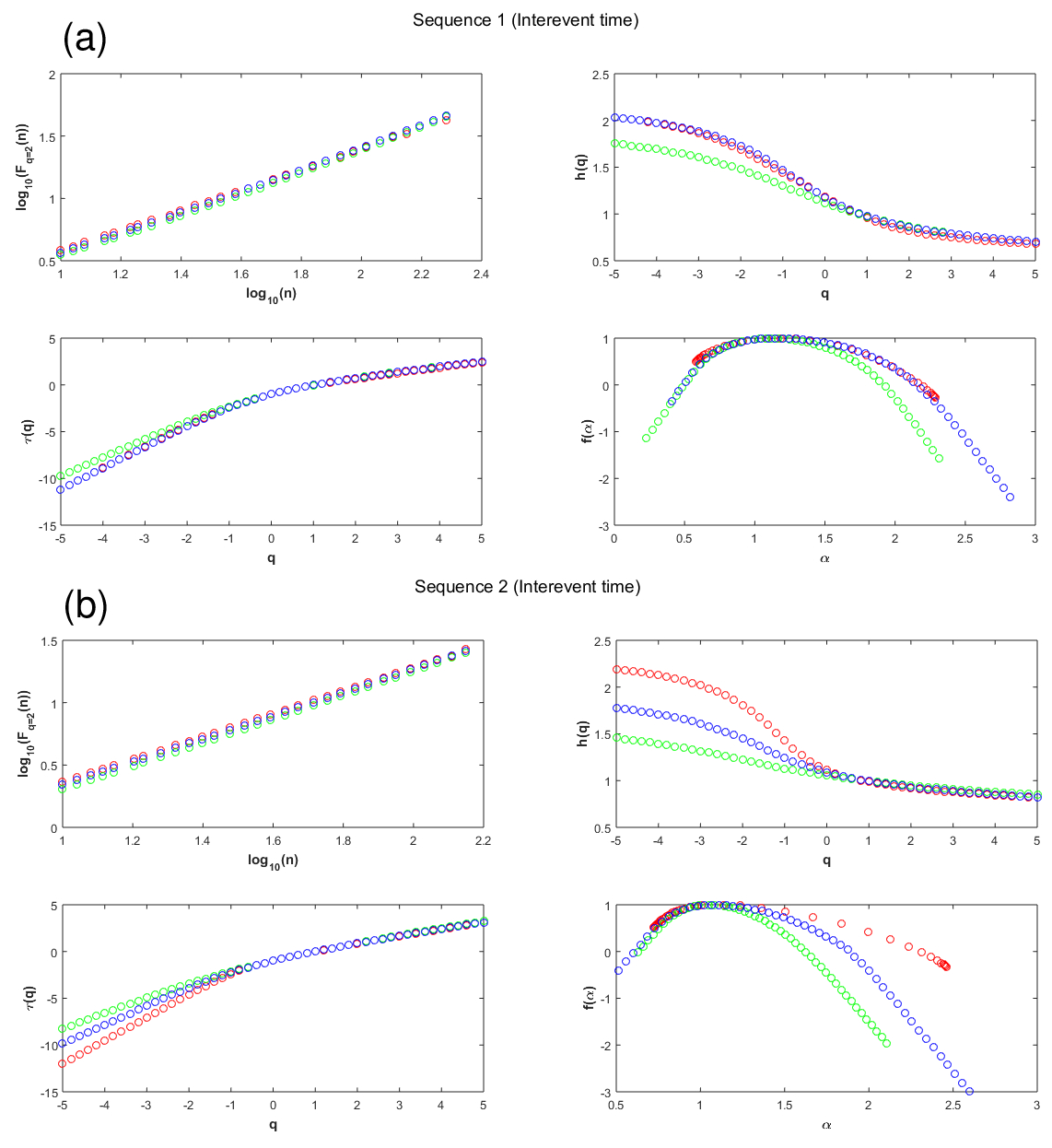
Figure 7 Multifractal analysis of interevent time for sequences 1 (a) and 2 (b) (fluctuation function, F(q); Hurst exponent, h(q); multifractal scaling exponent τ(q); and multifractal spectrum f(α)). In all cases, the original, shuffled, and IAAFT surrogates data are shown in red, green, and blue color, respectively.

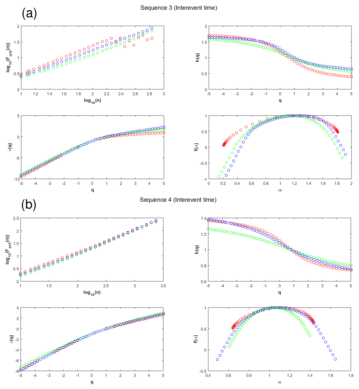
Figure 8 Multifractal analysis of interevent time for sequences 3 (a) and 4 (b) (fluctuation function, F(q); Hurst exponent, h(q); multifractal scaling exponent τ(q); and multifractal spectrum f(α)). In all cases, the original, shuffled, and IAAFT surrogates data are shown in red, green, and blue color, respectively.

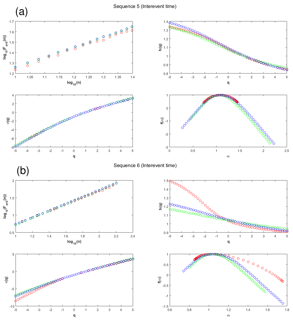
Figure 9 Multifractal analysis of interevent time for sequences 5 (a) and 6 (b) (fluctuation function, F(q); Hurst exponent, h(q); multifractal scaling exponent τ(q); and multifractal spectrum f(α)). In all cases, the original, shuffled, and IAAFT surrogates data are shown in red, green, and blue color, respectively.

3.2.4 Multifractal parameters

We determined multifractal parameters using the equations presented in the previous section, following De Freitas and França (2024). We start with the degree of asymmetry (A), defined as

$$\begin{array}{}\text{(13)}& A={\displaystyle \frac{{\mathit{\alpha }}_{\text{max}}-{\mathit{\alpha }}_{\mathrm{0}}}{{\mathit{\alpha }}_{\mathrm{0}}-{\mathit{\alpha }}_{\text{min}}}},\end{array}$$

where α₀ is the value for which f(α) is maximum. If A=1, f(α) is symmetric. On the contrary, when A>1, the symmetry is right-skewed, and if $\mathrm{0}<A<\mathrm{1}$, the symmetry is left-skewed. The values of α_max and α_min represent the extreme values of the singularity exponent and are related to the minimum and maximum fluctuation of the signal. The degree of multifractality (Δα), which is determined by

$$\begin{array}{}\text{(14)}& \mathrm{\Delta }\mathit{\alpha }={\mathit{\alpha }}_{\text{max}}-{\mathit{\alpha }}_{\text{min}}.\end{array}$$

A low value of Δα denotes that the time series is close to fractal. On the other hand, a high value of Δα indicates that the multifractal strength is higher (De Freitas and De Medeiros, 2009). The singularity parameter (Δf) describes the broadness of the singularity spectrum and is defined as

$$\begin{array}{}\text{(15)}& \mathrm{\Delta }f=f\left({\mathit{\alpha }}_{\text{max}}\right)-f\left({\mathit{\alpha }}_{\text{min}}\right).\end{array}$$

In the case that Δf>1, the left-hand side is less deep, while if Δf=0, both depths of the tails are equal. According to Ihlen (2012), a long left tail indicates that the singularities are stronger (many large fluctuations/more abrupt behavior). In contrast, a long right tail indicates that the singularities are weaker (smoother signal with smaller variations). The Hurst index (H) can be obtained from the multifractal spectrum through the second-order generalized Hurst exponent h(q=2). If H>0.5, it indicates persistence in long-range correlation, while H≈0.5 shows a random character of the series (past and future fluctuations are uncorrelated or Brownian motion). On the other hand, H<0.5 reflects anti-persistence. In this case, the fluctuations tend not to continue in the same direction, but instead turn back on themselves, resulting in a less smooth time series (Hampson and Mallen, 2011).

3.2.5 Sources of multifractality

Multifractality can be classified into two categories: apparent and intrinsic. The former type refers to the multifractality that arises from spurious or artifactual patterns, while the latter refers to a genuine origin derived from nonlinear processes within the data (Saichev and Sornette, 2006). The differentiation between apparent and intrinsic multifractality is crucial for understanding the underlying processes in a time series (Jiang et al., 2019). On the other hand, there are three primary sources for multifractality in time series: (1) the non-Gaussian distribution of innovations, (2) linear long-range correlations, and (3) nonlinear long-range correlations (Jiang et al., 2019; Wang et al., 2023). Two methods are commonly used to investigate these sources of multifractality: namely, the shuffling (Kantelhardt et al., 2002) and the surrogating (Theiler et al., 1992) procedures. These methods involve modifying the original sample to eliminate specific sources of multifractality. The first source (non-Gaussian distribution) is typically examined using shuffled time series. The random shuffling of a time series removes both linear and nonlinear temporal correlations (which may contribute to the scaling of F_q) while preserving the probability distribution (PDF) (Kantelhardt, 2009). Thus, if F_q from the shuffled series scales in the same way as that of the original series, one may infer that the scaling is primarily due to the probability distribution of the data. Conversely, if the shuffled series exhibits weaker multifractality compared to the original data, then multifractality likely arises from a combination of temporal correlations and the PDF. Consequently, if no multifractal features remain after performing the shuffling procedure, it can be interpreted that long-range correlations are the dominant source of multifractality in the original series.

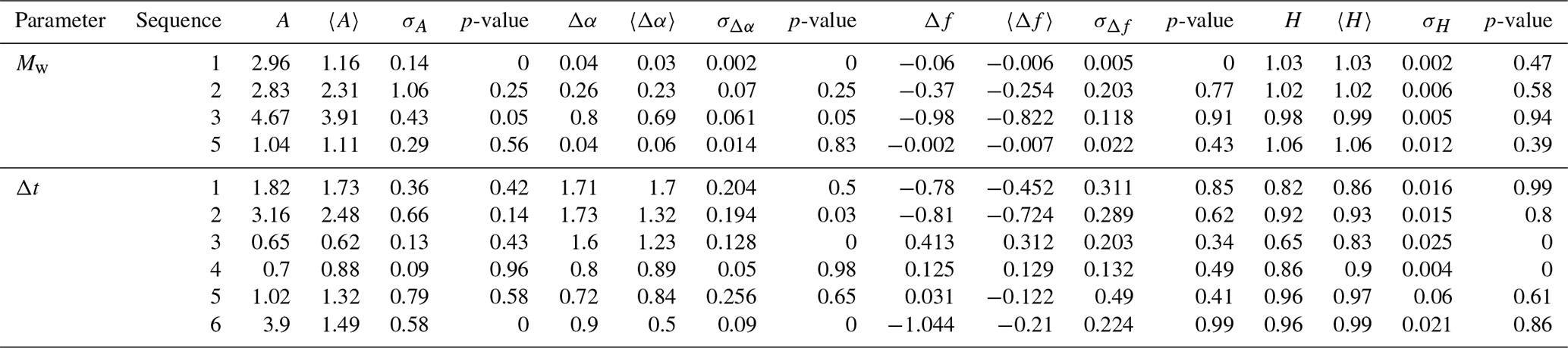
The surrogate time series method generates time series via a Fourier transform, preserving amplitudes while randomizing the phases, and then applying an inverse Fourier transform. In this form, non-linearities in the series are removed while preserving long-range correlations. The iterated amplitude-adjusted Fourier transform (IAAFT) algorithm (Schreiber and Schmitz, 1996, 2000) is appropriate for this purpose. Using the surrogate series, we performed statistical tests for h(q), τ(q), α(q), and f(α) to determine the presence or absence of intrinsic multifractality in the data. Specifically, the tests evaluate whether each indicator computed from the original series is greater than its counterpart derived from the IAAFT series. In other words, we calculate the probability that x is smaller than x_IAAFT ($p\text{-value}=\text{Pr}(x<x_{\text{IAAFT}})$), where x is a multifractal indicator, as proposed by Wang et al. (2023). Wang et al. (2023) also stated that if the p-value is smaller than a significance level (usually 5 %), then we can reject the hypothesis that the original time series is monofractal. Low p-values further suggest that the original time series exhibits intrinsic multifractality beyond fat-tailed distributions and linear long-range correlations. Alternatively, high p-values suggest the absence of intrinsic multifractality (De Freitas and França, 2024). Here, we applied MFDFA to the magnitude and interevent time series of NVT. In both cases, we generated 100 shuffled and IAAFT surrogate time series, and computed the multifractal indicators to analyze the source of multifractality. Surrogate data were used specifically used to assess the presence of intrinsic multifractality. The results are presented in Figs. 5 to 9 and Table 4.

Table 4 Testing multifractality of multifractal parameters. M_w is the moment magnitude; Δt is the interevent times; A is the degree of asymmetry; Δα is the degree of multifractality; Δf is the singularity parameter; and H is the Hurst index. The symbol 〈〉 denotes the mean and σ indicates the standard deviation. The p-values represent the proportion of IAAFT surrogates measured for each indicator that exceeds the index's value for the original time series.

3.2.6 Interevent-time distribution and duration scaling

Several interevent-time distributions have been proposed in the literature to explain earthquake interevent-time behavior (e.g., Gamma, Exponential, Lognormal, Weibull) (Corral, 2006; Davidsen and Kwiatek, 2013). We fitted interevent time data from all the NVT sequences, considering the previously mentioned statistical distributions, using the maximum likelihood estimation (MLE) method as described by Mesimeri et al. (2019). To determine the goodness of fit, we applied the Kolmogorov-Smirnov (KS) test. The Akaike and Bayesian information criteria (AIC and BIC, respectively) were also calculated to assess the relative quality of the statistical models. The best-fitting distribution is the one with the lowest AIC and BIC values. The obtained interevent-time probability distributions are shown in Fig. 10 and Table 5. Additionally, we determined scaling relationships between tremor duration and magnitude for sequences 1 to 3 and 5. The obtained scaling relations have the following form:

$$\begin{array}{}\text{(16)}& \log \left(\mathit{\tau }\right)=\mathit{\alpha }{M}_{\mathrm{w}}+\mathit{\beta },\end{array}$$

where τ is the duration of the NVT, M_w is the moment magnitude, and α and β are constants. We present the estimated scaling relationships in Fig. 11 and Table 5.

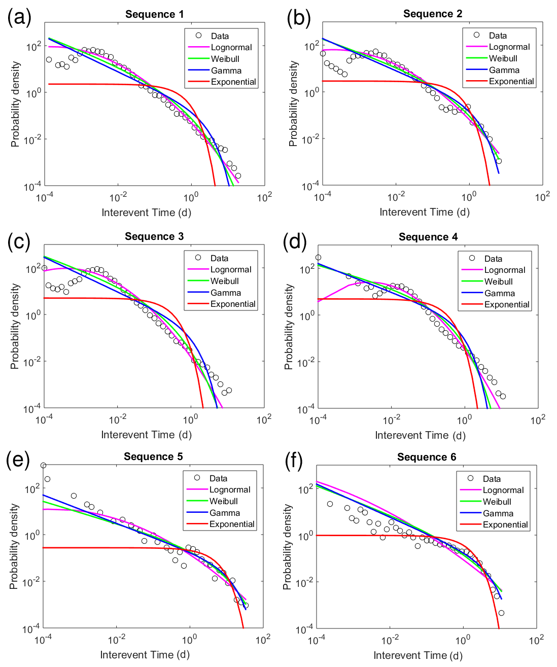
Figure 10 Probability density functions of the interevent times for the NVT sequences and fitted curves of different statistical distributions (exponential, Gamma, Lognormal, and Weibull). (a) Sequence 1, (b) sequence 2, (c) sequence 3, (d) sequence 4, (e) sequence 5, and (f) sequence 6.

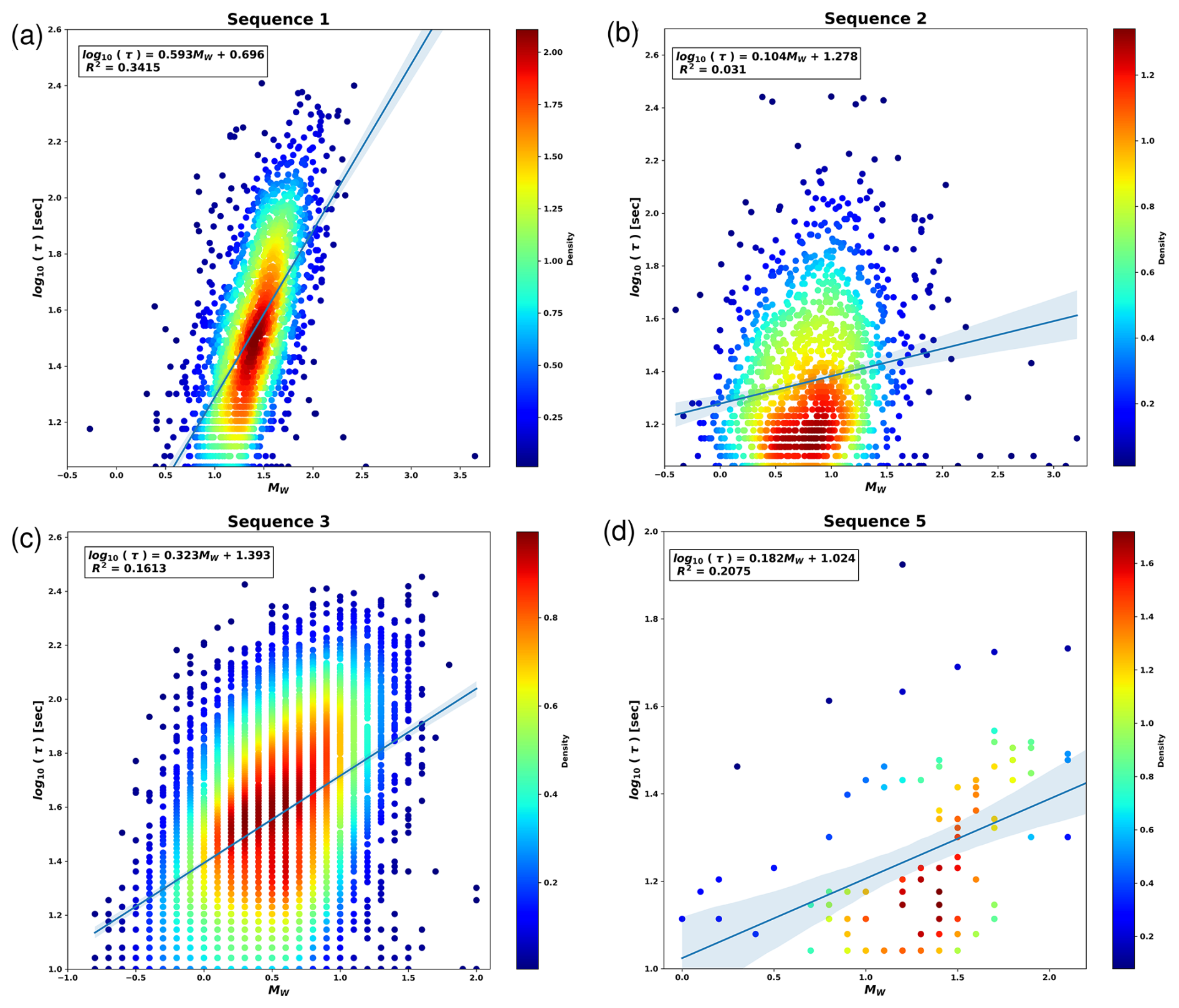
Figure 11 NVT duration scaling relationships (blue lines). In all figures, color indicates the density of NVT observations. (a) Sequence 1, (b) sequence 2, (c) sequence 3, and (d) sequence 5.

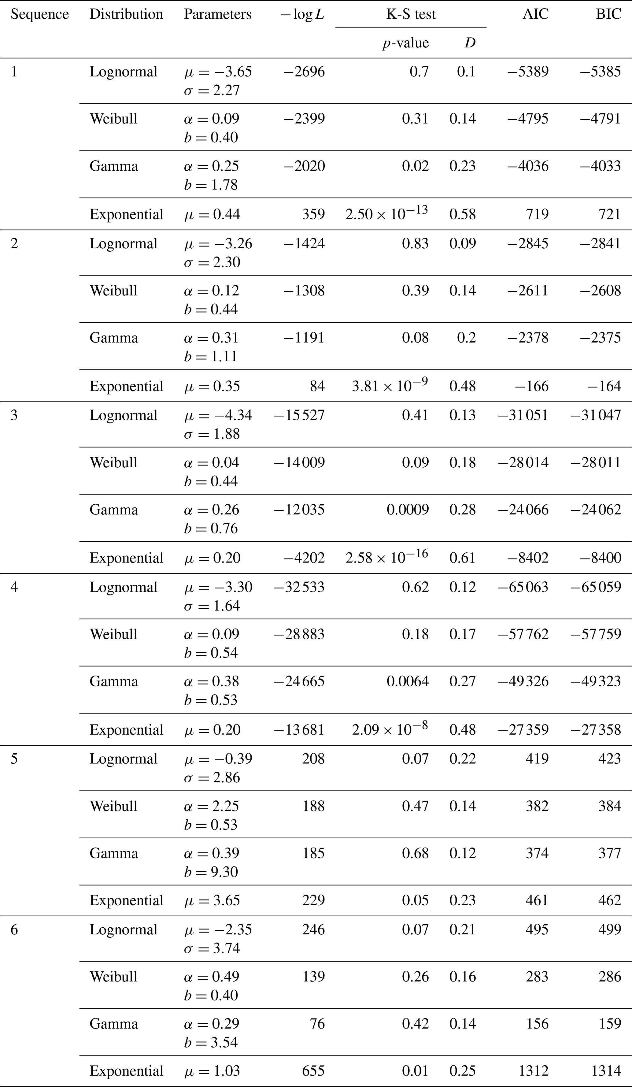
Table 5 Estimated parameters for the PDF of interevent times. AIC and BIC are the Akaike and Bayesian information criteria; D is the test statistic.

4 Results

Our estimates of the b-value showed that the b-values for NVTs at the Mexican subduction zone range from 1.25 to 2.42, with completeness magnitudes (M_c) between 1.10 and 1.80. Sequences 1 and 3 have the highest b-values, indicating a possible distinct characteristic of the down-dip Guerrero segment of the Cocos plate. They are followed by sequence 2, located at the interface between the Rivera and Cocos plates. The lowest b-value is found for sequence 5 in the Guerrero Gap region (Fig. 2 and Table 2), which unfortunately cannot be corroborated by sequence 6 at the same region, as it does not include magnitude data. The q-value from the non-extensive statistical analysis fluctuates from 1.39 to 1.65. The q-values show an apparent inverse relationship with the b-value, since the sequences located near the trench (2 and 5) have higher q-values than those located down-dip (1 and 3), which exhibit similar q-values. Bootstrap resampling (1000 iterations) was used to estimate uncertainties in b-values, M_c, and q-values (Tables 2 and 3). Smaller sequences (e.g., sequence 5, N=101) exhibit larger relative uncertainties, which are now explicitly reported. A Monte Carlo analysis incorporating these uncertainties confirms a strong negative correlation between b- and q-values, with mean Pearson coefficient $r=-\mathrm{0.94}$ (95 % CI: −0.999 to −0.743), supporting the inverse relationship observed across the NVT sequences.

Multifractal indicators of the original time series show that the multifractal spectra are mostly right-skewed (magnitude sequences 1 to 4, interevent time sequences 1, 2, and 6). In contrast, left-skewed spectra correspond to interevent time sequences 3 and 4. Sequence 5 exhibits a symmetric multifractal spectrum. Results for the degree of multifractality (Δα) indicate that interevent time series have a higher multifractal strength than magnitude time series. On the other hand, the singularity parameter (Δf) indicates that the singularities are weaker for magnitude sequences 2 and 3, as well as interevent time sequences 1–2 and 6. Conversely, the singularities are stronger for interevent time sequences 3 and 4. Estimates of the Hurst exponent (H) depict a long-term persistence signature (H>0.5). By comparing the multifractal spectra (Fq(s), h(q), τ(q), α(q), and f(α)) obtained from the original, shuffled, and surrogate time series, we observe that multifractality is not completely removed in all cases. However, in several sequences, the multifractal indicators become statistically indistinguishable from those derived from surrogate data. Statistical tests based on IAAFT surrogates show that p-values associated with the multifractal indicators (A, Δα, Δf, and H) vary significantly across sequences. Magnitude sequence 5 and interevent time sequences 1, 4, and 5 exhibit relatively high p-values, indicating no statistically significant differences with respect to surrogate data. In contrast, magnitude sequence 1 shows consistently low p-values across multiple indicators, suggesting statistically significant deviations from surrogate behavior. For the interevent time sequences 2, 3, and 6, low p-values are observed for key parameters, such as Δα, and, in sequence 3, for H as well, indicating significant differences relative to the surrogate series. In magnitude sequences 2 and 3, the results are mixed: some indicators yield low p-values, while others remain high, preventing a clear classification based solely on the statistical tests. Overall, the results indicate that the statistical significance of multifractality varies across sequences and depends on the specific indicator considered.

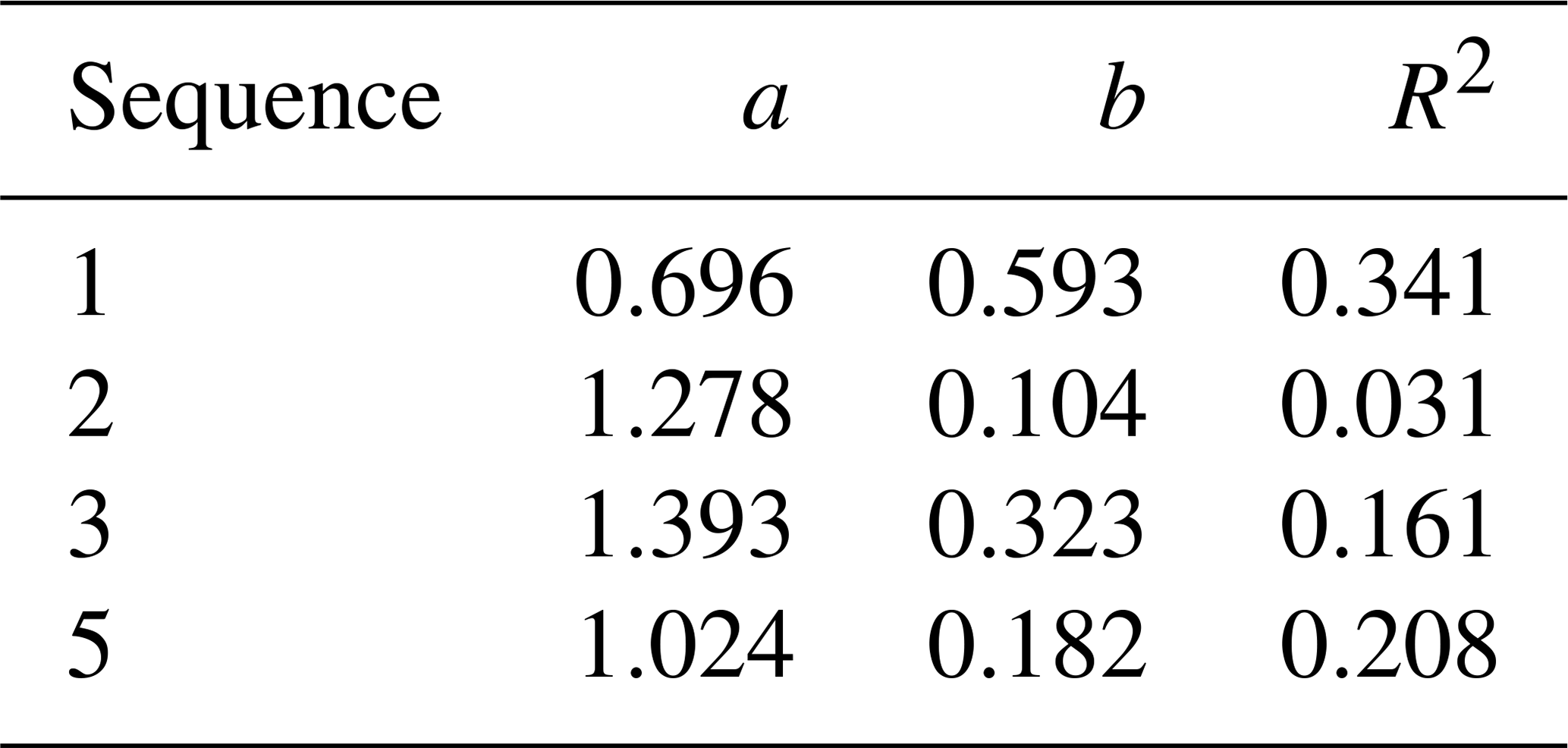
Regarding the inter-event time distributions, a comparison of the fitted probability density functions (PDFs) with the empirical distributions from sequences 1 to 4 showed that the Lognormal distribution provided the best fit. In contrast, for sequences 5 and 6, the Gamma distribution yielded the best fit for the interevent time data. In all cases, the least well-fitting distribution is the Exponential distribution (Fig. 10 and Table 5). Finally, event duration observations exhibit large scatter, resulting in linear scaling relationships with low coefficients of determination ($\mathrm{0.03}<R^{\mathrm{2}}<\mathrm{0.34}$) (Fig. 11 and Table 6). This scatter is intrinsic to the genesis of NVTs or is associated with the detection process, as it is present in all reported sequences.

Table 6 Duration scaling relationships ($\log \left(\mathit{\tau }\right)=a+b{M}_{\mathrm{w}}$). R² is the determination coefficient; b is the slope and a is the intercept.

5 Discussion

We start the discussion by comparing our b-value estimates with previous studies. The b-value associated with NVTs has been determined in both crustal and subduction environments, with the latter being the most common. In crustal regions, for example, along the San Andreas Fault (Parkfield segment), Staudenmaier et al. (2019) calculated a b-value of 2.52 for NVT episodes. For subduction zones, it has been found that the b-value of NVTs ranges between 1 and 5 (Kao et al., 2010; Rabbel et al., 2011; Gallego et al., 2013; Sweet et al., 2014; Bostock et al., 2015). The Cascadia subduction zone, particularly in Vancouver Island, exhibits both low and high b-values (b∼1 and $\mathrm{4.2}<b<\mathrm{5}$, respectively) (Kao et al., 2010; Sweet et al., 2014; Bostock et al., 2015). In Chile, the b-value of NVT sequences was determined to be 2.4 (Gallego et al., 2013). Regarding b-value estimations of NVTs at the Cocos plate, Rabbel et al. (2011) estimated a value of 1 in the region of Costa Rica. Our results show that the b-value varies from 1.25 to 2.42 for the NVTs detected in the Mexican subduction regime studied. We observed that in the down-dip segment, NVT sequences have the highest b-values (2.22–2.42), while in the interplate coupling region, the b-value ranges from 1.25 to 1.41 (Table 2). High b-values may indicate a greater degree of fracturing, as they reflect a larger proportion of small-magnitude events relative to larger ones. In general, the b-values obtained for the coupling region do not differ significantly from those reported for tectonic earthquakes. For example, for the Cocos plate, the b-value for tectonic seismic events has been observed to lie in the interval of 0.8–1.3 (Nishikawa and Ide, 2014).

Temporal variations in seismic network geometry can significantly influence the magnitude of completeness (M_c) for NVT sequences. Sequences 1–3 (Ide, 2012; Idehara et al., 2014) were recorded using temporary networks such as MARS and MASE, where changes in station coverage over time affected event detection and M_c estimates (N=1908, 1411, 6776; M_w ranges −0.27 to 3.65, −0.40 to 3.21, −0.80 to 2.00). Sequence 4 (Husker et al., 2019) was analyzed using limited station coverage, constraining the detection of low-magnitude events, although magnitudes were not estimated (N=23 408). In contrast, sequences 5 (Plata-Martínez et al., 2021) and 6 (Chen et al., 2025) used submarine seismometers, allowing reliable detection of events, despite Chen et al. (2025) not reporting magnitudes (N=101 and 637; M_w ranges 0.10 to 2.70 and not reported, respectively). These examples demonstrate that temporal changes in network configuration, station density, and instrument type may directly affect M_c and, consequently, influence b-value calculations and their interpretation for NVT catalogs.

In terms of the non-extensive statistical analysis, our estimates of the q-value for NVTs in Mexico are consistent with previous reports from subduction zones, where q-values range from 1.61 to 1.69 (Scherrer et al., 2015). These results agree with our findings, in which the q-value varies from 1.64 to 1.65. Our results also show that down-dip interplate sequences have lower q-values (1.39) (Table 3). High q-values in coastal regions may be explained by greater stress heterogeneity, associated with plate coupling and asperity distribution, compared to down-dip regions, where different conditions, such as pressure, temperature, and rock structure prevail.

Regarding the multifractal analysis, our results indicate that both magnitude and interevent time NVT sequences exhibit multifractal structures similar to those observed in tectonic earthquakes (interevent time, Michas et al., 2015; magnitude, De Freitas and França, 2024). Tests based on surrogate data show that only one sequence exhibits intrinsic multifractality, while four sequences display apparent multifractality and five sequences yield inconclusive results. De Freitas and França (2024) also reported that seismicity in some subduction zones shows apparent multifractality, whereas others exhibit intrinsic multifractality, which is consistent with our findings. The estimated Hurst exponent (H) values further illustrate the heterogeneity of the sequences, ranging from 0.65 to 1.06 (Table 4). Several sequences fall within the range typically associated with persistent behavior ($\mathrm{0.5}<H<\mathrm{1.0}$), while some sequences, including magnitude sequences 1, 2, and 5, reach or slightly exceed H=1.0. Values above unity should be interpreted with caution, as they may indicate non-stationary or trending behavior, rather than purely long-range dependence. Nonetheless, these high values may reflect strong temporal correlations in certain sequences.

High H values have previously been linked to fault-zone properties (Cisternas et al., 2004). While we hypothesize that they could reflect limited volumes of perturbed regions containing fluids, this interpretation remains speculative. The observed H values are statistically comparable to those reported for regional seismicity and aftershock sequences: southern Italy (0.5–0.92, Telesca et al., 2001), Taiwan and Greece (∼0.8, Chen et al., 2008; Gkarlaouni et al., 2017), and the San Andreas Fault (∼0.87, De Freitas et al., 2013), with Izmit aftershocks reaching 0.95 (Cisternas et al., 2004). Although fundamental differences exist between aftershock relaxation and NVT generation, the similarity in scaling behavior suggests comparable long-term memory in the underlying processes. The surrogate analysis indicates that the physical origin of multifractality is not uniform across sequences. Magnitude sequence 1 and interevent time sequences 2, 3, and 6 show statistically significant deviations from surrogate data, suggesting contributions from temporal correlations and potential nonlinear interactions, whereas other sequences are consistent with apparent multifractality arising from broad distributions or finite-size effects. Overall, these results support the interpretation that the observed multifractal behavior arises from a combination of mechanisms, whose relative influence varies across sequences and depends on their temporal organization.

The interevent time analysis showed that NVT sequences 1 to 4 are well described by a Lognormal distribution, while sequences 5 and 6 are better fitted by a Gamma distribution (Table 5). Although the Lognormal distribution provides the best fit for sequences 1 to 4, it can also occur in purely tectonic settings (Mesimeri et al., 2019), and thus its presence alone does not imply mixed tectonic-volcanic behavior. Our interpretation of “mixed behavior” is supported by additional indicators, including magnitude ranges, q-values, and variability in short- and long interevent times. Traversa and Grasso (2010) showed that a Gamma distribution mainly describes volcanic seismicity, although some episodes deviate from it, while purely tectonic activity can be captured by Exponential, Gamma, or Lognormal distributions (Corral, 2006; Passarelli et al., 2015; Post et al., 2021). Our results align with both global (M_w≥7, Bantidi, 2022) and regional ($\mathrm{0.1}<M_{\mathrm{l}}<\mathrm{5.1}$, Mesimeri et al., 2019) studies, where Lognormal distributions often provide the best description of interevent times. For sequences 5 and 6, the statistical preference for the Lognormal distribution is less clear, likely due to smaller sample sizes (Table 1), which increases uncertainty in the fits. Overall, the observed differences between down-dip and interplate coupling regions are consistent with this interpretation, with the Gamma distribution better explaining observations in the latter, likely reflecting the lower number of detected events.

Finally, the scaling relationship between tremor duration and magnitude for all NVT sequences exhibits substantial scatter. Although positive slope coefficients are consistently observed in $\log \left(\mathit{\tau }\right)=a+b{M}_{\mathrm{W}}$, the low coefficients of determination (R²=0.03–0.34) indicate a weak dependence of duration on magnitude, in contrast to the more robust scaling observed for regular earthquakes. Part of this variability may be related to observational limitations, as tremors lack clear phase arrivals and their parameters (e.g., duration, magnitude, and amplitudes) are more difficult to constrain (Staudenmaier et al., 2019). However, the persistence of this scatter across all sequences, despite similar tectonic settings and depths, suggests that it is not primarily controlled by first-order structural differences. Instead, this weak scaling likely reflects the complex and heterogeneous nature of tremor generation. Consistent with previous studies (Schwartz and Rokosky, 2007), this behavior suggests that tremor duration and magnitude may be governed by partially independent processes, highlighting that NVT does not follow simple earthquake-like scaling relationships. Although the relationship between slow earthquakes and tectonic tremors is not fully understood, there is evidence that NVTs are modulated by slow dislocations on the plate interface (Villafuerte and Cruz-Atienza, 2017).

6 Conclusions

We investigated the statistical features of reported NVT sequences along the Mexican subduction zone, analyzing the Gutenberg-Richter relation, non-extensive statistics, and multifractal behavior of magnitude and interevent time series. The estimated b-values range from 1.25 to 2.42, consistent with previous reports worldwide, with the highest values observed in down-dip regions. In contrast, q-values are lower in these regions compared to coastal areas ($\mathrm{1.39}<q<\mathrm{1.65}$), in agreement with the inverse relationship between b and q proposed in previous studies ($b=\mathrm{2}(\mathrm{2}-q)/(\mathrm{1}-q)$). Although quantitative differences exist, both approaches consistently indicate that higher b-values correspond to lower q-values. Both magnitude and interevent-time series exhibit multifractal behavior, similar to tectonic earthquakes. Our results show that the origin of this multifractality is not uniform across sequences, but rather arises from a combination of mechanisms whose relative importance varies. In several cases, the observed behavior is consistent with apparent multifractality associated with broad probability distributions, whereas in others, statistically significant deviations from surrogate data indicate contributions from long-range correlations and possible nonlinear dynamics. Overall, the results suggest that no single mechanism dominates and that the multifractal properties reflect the heterogeneous temporal organization of the sequences.

Most NVT sequences are well described by a Lognormal model, while a few are better fitted by a Gamma distribution. Although lognormal fits are common, they can also occur in purely tectonic settings; therefore, their presence alone does not imply mixed tectonic-volcanic behavior. Evidence from magnitude ranges, multifractal parameters, and interevent-time variability supports the interpretation of mixed statistical characteristics. These findings highlight the complex temporal patterns of NVT sequences and differences in clustering across regions. The relationship between tremor duration and magnitude, however, shows substantial scatter, resulting in weak scaling with low coefficients of determination. While positive scaling coefficients are consistently observed, their magnitudes remain poor predictors of tremor duration. Part of this variability may reflect observational uncertainties, as tremor signals lack clear phase arrivals and their parameters are difficult to constrain. Nevertheless, the persistence of this behavior across all sequences, despite similar tectonic settings and depths, suggests that first-order structural differences do not primarily control it. Rather, the weak correlation likely reflects the complex, heterogeneous nature of tremor generation, in which partially independent or multiscale processes may govern duration and magnitude.