Perturbation analysis of travel-time accuracy for core phases reconstructed from seismic interferometry

Correlating late coda waves from large earthquakes produces stable waveforms that approximate inter-station core phases. However, the properties of these coda waves often violate the strict assumptions underlying classical Green's function retrieval, undermining confidence in interpreting the reconstructed arrivals as true inter-station phases and limiting their utility in seismic imaging. In this study, we present a perturbation analysis of core-phase interferometry and show that accurate travel-time information can be recovered under locally uniform wave incidence along the inter-station path. We introduce a dimensionless parameter – defined as the ratio of the seismic wave period to the inter-station travel time – which establishes a critical angular threshold. Our perturbation analysis reveals that the travel-time reconstruction accuracy scales with the cube of this threshold, allowing high-precision recovery of core phases, which naturally exhibit small threshold values due to their long propagation paths. Numerical simulations validate the theoretical predictions. By applying the proposed framework to real coda correlation data, we demonstrate that core phases can be reliably reconstructed using a sufficiently large number of global earthquakes – even without the traditionally assumed uniform source distribution. These results establish a rigorous theoretical foundation for extracting high-precision core-phase travel times from coda correlations, enhancing the reliability of seismological imaging of Earth's deep interior.

1 Introduction

Over the past two decades, the use of ambient ground motions for imaging subsurface structures has advanced significantly. This progress is largely driven by the discovery that cross-correlating records between two stations yields waveforms with dispersion characteristics resembling those of surface waves propagating between them (Campillo and Paul, 2003; Snieder, 2004). Commonly used ambient seismic sources include microseisms (periods 1–50 s) and the Earth's hum (periods 50–300 s), both generated by interactions between ocean waves and the solid Earth (Hasselmann, 1963; Ardhuin et al., 2015), as well as high-frequency anthropogenic noise (periods <1 s). Dispersion measurements derived from ambient noise correlations have been extensively employed to probe Earth's interior structure (Shapiro et al., 2005; Sabra et al., 2005; Yao et al., 2006; Yang et al., 2007; Nishida et al., 2009; Wang et al., 2019).

Beyond ambient noise, late earthquake coda waves contain substantial body wave energy that has traversed deep Earth discontinuities. Consequently, coda correlations are enriched with core-sensitive phases that generally preserve accurate slowness information (Lin et al., 2013; Nishida, 2013; Boué et al., 2014; Wu et al., 2018). The travel times of these extracted phases have been utilized to constrain the fine-scale structure of the Earth's core (Wang et al., 2015; Costa de Lima et al., 2023; Phạm and Tkalčić, 2023).

Theoretically, the cross-correlation function (CCF) of noise records converges to the seismic Green's function under ideal conditions – such as a uniform distribution of noise sources enclosing the stations (Wapenaar, 2004) or equipartitioned wavefield energy (Lobkis and Weaver, 2001). However, coda waves often violate these ideal conditions, resulting in anomalously high amplitudes in reconstructed phases compared to earthquake data (Lin et al., 2013; Boué et al., 2014), as well as persistent features occurring at travel-time differences between conventional phases (Boué et al., 2014; Phạm et al., 2018; Kennett and Phạm, 2018a, b).

It is also well established that deviations from ideal conditions can introduce travel-time biases in wavefield reconstructions (Weaver et al., 2009; Tsai, 2009; Froment et al., 2010). As a result, it is widely recognized within the coda correlation community that core phases extracted from coda waves do not exactly represent the true inter-station core phases. Their travel times have been shown to be influenced by several factors, including earthquake–station geometry, focal mechanisms, and the specific coda time window selected for correlation. Previous studies have investigated the formation mechanisms of these phases under such variable conditions (Poli et al., 2017; Wang and Tkalčić, 2020b; Tkalčić et al., 2020).

This study aims to clarify under what realistic circumstances the travel times of coda-based core phases correspond to those of true inter-station arrivals. Such an evaluation is essential for assessing the reliability of using extracted travel times as substitutes for direct arrivals in imaging deep Earth structural anomalies. Previous theoretical treatments of noise correlations have often relied on asymptotic techniques – such as the stationary phase method – to derive approximate relationships, which inherently limits the rigor of travel-time accuracy assessments. To overcome this limitation, we introduce a perturbation-based framework to quantify potential travel-time discrepancies.

A key feature of this approach is the decomposition of the problem into a “solvable” reference model and a “perturbation” component. We begin with a bounded homogeneous model representing the solvable part, which is then perturbed to evaluate the accuracy of travel-time reconstruction. The proposed framework is validated through numerical simulations and further demonstrated using real coda correlation data.

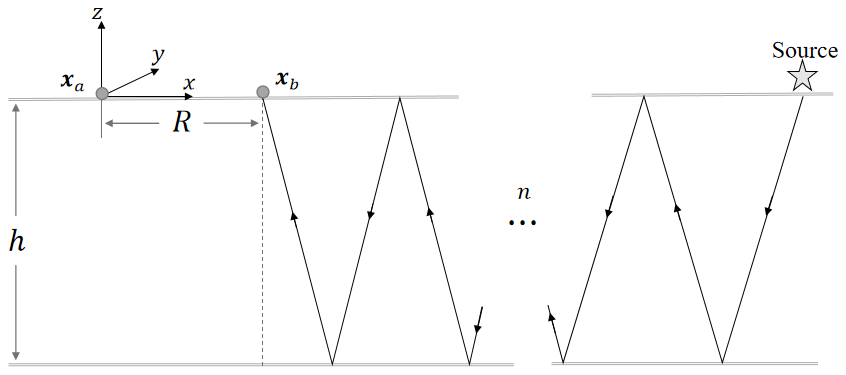
Figure 1 Definition of geometrical variables for wave propagation in the homogeneous medium bounded by two discontinuous layers.

2 Theory

2.1 A Solvable Reference Model

We consider a homogeneous medium bounded by two discontinuous surfaces to simulate wave reflections between the Earth's surface and the core–mantle boundary. The layer thickness is denoted by h. For simplicity, P–S wave conversion at the discontinuities is neglected, and the wave speed – whether for P or S waves – is represented by a constant c. Two seismic stations are positioned at ${\mathit{x}}_{\mathrm{a}}=(\mathrm{0},\mathrm{0},\mathrm{0})$ and ${\mathit{x}}_{\mathrm{b}}=(R,\mathrm{0},\mathrm{0})$, with all excitation sources placed within the surface layer (Fig. 1). For a wave originating from a source at position $\mathit{x}=(x,y,\mathrm{0})$ and undergoing m reflections from the lower boundary before reaching station x_a, the ray path length is given by:

$$\begin{array}{}\text{(1)}& r(\mathit{x},m)=\sqrt{x^{\mathrm{2}}+y^{\mathrm{2}}+\mathrm{4}{m}^{\mathrm{2}}{h}^{\mathrm{2}}}.\end{array}$$

Similarly, the path length for a wave arriving at x_b after experiencing n reflections is

$$\begin{array}{}\text{(2)}& r^{\prime }(\mathit{x},n)=\sqrt{(x-R{)}^{\mathrm{2}}+y^{\mathrm{2}}+\mathrm{4}{n}^{\mathrm{2}}{h}^{\mathrm{2}}}.\end{array}$$

For a wave traveling directly between the two stations after undergoing p reflections, the path length is:

$$\begin{array}{}\text{(3)}& L\left(p\right)=\sqrt{R^{\mathrm{2}}+\mathrm{4}{p}^{\mathrm{2}}{h}^{\mathrm{2}}}.\end{array}$$

The spectral representation of reflected waves recorded at either x_a or x_b, excited by a source located at x, can be expressed using a generalized ray formulation as:

$$\begin{array}{}\text{(4)}& \begin{array}{rl}{u}_i(\mathit{x},\mathit{\omega })=& {\mathrm{\Sigma }}_m{A}_i(\mathit{x},m,\mathit{\omega })e^{i\mathit{\omega }r(\mathit{x},m)/c}\\ u_j^{\prime }(\mathit{x};\mathit{\omega })=& {\mathrm{\Sigma }}_n{A}_j^{\prime }(\mathit{x},n,\mathit{\omega })e^{i\mathit{\omega }{r}^{\prime }(\mathit{x},n)/c}\end{array}.\end{array}$$

In these equations, ω represents the angular frequency, and i denotes the imaginary unit. The subscript i and j correspond to the three components of the displacement vector, respectively. The functions $A_i(\mathit{x},m,\mathit{\omega })$ and $A_j^{\prime }(\mathit{x},n,\mathit{\omega })$ represent the amplitude of reflected waves. In this study, we restrict our analysis to incident angles below the critical angle; consequently, neither $A_i(\mathit{x},m,\mathit{\omega })$ nor $A_j^{\prime }(\mathit{x},n,\mathit{\omega })$ incorporates a phase shift upon reflection and both remain real-valued.

In practical coda correlation analysis, researchers compute cross-correlations of late coda waves generated by individual earthquake events and subsequently stack the resulting CCFs for each station pair to enhance coherent arrivals. Following this procedure, the total CCF, summed over all sources, is theoretically expressed as:

$$\begin{array}{}\text{(5)}& \begin{array}{rl}{C}_{ij}\left(\mathit{\omega }\right)=& {\mathrm{\Sigma }}_s{u}_i^{*}(\mathit{x},\mathit{\omega })u_j^{\prime }(\mathit{x},\mathit{\omega })\\ =& {\mathrm{\Sigma }}_s{\mathrm{\Sigma }}_m{\mathrm{\Sigma }}_n{A}_i(\mathit{x},m,\mathit{\omega })A_j^{\prime }(\mathit{x},n,\mathit{\omega })e^{i\mathit{\omega }\mathit{\psi }(\mathit{x},m,n)},\end{array}\end{array}$$

where the summation over s corresponds to the contribution from all individual sources. The travel-time difference between the two ray paths is defined as:

$$\begin{array}{}\text{(6)}& \begin{array}{rl}\mathit{\psi }(\mathit{x},m,n)=& {\displaystyle \frac{r^{\prime }(\mathit{x},n)-r(\mathit{x},m)}{c}}\\ =& {\displaystyle \frac{\mathrm{1}}{c}}[\sqrt{(x-R{)}^{\mathrm{2}}+y^{\mathrm{2}}+\mathrm{4}{n}^{\mathrm{2}}{h}^{\mathrm{2}}}\\ & -\sqrt{x^{\mathrm{2}}+y^{\mathrm{2}}+\mathrm{4}{m}^{\mathrm{2}}{h}^{\mathrm{2}}}].\end{array}\end{array}$$

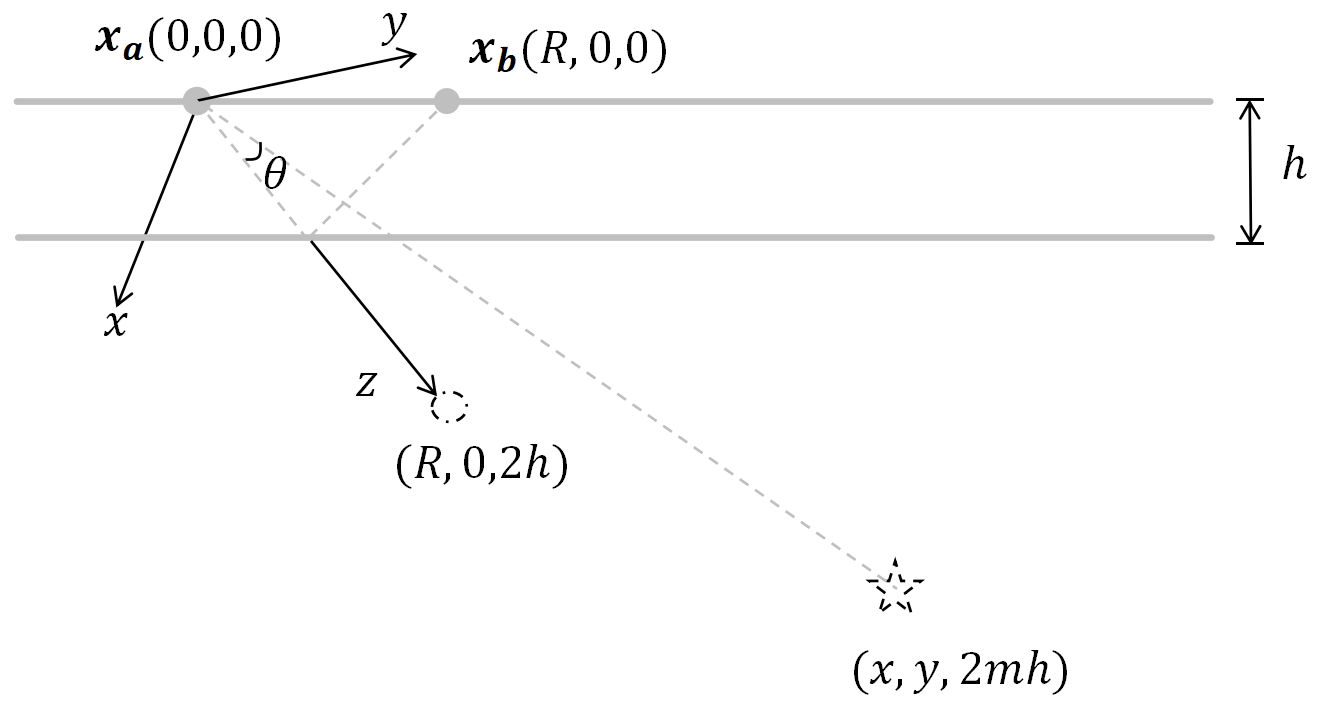
Figure 2 Definition of geometric variables for the case p=1. The dashed circle and star denote the station and source mapped from ${\mathit{x}}_{\mathrm{b}}=(R,\mathrm{0},\mathrm{0})$ and $(x,y,\mathrm{0})$, respectively.

2.2 Analytical Framework

The travel-time difference function in Eq. (6) corresponds to the difference in travel times for wave propagation in a homogeneous medium (Fig. 2). In this representation, the source is located at $(x,y,\mathrm{2}mh)$, and the two stations are positioned at $(\mathrm{0},\mathrm{0},\mathrm{0})$ and $(R,\mathrm{0},\mathrm{2}ph)$, where $p=m-n$. Based on this equivalence, we evaluate the CCF in Eq. (5) within this simplified homogeneous setting.

Since the cases p<0 and p>0 are complex conjugate in the computation, we consider only p>0 for simplicity. To facilitate the analysis, we apply a coordinate transformation by rotating the system about the y axis so that the z axis passes through the imaginary station at $(R,\mathrm{0},\mathrm{2}ph)$. In this rotated frame, we introduce spherical coordinates $(r,\mathit{\theta },\mathit{\varphi })$. Note that the z axis aligns with the reflected inter-station ray path originating from the station at $(\mathrm{0},\mathrm{0},\mathrm{0})$; thus, the polar angle θ represents the angular deviation of the incident wave from this ray path. Within this coordinate system, the travel-time difference function takes the form:

$$\begin{array}{}\text{(7)}& \begin{array}{rl}\mathit{\psi }(r,\mathit{\theta },\mathit{\varphi },p)=& {\displaystyle \frac{\mathrm{1}}{c}}\sqrt{(r\sin \mathit{\theta }\cos \mathit{\varphi }{)}^{\mathrm{2}}+(r\sin \mathit{\theta }\sin \mathit{\varphi }{)}^{\mathrm{2}}+[r\cos \mathit{\theta }-L(p){]}^{\mathrm{2}}}-{\displaystyle \frac{r}{c}}\\ =& {\displaystyle \frac{r}{c}}\sqrt{\mathrm{1}-{\displaystyle \frac{\mathrm{2}L\left(p\right)\cos \mathit{\theta }}{r}}+{\displaystyle \frac{L(p{)}^{\mathrm{2}}}{r^{\mathrm{2}}}}}-{\displaystyle \frac{r}{c}}\\ =& -{\displaystyle \frac{L\left(p\right)}{c}}\cos \mathit{\theta }\end{array}.\end{array}$$

The final approximation holds under the condition r>>L(p), which corresponds to m>>p.

In the CCF Eq. (5), the variable pair (x,m) can be mapped to the spherical coordinates $(r,\mathit{\theta },\mathit{\varphi })$, and similarly, (x,n) corresponds to $(r,\mathit{\theta },\mathit{\varphi },p)$. To proceed, we introduce a continuous function $\mathit{\eta }(r,\mathit{\theta },\mathit{\varphi })$ to represent the density of the source distribution, which encapsulates the discrete contributions governed by the indices s and m. This allows the double summation over s and m to be approximated by a volume integral. Accordingly, the CCF can be rewritten as:

$$\begin{array}{}\text{(8)}& \begin{array}{rl}{C}_{ij}\left(\mathit{\omega }\right)& ={\mathrm{\Sigma }}_s{\mathrm{\Sigma }}_m{\mathrm{\Sigma }}_p{A}_i(r,\mathit{\theta },\mathit{\varphi },\mathit{\omega })A_j^{\prime }(r,\mathit{\theta },\mathit{\varphi },p,\mathit{\omega })e^{i\mathit{\omega }\mathit{\psi }(r,\mathit{\theta },\mathit{\varphi })}\\ & ={\mathrm{\Sigma }}_p\underset{\mathrm{0}}{\overset{\mathit{\pi }/\mathrm{2}}{\int }}\underset{\mathrm{0}}{\overset{\mathrm{2}\mathit{\pi }}{\int }}{S}_{ij}(\mathit{\theta },\mathit{\varphi },p,\mathit{\omega })e^{-ikL\left(p\right)\cos \mathit{\theta }}\sin \mathit{\theta }\mathrm{d}\mathit{\theta }\mathrm{d}\mathit{\varphi },\end{array}\end{array}$$

where $k=\mathit{\omega }/c$ is the wavenumber, and

$$\begin{array}{}\text{(9)}& S_{ij}(\mathit{\theta },\mathit{\varphi },p,\mathit{\omega })=\underset{r_{\mathrm{1}}}{\overset{r_{\mathrm{2}}}{\int }}\mathit{\eta }(r,\mathit{\theta },\mathit{\varphi })A_i(r,\mathit{\theta },\mathit{\varphi },\mathit{\omega })A_j^{\prime }(r,\mathit{\theta },\mathit{\varphi },p,\mathit{\omega })r^{\mathrm{2}}\mathrm{d}r.\end{array}$$

In the function $S_{ij}(\mathit{\theta },\mathit{\varphi },p,\mathit{\omega })$, we assume that the wave amplitudes at the two stations maintain a constant proportionality when excited by different sources. Under this assumption, $S_{ij}(\mathit{\theta },\mathit{\varphi },p,\mathit{\omega })$ represents the wave energy density within each solid angle. We further assume that this energy density is uniform across all solid angles and denote it as ${\overline{S}}_{ij}(p,\mathit{\omega })$. Consequently, the CCF can be expressed as:

$$\begin{array}{}\text{(10)}& \begin{array}{rl}{C}_{ij}\left(\mathit{\omega }\right)=& {\mathrm{\Sigma }}_p\mathrm{2}\mathit{\pi }{\overline{S}}_{ij}(p,\mathit{\omega }){\displaystyle \frac{e^{-ikL\left(p\right)\cos \mathit{\theta }}}{ikL\left(p\right)}}{|}_{\mathrm{0}}^{{\mathit{\theta }}_{\mathrm{0}}}\\ =& \mathrm{2}\mathit{\pi }c{\mathrm{\Sigma }}_p{\overline{S}}_{ij}(p,\mathit{\omega })\mathit{\left\{}\right[{\displaystyle \frac{e^{ikL\left(p\right)}}{i\mathit{\omega }L\left(p\right)}}{]}^{*}\\ & -\left[{\displaystyle \frac{e^{ikL\left(p\right)\cos {\mathit{\theta }}_{\mathrm{0}}}}{i\mathit{\omega }L\left(p\right)}}{]}^{*}\mathit{\right\}}.\end{array}\end{array}$$

Here, θ₀ represents upper boundary of the polar angle. We assume it is azimuthally symmetric (independent of ϕ). In the time domain, the first term of this equation corresponds to arrivals at the travel times of the reflected waves between the two stations, where the factor $\mathrm{1}/i\mathit{\omega }$ corresponds to a time-domain integration operator. The second term corresponds to spurious waves arising due to a uniform truncation of the polar angle at different azimuthal angles. When p<0, we consider the complex conjugate of the CCF expression in Eq. (5). Following the same derivation, we obtain an equivalent expression. As a result, these arrivals appear on the causal and anti-causal sides of the CCF, respectively.

To ensure accurate reconstruction of the reflected waves, the polar angle θ₀ must be sufficiently large to prevent interference from spurious waves. This condition is met when the arrival times of the reflected and spurious wave packets are separated by at least one dominant period, corresponding to a 2π phase difference in the spectral domain. Adopting this phase difference as our non-interference criterion, we obtain the inequality:

$$\begin{array}{}\text{(11)}& kL\left(p\right)-kL\left(p\right)\cos {\mathit{\theta }}_{\mathrm{0}}\ge \mathrm{2}\mathit{\pi }.\end{array}$$

This yields a threshold angle expression:

$$\begin{array}{}\text{(12)}& {\mathit{\theta }}_{\mathrm{0}}=\mathrm{2}\arcsin \sqrt{{\displaystyle \frac{\mathit{\lambda }}{\mathrm{2}L\left(p\right)}}}\text{i.e.,}{\mathit{\theta }}_{\mathrm{0}}=\mathrm{2}\arcsin \sqrt{{\displaystyle \frac{T}{\mathrm{2}t\left(p\right)}}}.\end{array}$$

Here, T is the period of the reflected wave, and t(p) denotes the travel time of the inter-station wave after p reflections. To ensure accurate wave reconstruction, this result defines the minimum angular range required for locally uniform illumination.

2.3 Perturbation Analysis for Realistic Coda Correlations

The derivation above assumes a cosine distribution for the travel time difference function, which depends on wave propagation taking place within a bounded homogeneous medium. In practice, this condition is not satisfied. Furthermore, late earthquake coda correlations also involve P-to-S wave conversions. Under these circumstances, the actual travel time difference function deviates from the cosine form. To accommodate such deviations, we express the perturbed travel time differences as:

$$\begin{array}{}\text{(13)}& \mathit{\psi }(r,\mathit{\theta },\mathit{\varphi },p)=-t\left(p\right)\cos \mathit{\theta }+\mathit{\delta }(\mathit{\theta },p),\end{array}$$

where t(p) now represents the travel time along curved ray paths between the two stations after p reflections, θ is the polar angle between the incident wave direction and the z axis (where the z axis is aligned with the direction of the inter-station wave incidence at the station), and δ(θ,p) captures deviations from the idealized cosine distribution. Our analysis assumes azimuthal symmetry (i.e., independent of ϕ) and ignores the dependence on travel distance r for simplicity. The formalism can be readily extended to incorporate such dependencies by performing the analysis over discrete values of ϕ and r.

Since θ=0 corresponds to the inter-station ray path, the travel time difference at this angle attains its extreme value. We impose:

$$\begin{array}{}\text{(14)}& \mathit{\delta }(\mathrm{0},p)=\mathrm{0}\text{ and }{\mathit{\delta }}^{\left(\mathrm{1}\right)}(\mathrm{0},p)=\mathrm{0},\end{array}$$

where the superscript (n) denotes the nth derivative with respect to θ. Expanding δ(θ,p) in a Taylor series around θ=0, the travel time difference becomes:

$$\begin{array}{}\text{(15)}& \begin{array}{rl}\mathit{\psi }(r,\mathit{\theta },\mathit{\varphi },p)=& -t\left(p\right)\cos \mathit{\theta }+{\displaystyle \frac{\mathrm{1}}{\mathrm{2}}}{\mathit{\delta }}^{\left(\mathrm{2}\right)}(\mathrm{0},p){\mathit{\theta }}^{\mathrm{2}}\\ & +{\displaystyle \frac{\mathrm{1}}{\mathrm{6}}}{\mathit{\delta }}^{\left(\mathrm{3}\right)}(\mathrm{0},p){\mathit{\theta }}^{\mathrm{3}}+{\displaystyle \frac{\mathrm{1}}{\mathrm{24}}}{\mathit{\delta }}^{\left(\mathrm{4}\right)}(\mathrm{0},p){\mathit{\theta }}^{\mathrm{4}}+\mathrm{\cdots }\\ =& {\mathit{\delta }}^{\left(\mathrm{2}\right)}(\mathrm{0},p)-\left[{\mathit{\delta }}^{\left(\mathrm{2}\right)}\right(\mathrm{0},p)+t(p\left)\right]\cos \mathit{\theta }\\ & +{\displaystyle \frac{\mathrm{1}}{\mathrm{6}}}{\mathit{\delta }}^{\left(\mathrm{3}\right)}(\mathrm{0},p){\mathit{\theta }}^{\mathrm{3}}+{\displaystyle \frac{\mathrm{1}}{\mathrm{24}}}\left[{\mathit{\delta }}^{\left(\mathrm{2}\right)}\right(\mathrm{0},p)\\ & +{\mathit{\delta }}^{\left(\mathrm{4}\right)}(\mathrm{0},p)]{\mathit{\theta }}^{\mathrm{4}}+\mathrm{\cdots },\end{array}\end{array}$$

where the second line follows from substituting the Taylor expansion of cos θ.

Truncating the series at the θ³ term and substitute into Eq. (8) (assuming that the polar angle is truncated at θ₀, beyond which wave construction is not affected) yields:

$$\begin{array}{}\text{(16)}& \begin{array}{rl}{C}_{ij}\left(\mathit{\omega }\right)=& {\mathrm{\Sigma }}_p\underset{\mathrm{0}}{\overset{{\mathit{\theta }}_{\mathrm{0}}}{\int }}\underset{\mathrm{0}}{\overset{\mathrm{2}\mathit{\pi }}{\int }}{S}_{ij}(p,\mathit{\omega })e^{i\mathit{\omega }\mathit{\left\{}{\mathit{\delta }}^{\left(\mathrm{2}\right)}\right(\mathrm{0},p)-[{\mathit{\delta }}^{\left(\mathrm{2}\right)}(\mathrm{0},p)+t\left(p\right)\left]\cos \mathit{\theta }\mathit{\right\}}}\sin \mathit{\theta }d\mathit{\theta }d\mathit{\varphi }\\ =& {\mathrm{\Sigma }}_p{\displaystyle \frac{\mathrm{2}\mathit{\pi }{S}_{ij}(p,\mathit{\omega })}{i\mathit{\omega }\left[{\mathit{\delta }}^{\left(\mathrm{2}\right)}\right(\mathrm{0},p)+t(p\left)\right]}}{e}^{i\mathit{\omega }{\mathit{\delta }}^{\left(\mathrm{2}\right)}(\mathrm{0},p)}\cdot e^{-i\mathit{\omega }\left[{\mathit{\delta }}^{\left(\mathrm{2}\right)}\right(\mathrm{0},p)+t(p\left)\right]\cos \mathit{\theta }}{|}_{\mathrm{0}}^{{\mathit{\theta }}_{\mathrm{0}}}\\ =& {\mathrm{\Sigma }}_p{\displaystyle \frac{\mathrm{2}\mathit{\pi }{S}_{ij}(p,\mathit{\omega })}{{\mathit{\delta }}^{\left(\mathrm{2}\right)}(r,\mathrm{0},p)+t\left(p\right)}}\mathit{\{}{\displaystyle \frac{e^{i\mathit{\omega }\left[{\mathit{\delta }}^{\left(\mathrm{2}\right)}\right(\mathrm{0},p\left)\right(\mathrm{1}-\cos {\mathit{\theta }}_{\mathrm{0}})-t(p\left)\cos {\mathit{\theta }}_{\mathrm{0}}\right]}}{i\mathit{\omega }}}\\ & +\left[{\displaystyle \frac{e^{i\mathit{\omega }t\left(p\right)}}{i\mathit{\omega }}}{]}^{*}\mathit{\right\}}.\end{array}\end{array}$$

This result shows that the correlation still yields waves at the travel times of the reflected waves when truncating the series of the deviation function δ(θ,p) at θ³. We adopt, as before, our non-interference criterion for the phase difference. This leads to the condition:

$$\begin{array}{}\text{(17)}& \mathit{\omega }t\left(p\right)+\mathit{\omega }\left[{\mathit{\delta }}^{\left(\mathrm{2}\right)}\right(\mathrm{0},p\left)\right(\mathrm{1}-\cos {\mathit{\theta }}_{\mathrm{0}})-t(p\left)\cos {\mathit{\theta }}_{\mathrm{0}}\right]\ge \mathrm{2}\mathit{\pi }.\end{array}$$

We obtain a threshold angle expression:

$$\begin{array}{}\text{(18)}& {\mathit{\theta }}_{\mathrm{0}}=\mathrm{2}\arcsin \sqrt{{\displaystyle \frac{T}{\mathrm{2}\left[t\right(p)+{\mathit{\delta }}^{\left(\mathrm{2}\right)}(\mathrm{0},p\left)\right]}}},\end{array}$$

The second derivative ${\mathit{\delta }}^{\left(\mathrm{2}\right)}(r,\mathrm{0},p)$ affects the polar angle range over which the wavefield needs to be locally uniform. If we neglect its impact in this equality, the expression reduces to equality (12).

Equation (16) demonstrates that time errors due to deviations from the cosine distribution arise from higher-order terms (θ³ and beyond) in the Taylor series expansion of the travel time difference function $\mathit{\psi }(r,\mathit{\theta },\mathit{\varphi },p)$. We estimate the time error as:

$$\begin{array}{}\text{(19)}& \mathrm{\Delta }t\approx {\displaystyle \frac{\mathrm{1}}{\mathrm{6}}}{\mathit{\delta }}^{\left(\mathrm{3}\right)}(\mathrm{0},p){\mathit{\theta }}_{\mathrm{0}}^{\mathrm{3}}+{\displaystyle \frac{\mathrm{1}}{\mathrm{24}}}\left[{\mathit{\delta }}^{\left(\mathrm{2}\right)}\right(\mathrm{0},p)+{\mathit{\delta }}^{\left(\mathrm{4}\right)}(\mathrm{0},p\left)\right]{\mathit{\theta }}_{\mathrm{0}}^{\mathrm{4}}+\mathrm{\cdots },\end{array}$$

which scales proportionally to ${\mathit{\theta }}_{\mathrm{0}}^{\mathrm{3}}$. For the reconstruction of core phases, such as the ScS wave with a period of 50 s and a travel time of 1000 s, the threshold angle is:

$$\begin{array}{}\text{(20)}& {\mathit{\theta }}_{\mathrm{0}}=\mathrm{2}\arcsin \sqrt{{\displaystyle \frac{\mathrm{50}}{\mathrm{2}\times \mathrm{1000}}}}=\mathrm{18.0}\mathit{°}.\end{array}$$

Converting this angle to radians and substituting into Eq. (19) yields a time variation on the order of:

$$\begin{array}{}\text{(21)}& \mathrm{\Delta }t\approx {\displaystyle \frac{{\mathit{\delta }}^{\left(\mathrm{3}\right)}(\mathrm{0},p)}{\mathrm{220}}}.\end{array}$$

Consequently, if δ(θ,p) is smooth near θ=0 (i.e., its derivatives are small), the resulting time deviation is negligible. This result demonstrates that the core phases can be accurately reconstructed via coda correlation under the assumption of locally uniform illumination.

2.4 Contribution of Earthquakes Deviating from the Two-Station Plane

Based on the definition of the threshold angle, we evaluate how earthquakes located outside the inter-station plane affect the condition of locally uniform illumination. To quantify the influence of late coda correlations propagating off-plane, we introduce the following geometric parameter:

$$\begin{array}{}\text{(22)}& \mathrm{\Gamma }={\displaystyle \frac{\sin {\mathit{\theta }}_{\mathrm{0}}}{\sin i}},\end{array}$$

where i denotes the incidence angle of the inter-station phase. This parameter captures the relationship between the critical angular range required for stable reconstruction and the inherent propagation direction of the target phase.

When θ₀≤i (i.e., Γ≤1), the maximum permissible deviation is governed by:

$$\begin{array}{}\text{(23)}& \mathit{\varphi }=\arcsin \left(\mathrm{\Gamma }\right),\end{array}$$

where ϕ represents the azimuthal angle between the earthquake-station plane and the inter-station plane, representing the deviation of the source from the great-circle path (see Fig. 3a). Late coda waves propagating along planes with a deviation angle exceeding this threshold fall outside the stable angular range; consequently, they do not contribute to the stable recovery of travel times.

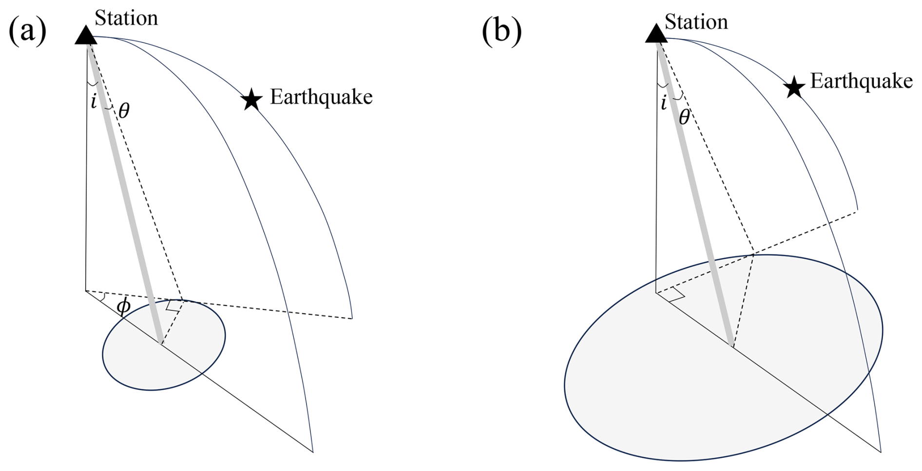
Figure 3 Relationship between the threshold angle and the deviation angle: (a) when the threshold angle is less than the wave incident angle, and (b) when the threshold angle exceeds it. In both cases, the gray line denotes the trajectory of the inter-station ray path, whereas the shaded region illustrates the area encompassed within the stable angular range.

In contrast, when θ₀>i (i.e., Γ>1), even coda waves radiated from earthquakes in a plane perpendicular to the inter-station plane fall within the stable angular range defined by θ₀ (see Fig. 3b). In this regime, a larger Γ implies a smaller i relative to θ₀, indicating that the late coda waves radiated in these deviated planes align more closely with the target inter-station ray path. Consequently, for a given core phase, a larger Γ value leads to a tighter convergence of correlation signals across different deviation planes within the selected time window.

Core phases retrieved from late coda correlations are characterized by steep incidence angles, which typically yield relatively large values of Γ. To illustrate this effect, we compare two representative core phases at an inter-station distance of 10.0°:

ScS wave. Travel time ≈1000 s, threshold angle θ₀≈18.0°, and incidence angle i≈3.0°, yielding Γ≈6.0.

PKIKP² wave. Travel time ≈2500 s, threshold angle θ₀≈11.0°, and incidence angle i≈1.0°, yielding Γ≈11.0.

The significantly higher Γ value for PKIKP² indicates that its reconstructed waveform exhibits greater convergence across diverse deviation planes compared to the ScS phase. This comparison demonstrates that for phases with steep incidence angles, contributions from earthquakes at all deviation angles must be accounted for. In such cases, even sources located far from the great-circle path can contribute constructively to the correlation signal, facilitating the robust reconstruction of deep-earth phases.

Figure 4 The computations of the CCF under three truncation angles.

3 Numerical Simulations

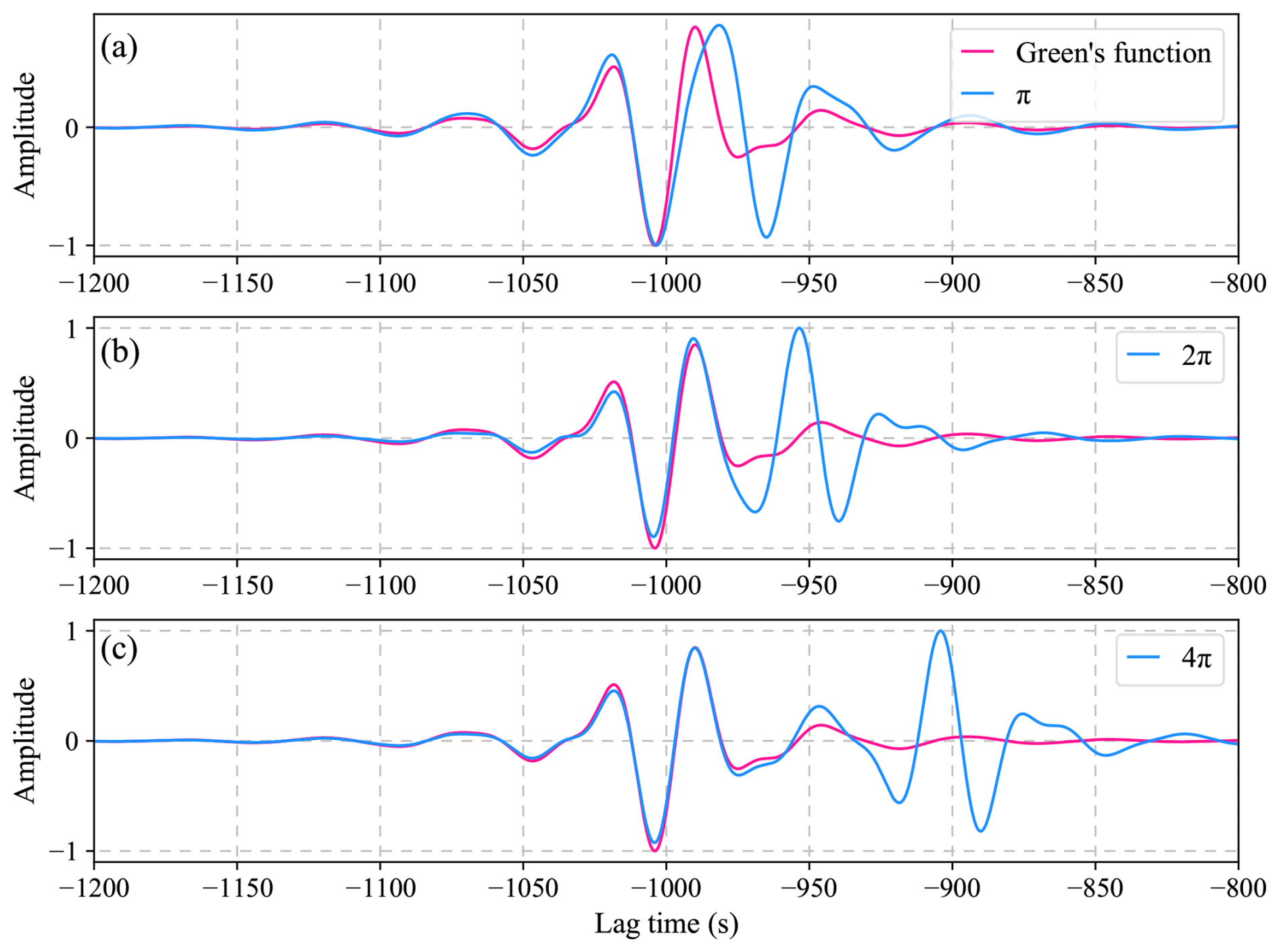
We perform a numerical computation to investigate the impact of wave correlation under locally uniform illumination. In the computation, we set the travel time of the reflected wave to 1000 s and wave correlation in the period range of 20–50 s. Then, we obtain the threshold angle θ₀=18° as in Eq. (20), corresponding to a 2π phase shift relative to the reflected wave. We also compute truncation angles for π and 4π phase shifts, obtaining θ₀=13° and θ₀=26°, respectively. These truncation angles are used as upper bounds in the integral of Eq. (10). For comparison, we compute the accurate arrival of the reflected wave using an upper bound of 180°. The results show: Within a π phase shift, the reconstructed reflected wave and truncation-induced spurious wave interfere, causing phase deviation in the reconstructed reflected wave. Within a 2π phase shift, the two waves align, allowing accurate recovery of the reflected wave's travel time. Within a 4π phase shift, the waves diverge, and the reconstructed reflected wave remains unaffected by integration truncation (Fig. 4). This supports the rationality of our non-interference criterion that uses a 2π phase shift to determine the threshold angle.

Given the small threshold angle in our simulation, we further examine correlation under a non-cosine travel-time difference distribution by setting the disturbance term in Eq. (13) as

$$\begin{array}{}\text{(24)}& \mathit{\delta }(\mathit{\theta },p)=-\mathrm{50}\mathit{\theta }{\sin }^{\mathrm{2}}\left(\mathrm{4}\mathit{\theta }\right).\end{array}$$

This function and its first derivative satisfy the constraints in Eq. (14). Integrating over θ from 0 to π and comparing the reconstructed wave with that from a cosine travel-time difference distribution, we find nearly identical phase information (Fig. 5). This demonstrates high reconstruction accuracy for travel times even under non-cosine travel-time difference distributions.

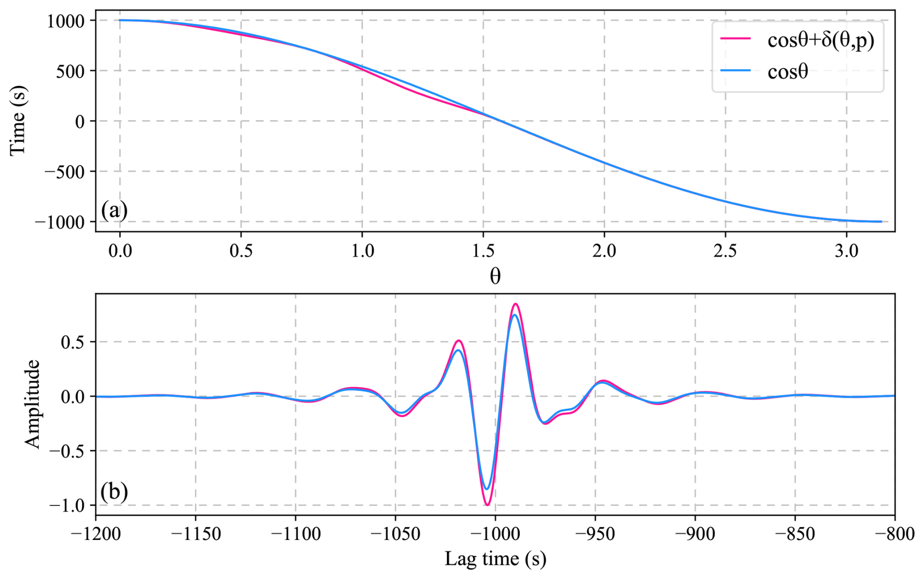
Figure 5 The computation of the CCF under a non-cosine distribution of travel time differences. (a) The travel time difference function; (b) The simulated CCF.

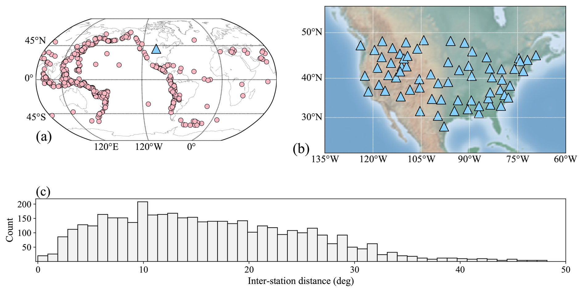
Figure 6 (a) Distribution of the large earthquakes (circles) and stations (triangles) used in this study, (b) enlarged view of the station distribution, and (c) histogram showing the number of inter-station distances in each stacking bin.

4 The Real-Data Test

We selected 205 large earthquakes (M≥6.8) from 2010 to 2020 with global distribution. For each event, we downloaded broadband waveforms from stations in the USArray Transportable Array. The spatial distribution of the earthquakes and stations is shown in Figs. 6a and 6b. For the late coda radiated by each earthquake, instrument responses were removed, and the data were bandpass filtered between 0.02 and 0.07 Hz (15–50 s period) to retain core-sensitive body wave energy. For each earthquake–station pair, we extracted the late coda time window from 10 000 to 40 000 s after the origin time. This window contains dominant multiply scattered waves that have sampled deep Earth structures. For each station pair and each earthquake, we computed the cross-correlation of the coda waveforms following the procedure of Bensen et al. (2007). We then calculated the deviation angle ϕ between the earthquake–station plane and the two-station plane. Correlograms were stacked within selected ϕ ranges and inter-station distance bins (bin width 1°). Arrival times of target phases were picked from the stacked correlograms using automated peak detection with manual verification. The number of cross-correlation functions stacked in each bin is statistically summarized in Fig. 6c.

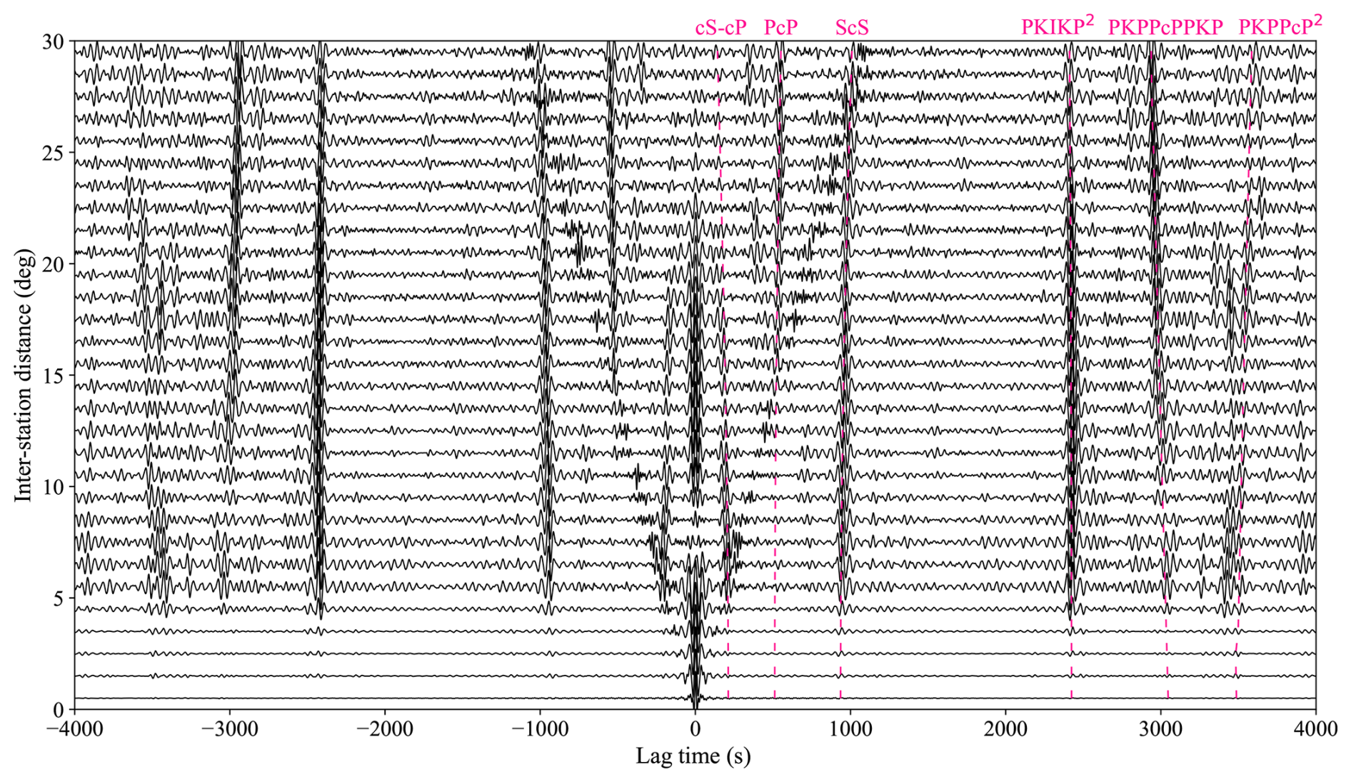
Figure 7 The stacked correlograms are shown, with selected prominent phases labeled. Dashed lines indicate the predicted travel times of the core phases, computed using the Taup toolkit with the ak135 reference model.

In the stacked correlograms, prominent deep Earth phases – specifically PcP, ScS, and PKIKP² – are clearly distinguishable (Fig. 7). To quantitatively evaluate whether the illumination condition has been satisfied, we performed a bootstrap analysis by progressively increasing the number of earthquakes in the stack from 10 to 120, in increments of 10. The stabilization of travel times with an increasing event count serves as a diagnostic for meeting the illumination condition. For each subset size, we performed 250 random realizations to compute the mean travel time and standard deviation for the extracted ScS and PKIKP² phases.

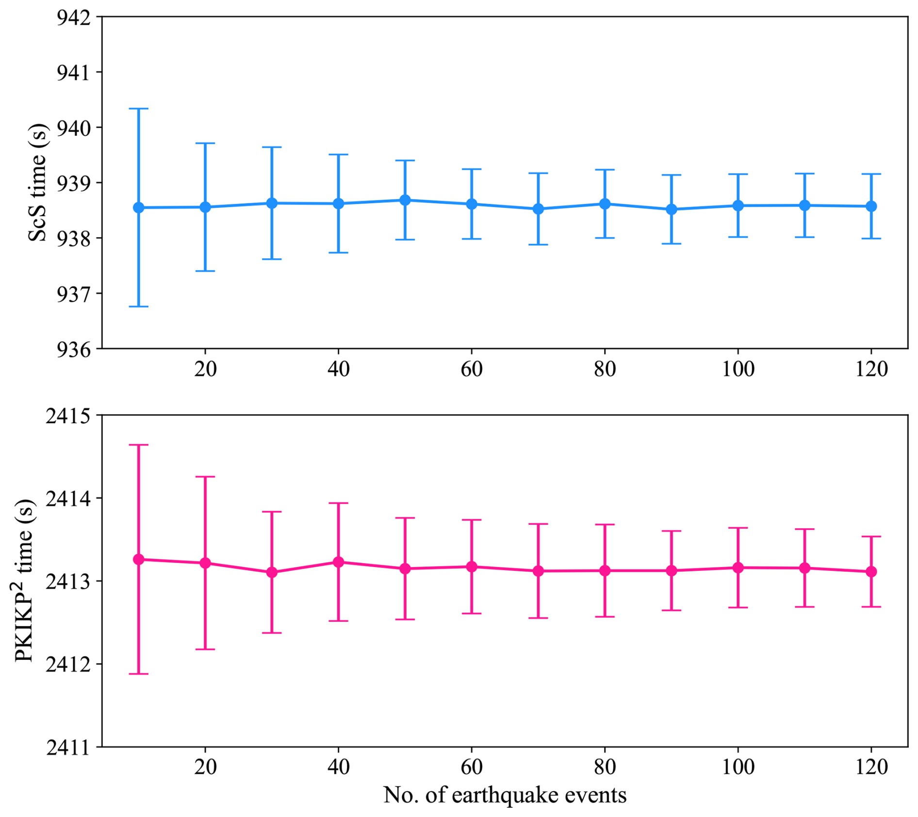
Figure 8 Statistics of the mean and standard deviation of wave travel times as a function of the number of earthquakes included in the stack.

Our results reveal two key findings (Fig. 8). First, for both phases, the mean travel time stabilizes and the standard deviation decreases as the number of earthquakes increases, indicating clear convergence toward a stable value. Second, significant travel-time deviations–exceeding ±1 s – are observed when fewer than approximately 20 earthquakes are used, particularly for the ScS phase. This indicates that a minimum event count is required to achieve locally uniform illumination. However, we emphasize that this threshold is not solely dependent on the event count, but also on the azimuthal distribution of sources, their focal mechanisms and the number of correlation traces stacked per distance bin. The cubic scaling relationship derived in Eq. (18) assumes locally uniform illumination; when this condition is violated – as seen in the smaller earthquake subsets – the scaling relationship breaks down, resulting in the observed high standard deviations.

According to our theoretical framework, when the locally uniform illumination condition is satisfied and the Γ value is large (as it is for both ScS and PKIKP²), correlation signals across different deviation planes should converge toward the true inter-station arrival time. To verify this convergence, we partitioned the correlograms based on specific ranges of the deviation angle ϕ. The resulting stacked correlograms exhibit clear signals in both the ScS and PKIKP² time windows; however, as predicted, the PKIKP² signals appear more focused than those of ScS (Fig. 9). This trend is further illustrated by comparing the azimuthal deviation (ϕ) ranges of (0, 20°) and (40, 60°) (Fig. 10a, b): while travel-time deviations for ScS reach up to 3 s, they remain nearly identical for PKIKP² (Fig. 10c, d).

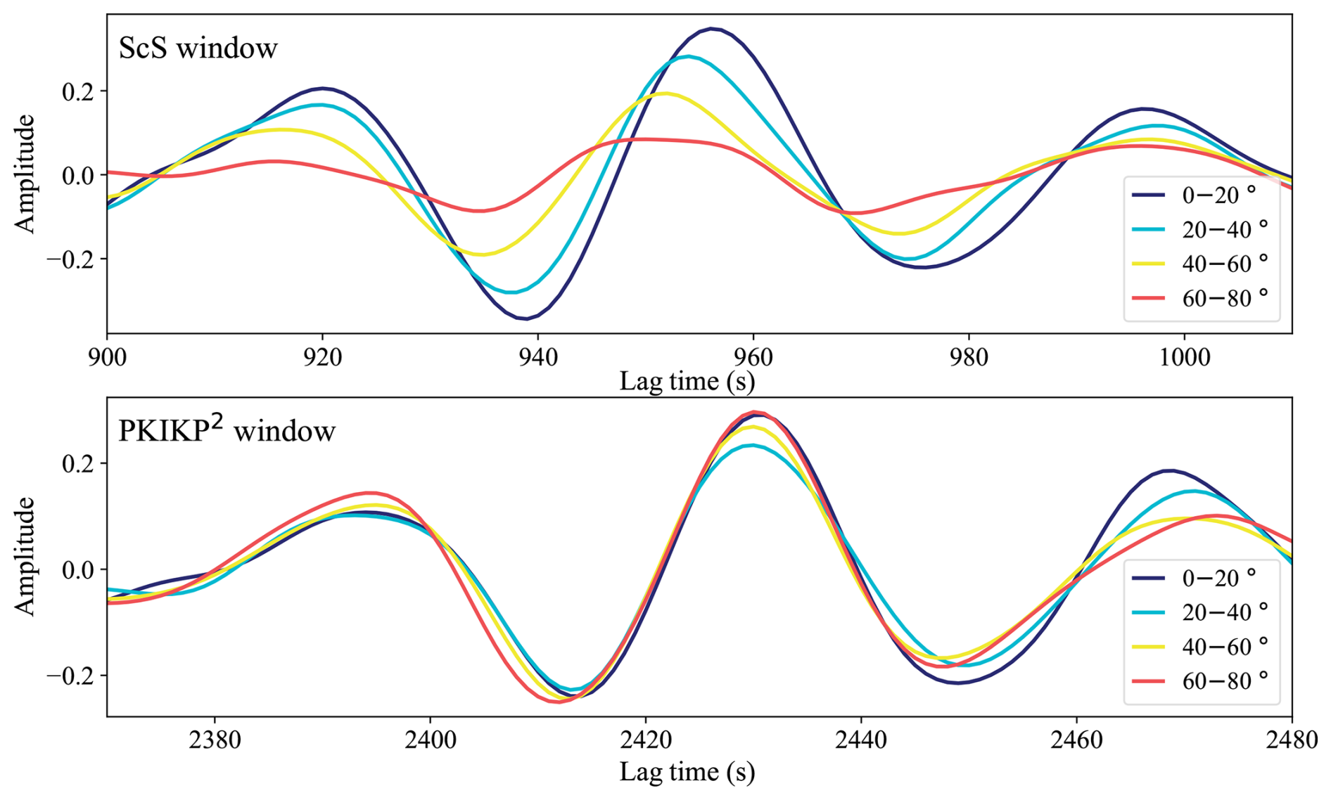
Figure 9 Variation in travel times of ScS and PKIKP²-like waves as a function of deviation angle range. The bin width for inter-station distance is 10°.

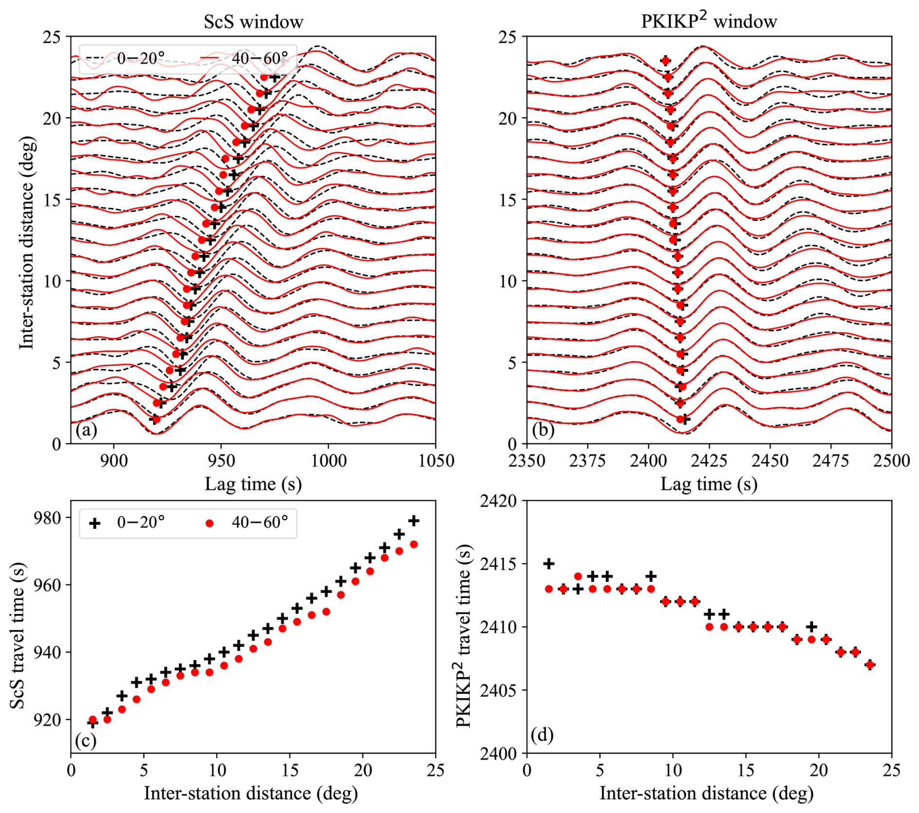
Figure 10 Comparison of (a) ScS and (b) PKIKP² time windows using earthquakes with ϕ in the ranges (0, 20°) and (40, 60°). (c) and (d) show the corresponding trough arrival times for ScS and PKIKP² across the two ϕ ranges, respectively.

5 Discussion

This study investigates the reconstruction of inter-station waves under conditions where the incidence of seismic waves is locally uniform along the propagation path. A critical angular threshold θ₀, defined in Eq. (12) as the ratio of the seismic wave period to the inter-station travel time, quantifies the extent of this locally uniform illumination. Equation (19) further demonstrates that the accuracy of travel time reconstruction scales with the cube of this threshold angle. This cubic scaling relationship reveals that even under ideal uniform illumination, small travel-time deviations persist – a finding consistent with surface wave dispersion studies in inhomogeneous media (Tsai, 2009). The relationship provides a practical criterion for assessing expected travel-time errors in reconstructed body waves based on readily available parameters: wave period and inter-station travel time.

Core phases are characterized by inherently small threshold angles due to their long travel times (e.g., θ₀≈11° for PKIKP² at 10° distance). This property has two important practical implications. First, high-precision travel-time extraction can be achieved under the locally uniform illumination condition according to Eq. (19). Second, late codas radiated from a modest number of sparsely distributed earthquakes may satisfy this condition – as demonstrated by our bootstrap analysis showing convergence with approximately 50–100 events (Fig. 8). Consequently, our approach relaxes the stringent requirements of traditional seismic interferometry, making it more applicable to practical coda correlation studies where global earthquake distributions are inherently non-uniform.

In Fig. 7, the reconstructed core phases at near-zero inter-station distances (<4°) exhibit systematically lower signal-to-noise ratios (SNR) than at larger distances. This pattern can be explained within our theoretical framework. The constructive interference required to build a specific phase (e.g., PKIKP²) depends on coda waves with incidence angles nearly identical to that of the target phase. For late coda waves with near-vertical incidence, the propagation path from the earthquake source to the station is substantially longer, resulting in stronger geometric attenuation and thereby reducing the amount of correlated late coda energy available for constructive interference. In addition, as shown in Fig. 6c, the number of correlation traces stacked in near-zero distance bins is relatively low compared to bins at moderate distances. The reduced stacking fold further limits the enhancement of coherent signals.

The near-vertical incidence of PKIKP² results in a high Γ value, which in turn facilitates an extremely tight convergence of correlation signals across different deviation planes (Figs. 9 and 10). This geometric advantage ensures that arrival times remain nearly identical regardless of the source deviation angle ϕ. A long-standing debate in coda correlation seismology centers on whether extracted phases represent true inter-station PKIKP² arrivals (the Green's function) or a modified wavefield (I2*) whose travel times exhibit a systematic dependence on source distribution (Wang and Tkalčić, 2020b, a; Costa de Lima et al., 2022). Based on our theoretical analysis and empirical results, we propose that the transition from a biased I2* measurement to a true PKIKP² phase travel time occurs when the following two conditions are jointly satisfied:

1. Illumination condition for stable reconstruction: The angular range of incident waves meets or exceeds the phase-specific critical angle θ₀, ensuring that the stationary phase zone is adequately sampled. This condition depends on the number of earthquakes, focal mechanisms, their azimuthal distribution relative to the inter-station path, and the distribution of inter-station directions stacked per distance bin. The degree to which this condition is satisfied can be evaluated quantitatively through bootstrap convergence analysis (Fig. 8), where stabilization of travel times with increasing event count indicates that the illumination condition has been achieved. It can also be assessed by examining the convergence of the correlation signals across different deviation planes.

2. Smoothness condition for accurate travel time recovery: The structural setting along the ray path must yield a sufficiently smooth deviation function δ(θ,p), rendering higher-order terms in Eq. (19) negligible. Seismic ray theory assumes a smooth velocity structure (Chapman, 2004), which produces a smooth wavefront and thus smooth travel time variations from the source to the receiver and its surroundings – which in turn ensures a smooth δ(θ,p). Our analysis therefore remains valid within the ray-theoretical framework. Although this smoothness condition cannot yet be independently verified in the real Earth, it is a necessary prerequisite for interpreting stable measurements as true arrivals, pending future validation against earthquake-derived empirical travel times.

This unified interpretation suggests that the I2* phenomenon and true PKIKP² phase reconstruction are not mutually exclusive, but rather endpoints on a continuum defined by the degree to which locally uniform illumination and structural smoothness are achieved. In previous studies where the I2* effect was dominant, the illumination condition was likely not satisfied due to limited event counts or restricted azimuthal coverage – a scenario mirrored in our bootstrap results when using fewer than 20 earthquakes (Fig. 8). In contrast, the stable PKIKP² travel times reported here, achieved using a globally distributed dataset spanning a decade, satisfy these criteria. Consequently, our theoretical framework reconciles these seemingly contradictory findings by providing a generalized criterion for the extraction of true travel times from the late coda.

6 Conclusions

This study presents a perturbation analysis to evaluate the accuracy of travel-time reconstruction for core phases derived from late earthquake coda correlations under conditions of locally uniform wave incidence along the core-phase propagation path. We introduce a dimensionless parameter, defined as the ratio of seismic wave period to inter-station travel time, to quantify the critical angular threshold for effective reconstruction. Perturbation analysis reveals that the travel time accuracy scales with the cube of this threshold, indicating that localized uniform incidence ensures high-precision reconstruction of core phases, which are inherently characterized by low threshold values. Numerical simulations and empirical coda correlation tests sustain our theoretical findings. Our results demonstrate that accurate travel times of inter-station core phases can be reliably extracted using late coda waves from a sufficiently large number of earthquakes distributed across all deviation angles. This approach provides a practical and robust foundation for coda correlation studies, enhancing confidence in using reconstructed core phases as true empirical arrivals for interferometric imaging of Earth's deep interior.